1. Introduction
Debris flows, which are highly concentrated mixtures of water, soil, and debris can cause devastating damage as they propagate downslope, making their mitigation and control a necessary concern (Hungr et al., 2005, Han et al., 2015). In natural environments, debris flows rarely propagate on a flat, uninterrupted trajectory. Instead, they encounter complex and uneven terrain characterized by various obstacles and irregular topography. These irregularities can take the form of bottom roughness, topographic features such as humps and hilly terrains, or even man-made structures like check dams, groundsills, or other mitigation measures (Iverson, 1997). One of the established techniques for mitigating debris flows involves the strategic placement of groundsills, which are structural barriers designed to dissipate energy, trap sediment, and regulate flow propagation (Choi et al., 2018; Ng et al., 2014). When debris flows interact with bottom irregularities or man-made structures, the changes in topography introduce additional drag forces that decelerate the flow velocity. The presence of obstacles and uneven surfaces disrupt the continuous flow, causing a deceleration in the progression of the debris flow (Jacob et al., 2005). Consequently, the flow dynamics become inherently unpredictable and complex, as the flow dynamics are influenced by the interactions between the debris material and the varying bottom irregularities (Sand-Jensen, 1998). Moreover, the presence of larger solid particles in the mixtures may interact differently with the obstacles, which can significantly influence the sediment trapping between them (Han et al., 2024).
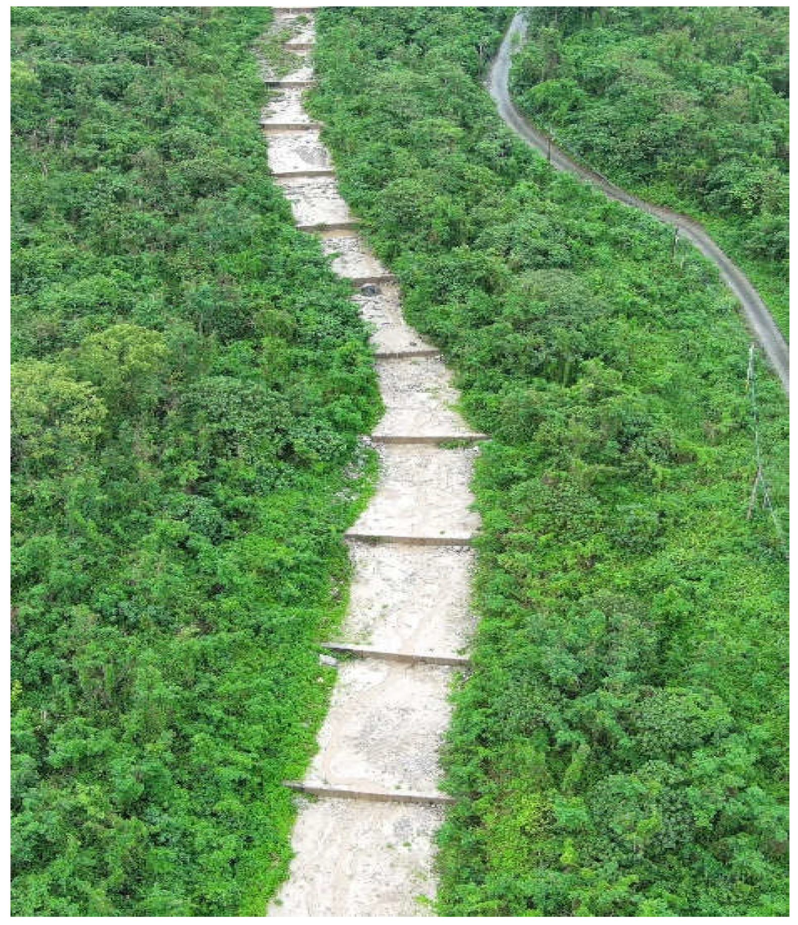
Recently, several researchers investigated gravity currents over a smooth rigid boundary moving down the slope (Britter and Linden, 1980), flow over or through obstacles (Hatcher et al., 2000), and flow over permeable surfaces (Marino and Thomas, 2002). To better understand how surface roughness affects fluid flow, experimental and theoretical studies have been conducted on various artificial roughness elements, leading to the classification of different ’types’ of roughness with effects comparable to those observed in natural environments (Rouse, 1965). One such approach is to use beam-type groundsill arrays, which are transverse structures installed on river channels to guide the flow, reducing velocity, mitigating erosion, and adjusting bed slope (Shima et al., 2016; Lin et al., 2024; Ikhsan et al., 2009). Ground sills are engineered structures designed to reduce the sediment-laden flow velocities and increase sediment deposition upstream while allowing flow to propagate over them (Lin et al., 2008). However, the practical implementation of ground-sills has revealed challenges in both design and operation, where the intended functionality often differs from the observations in the real field (Lin et al., 2008). For instance, studies have demonstrated that ground sills enhance sediment deposition upstream and stabilize channel morphology, but real-world performance has varied depending on the design and context. Addressing the complexity of ground-sill projects requires a more integrated strategy rather than fragmented solutions (Bagli, 2019). In Taiwan, debris flows frequently occur due to the mountainous terrain, heavy rainfall, and frequent typhoons (Jan and Chen, 2005). This has necessitated the implementation of various mitigation measures, including check dams, slit dams, and groundsills (Jan and Chen, 2005). After the 1990 debris-flow event, a series of check dams were constructed along a debris-flow gully in Hualien County to manage debris transport and reduce damage (
Figure 1). These structures function similarly to beam-type groundsill arrays, which are transverse structures installed on river channels to guide the flow, reduce velocity, mitigate erosion, and adjust bed slope.
Research on flow over groundsills has mainly focused on Newtonian fluids, especially regarding erosion control and riverbed stabilization (Hairani and Legono, 2016). Recently, however, interest has grown in non-Newtonian fluids due to their complex flow characteristics and practical applications (Bigham, 2020). Observing non-Newtonian flow behavior experimentally is challenging because of their intricate rheological properties and flow dynamics. Consequently, we employed numerical simulation in this study to investigate the flow behavior of debris flow approximated by the Bingham Fluid Model with two rheological parameters, namely the Bingham yield stress () and viscosity (). Debris flows can be typically classified into three main categories: mudflows, which consist primarily of fine materials such as clay and silt (Blasio, 2011), and stone- or boulder-rich debris flows dominated by larger particles (Julien & O’Brien, 1997). Between these two extremes, intermediate debris flows exist with varying sediment compositions and concentrations (Iverson and Denlinger, 1987). This study simulates the propagation of sediment mixtures modeled as the debris flows that follow the Bingham Fluid Model, as they move over a beam-type array of groundsills positioned within an inclined channel set at a 15° slope. The groundsill array density refers to the spacing between consecutive groundsills, represented by the ratio between the spacing and their relative height (i.e., ). It is classified as high array density () and low array density (). Our main goal is to investigate how varying this groundsill array density influences the flow behavior of sediment mixtures including flow depth, front position of the flow, and flow velocity.
2. Materials and Methods
2.1. Sediment Mixture Preparation
The sediment mixtures are highly concentrated clay-silt-water mixtures having a sediment fraction
. A volume,
of sediment was well mixed with tap water of volume,
to form a sediment mixture with a sediment fraction,
, as shown in Eq. 1.
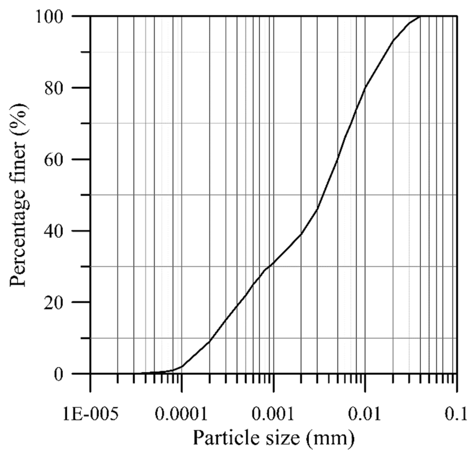
The clay-silt materials were used as the sediment in the present experiments, which were collected from a reservoir sediment deposition. After washing them multiple times to remove any organic debris, the materials were oven-dried and stockpiled for experiments. As shown in
Figure 2, the particle size distribution of the clay-silt materials yielded a medium diameter (
) of 0.0036 mm and a particle density of 2.65 g/cm
3. The sediment mixtures prepared for this study had a sediment fraction
.
2.2. Rheometer Setup and Measurement of Rheological Parameters
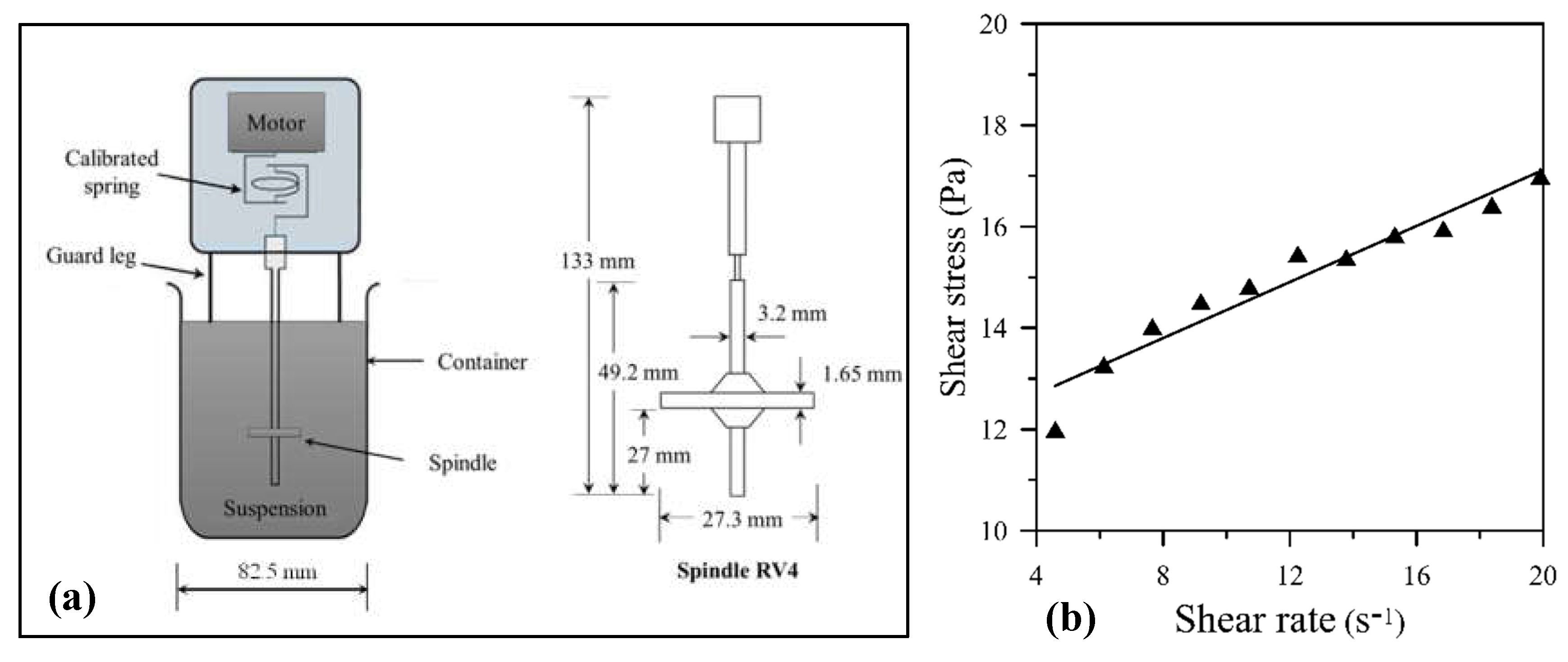
To characterize the rheological properties of the sediment mixtures, a conventional Brookfield rheometer (model DV-III) was utilized. This rheometer operates by rotating a spindle (RV-6) within the sediment mixture and measuring the torque required to overcome the viscous resistance during the spindle’s rotational motion. The spindle is immersed into the mixture contained in a 600 ml glass beaker, and the rheometer is controlled by a computer running the Rheocal-32 software. A schematic representation of the rheometer test, depicted in
Figure 3a, follows the same approach we used in our previous studies (Jan and Dey, 2022; Dey et al., 2021).
The measurements were conducted in a controlled shear rate mode, where the rotational speed of the spindle was regulated, and the corresponding torque required was recorded. To ensure the repeatability and reliability of the results, each test was performed at least three times, and the final reported values are the average of these repeated measurements. These measurements were carried out at room temperature, approximately 25°C. The recorded spindle speed and torque values were then converted to shear rate and shear stress, respectively, using Mitschka’s method (Mitschka, 1982), as described by Dey et al. (2021). Subsequently, the calculated shear stress and shear rate data were used to characterize the rheological properties of the sediment mixture, as illustrated in
Figure 3b. The relationship between shear stress and shear rate follows the Bingham Fluid Model, which is expressed mathematically in Eq. 2.
in which
Bingham yield stress (Pa),
Bingham viscosity (Pa.s), and
shear rate (1/s). The measured values of
and
for sediment mixture used in this study with
, were 12.83 Pa and 0.28 Pa.s, respectively. The rheological parameters (
and
) of these Bingham fluids are functions of sediment fraction (
) and sediment size (
), expressed as
. The parameter
represents the influence of larger particles within the mixture by changing its rheological parameters (Major and Pierson, 1992; Dey et al., 2021; Jan and Dey, 2022).
At low shear rates (), shear stress of sediment mixtures used in this study first increases and then decreases, potentially causing data scatter (Dey et al., 2021; Ancey and Jorrot, 2001). In contrast, at higher shear rates (), the shear stress-shear rate relationship aligns well with the Bingham fluid model. The Bingham fluid model is widely used in numerical simulations of debris flow movement not only for its simplicity but most of the natural debris flows exhibit a shear rate within the range of 5 to 20 s⁻1 (Major and Pierson 1992; Jan et al., 2019; Dey et al., 2021). Therefore, we focus on the rheological properties of sediment mixtures tested in this study within the shear rate range of s⁻1.
3. Numerical Simulation Methodology
In this study, we utilized the commercial CFD software Flow-3D to simulate the flow behavior and dynamics of sediment mixtures flowing over a beam-type array of groundsills placed in an inclined channel. The simulation employs the principles of mass conservation (the continuity equation) and momentum conservation (Navier-Stokes momentum equation) to comprehensively characterize the complex dynamics of three-dimensional fluid movement. The fluid phase interface is specified through the utilization of the Volume-of-Fluid (VOF) method, which accurately monitors the interface between different fluids or between a fluid and a solid. The Flow-3D User Manual provides detailed descriptions and mathematical formulations of the mass continuity and momentum equations governing the fluid flow dynamics (Flow Science, 2008).
In this study, the Flow-3D solver uses the Navier-Stokes equations combined with the Volume of Fluid (VOF) method to simulate sediment mixture flow on an inclined channel. The Navier-Stokes equations incorporating the Bingham Fluid Model can be expressed as:
where
are the components of the velocity vector u,
is the time,
is the density of the mixture,
is the pressure,
is the stress tensor for the Bingham Fluid Model,
is the i-th component of the gravitational acceleration vector.
The stress tensor
for the Bingham Fluid Model is defined as:
where
is the Bingham yield stress,
is the Bingham viscosity,
are the components of the rate of strain tensor,
is the magnitude of the shear rate tensor. The above Eqs. (
) modeled the sediment mixtures tested in this study as a single-phase Bingham fluid. When modeling debris flows as single-phase fluids, the effects of larger particles, such as pebbles and rocks, are typically captured through the density of the mixture (
), and rheological parameters (i.e., yield stress,
and viscosity,
). Although this approach simplifies the system, the single-phase assumption can still offer valuable insights into the large-scale behavior of debris flows (Uchida et al., 2019; Lin et al., 2022).
3.1. Inclined Channel and Groundsill Array Setup
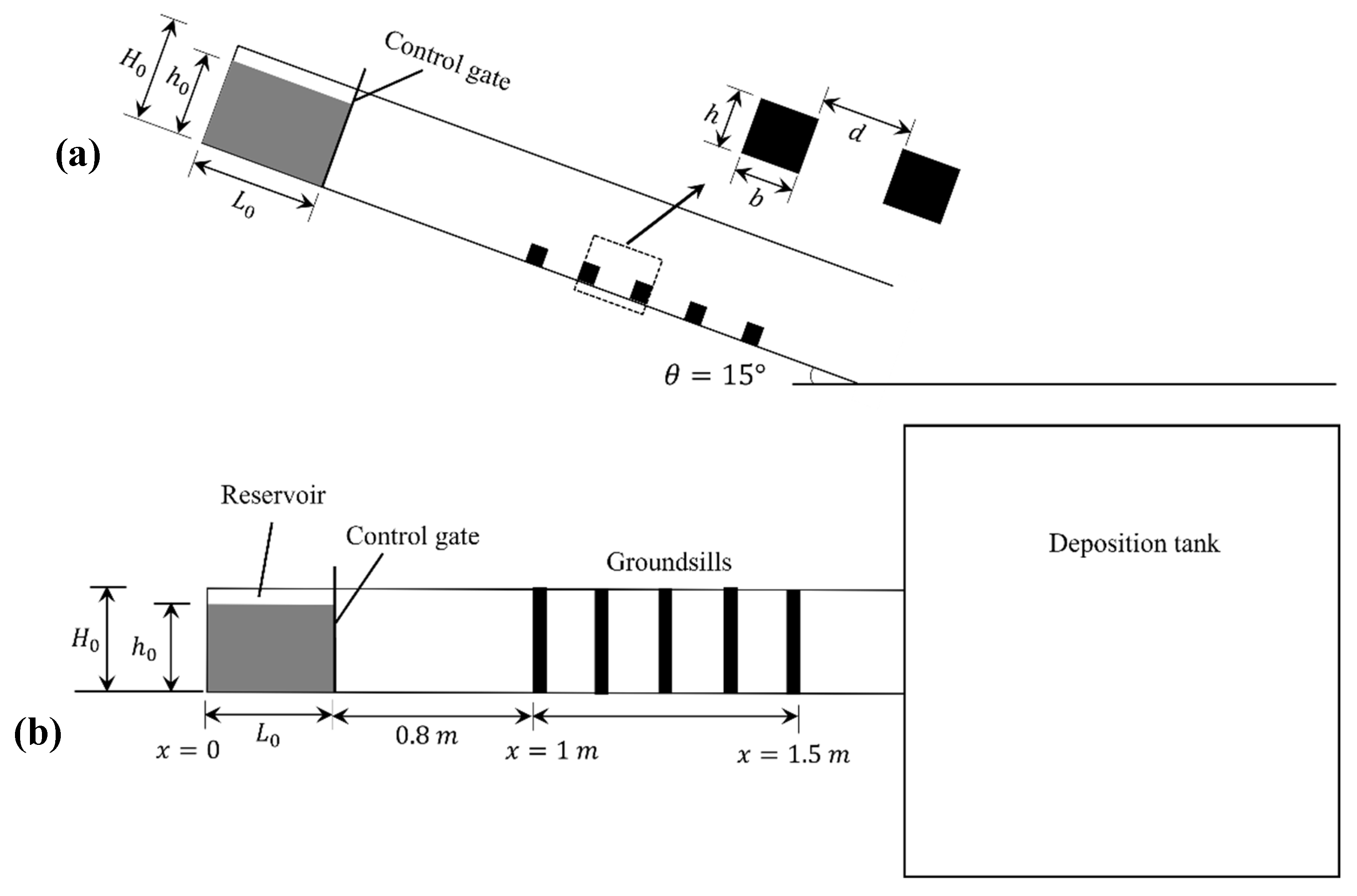
A laboratory-scale inclined channel was designed using AutoCAD software, with dimensions of 2.00 m length, 0.10 m width, and 0.1 m height. The channel bottom and walls were constructed from 5-mm-thick plexiglass material. At the upstream end of the channel, spanning
m in length and separated by a 5-mm-thick, 0.10-m-wide control gate to form a reservoir. The sediment mixtures used within the reservoir had a total volume of approximately 2 liters, characterized by dimensions
m and
m. The initial dimensions of the reservoir were characterized by length (
) and height (
), as shown in
Figure 4. The beam-type array of groundsills was placed along the inclined channel at a distance of 0.8 m from the control gate (
Figure 4b). This arrangement allowed the sediment mixtures to have sufficient flow length to develop before interacting with the groundsills.
.
The beam-type groundsills had initial dimensions of height (
), and length (
), as shown in
Figure 4a. Notably, the length of these groundsills aligned with the width of the channel (W = 0.1 m). All the groundsills were positioned over a length spanning 0.5 m in the middle of the inclined channel, which is within the range of
m as shown in
Figure 4b. This setup allowed us the investigate the flow behavior and dynamics of sediment mixtures as they interacted with the beam-type array of groundsills in the inclined channel. Field investigations have shown that the majority of debris flows occur in gullies with channel slopes ranging from 10° to 20° (Tsunetaka et al., 2019; Pierson, 2020). Therefore, in this study, a
channel slope was used to approximate the typical range observed in natural debris flows, ensuring the experimental results are relevant to real-world observations (Tsunetaka et al., 2019; Pierson, 2020). The design considerations, such as the channel dimensions, reservoir configuration, and groundsill placement, were carefully chosen to facilitate a comprehensive study of the fluid-sediment interactions and associated physical processes.
3.2. Groundsill Array Configuration
To simulate sediment flow over the array of groundsills, the beam-type groundsills were positioned at various array densities. The dimensions of the groundsill are illustrated in
Figure 4a, with respective values of
m for the base width and
m for the height. The array density is characterized by the ratio (
), where
is the spacing between two consecutive groundsills, and
is the height of the groundsill. In this study, five different array densities were simulated, with the (
) ratio ranging from 2 to 10 (
Table 1). Based on the density of the groundsills, the array density can be broadly categorized as low array density (
) and high array density (
), as illustrated in
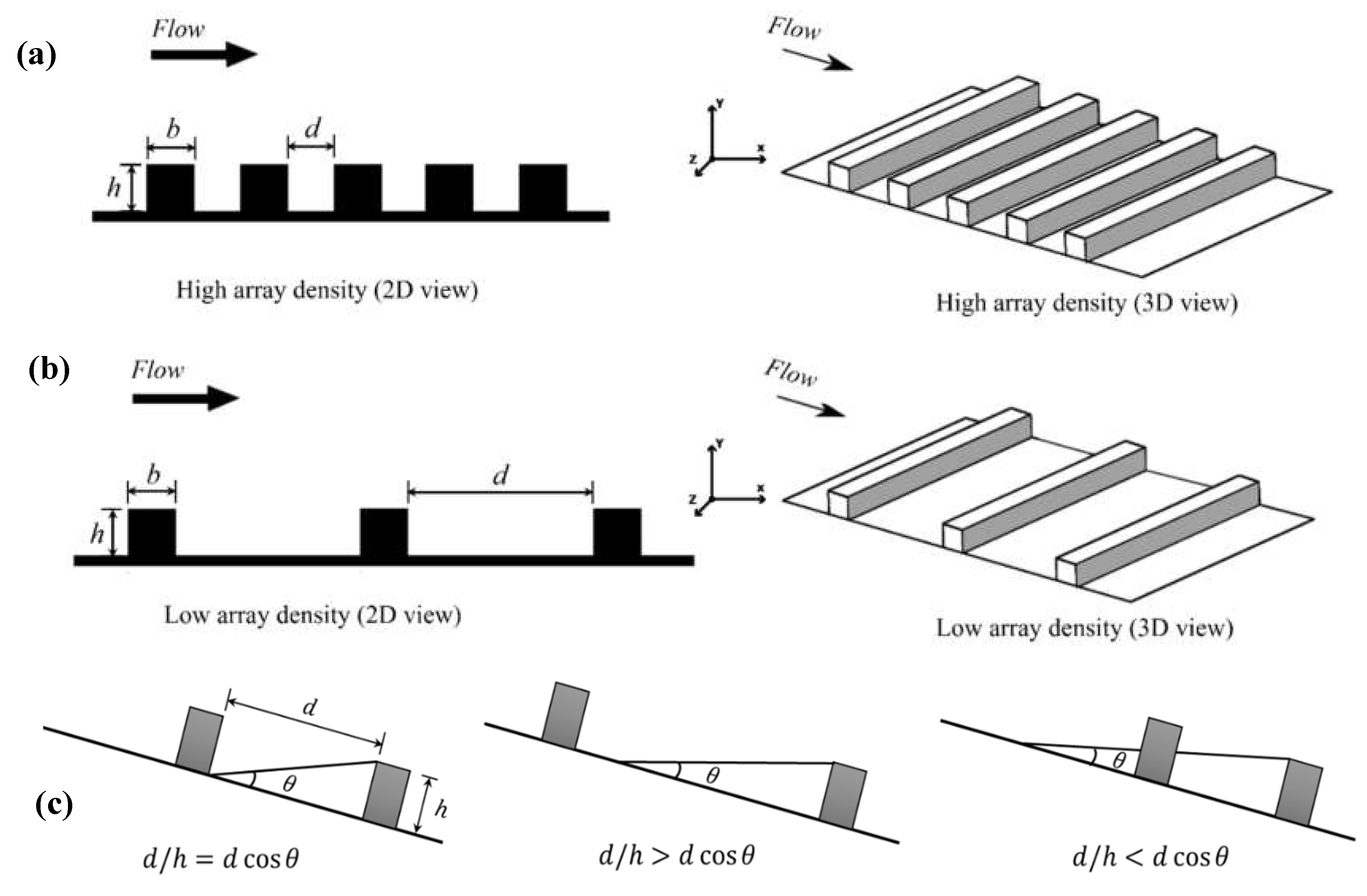
Figure 5. The categories of high and low array density can be defined based on the geometric relationships provided in Eqs. 5a and 5b:
For a channel slope of
, Eq. 5a defines a high array density with
less than
, and a low array density with
. High array densities have smaller spacings, which lead to different flow behaviors compared to low array densities with larger
values (Wu, 2022).
Figure 5c shows a schematic diagram for the definition of groundsill array density illustrating the relationship between
and channel slope,
.
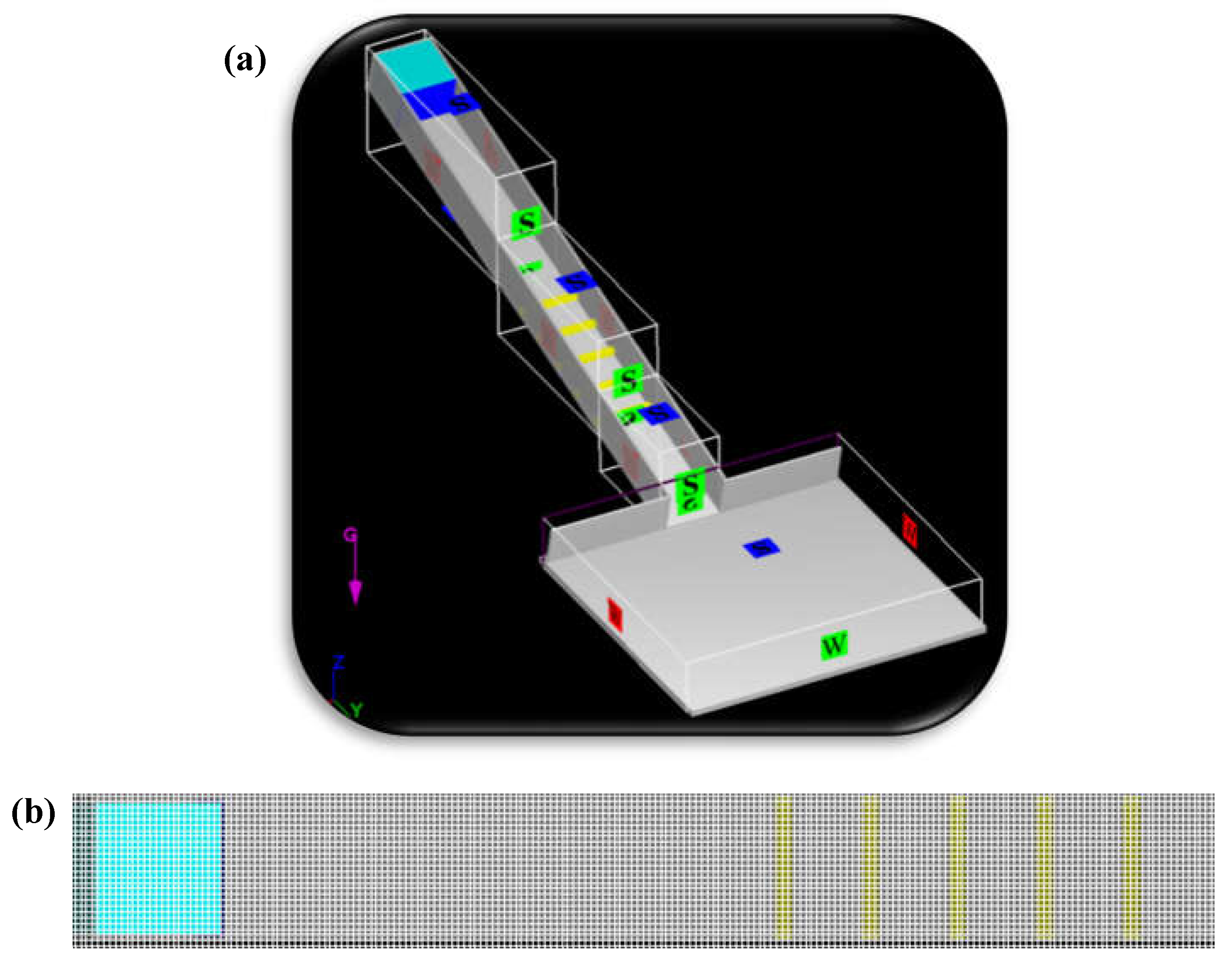
3.3. Simulation Domain, Boundary, and Initial Conditions
After creating the models in AutoCAD 3D, the channel geometry, reservoir column, and control gate were seamlessly integrated into the Flow-3D software for numerical simulation. The non-slip boundary condition is considered within the Flow-3D framework for the inclined channel with a rigid bed and wall configuration. At the inlet and outlet boundaries of the computed domain, a “wall (W)” boundary condition was applied to emulate a virtual barrier (
Figure 6a). This “wall” boundary condition was also extended to the bottom surface and lateral sides of the channel, creating a confined flow domain. Further, we applied a no-slip wall boundary condition on the bottom surface, which ensures that the flow velocity at the boundary is zero, thus simulating the frictional resistance imposed by the groundsill on the sediment mixtures. This boundary condition is integrated with the turbulence and sediment transport models within Flow-3D, allowing the frictional effects to be incorporated into the governing equations of the flow (Flow Science, 2008). To characterize the unobstructed free surface, the “symmetry (S)” condition was employed. This condition allows for the proper representation of the air-fluid interface and its dynamics. A geometry resolution of 0.002 mm was employed within the channel, gate, and fluid regions to better represent the boundaries of walls, bottom surfaces, and interfaces in the flow simulation (
Figure 6b). The lifting speed of the sliding gate was set at 0.3 m/s, which corresponds to the observed lifting speed during experimental investigations by Jan and Dey (2024).
4. Results and Discussions
4.1. Sediment Mixture Propagation
After the removal of the control gate, the sediment mixture starts to move from the reservoir, propagate downward, and interact with the groundsills. For high array density (specifically, ) the propagation of sediment mixtures is significantly impeded. A portion of the sediment mixtures are trapped and accumulate behind the groundsills. In contrast, for the low array density case (specifically, ), the sediment mixtures propagate more freely over the widely spaced groundsills. With larger gaps between the groundsills, the sediment mixtures can flow with less obstruction and deposition compared to the high array density case.
4.2. Temporal Evolution of the Flow Front
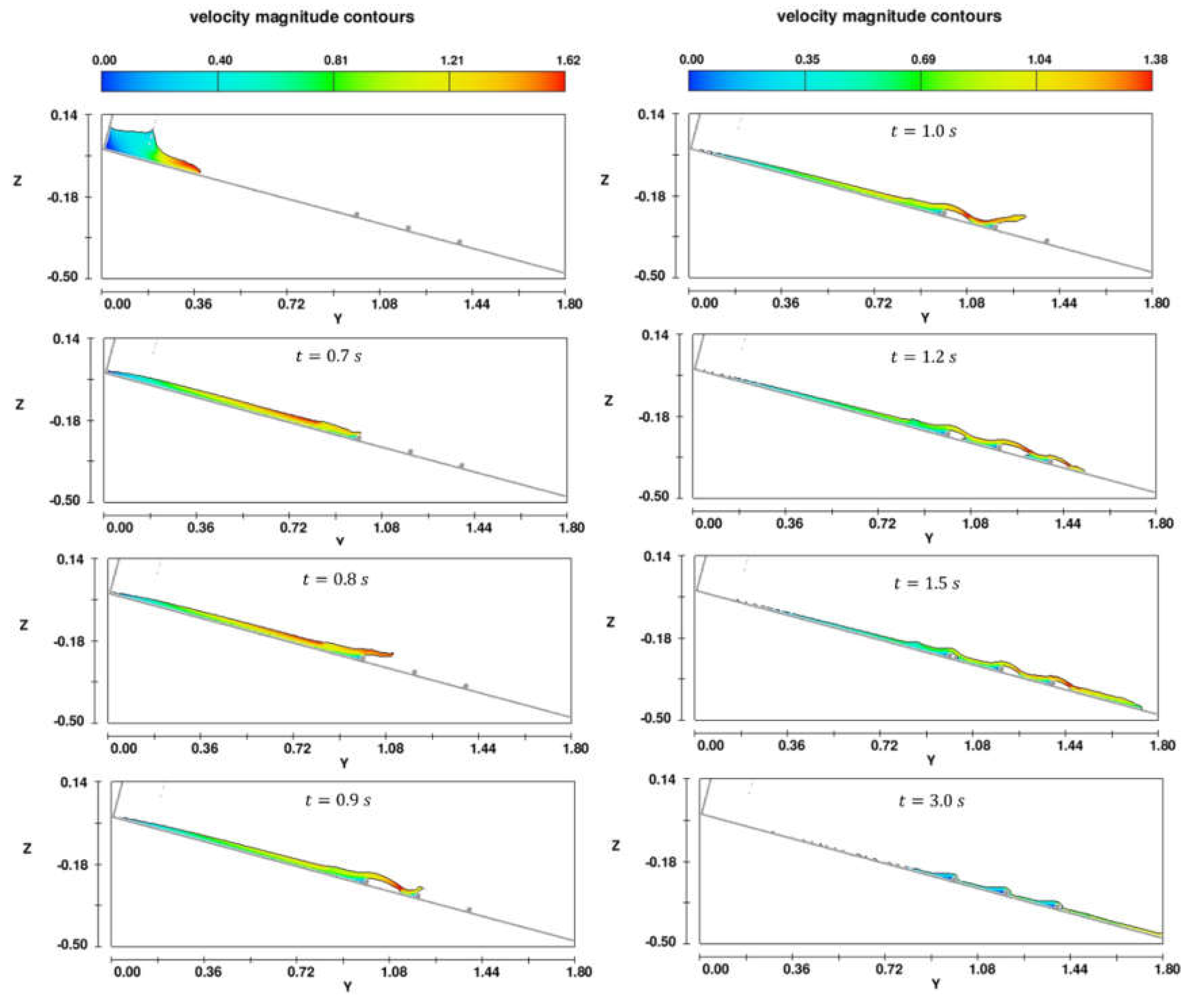
Figure 7 shows the velocity magnitude of sediment mixtures propagating over a low array density of groundsills in the inclined channel at different time frames. At
, after releasing the sediment mixture from the reservoir, the velocity of the mixture is relatively high near the flow front. As time progresses to
, the sediment mixtures start interacting with the groundsills, obstructing the flow and slightly decreasing the velocity near the front. By
, as the mixtures propagate further over the groundsills, the velocity near the front continues decreasing due to the increased resistance. At
, the sediment mixtures have traveled even further, and the velocity near the front is lower. Finally, at
, after the sediment mixtures have propagated over the entire array of groundsills, the velocity near the front is very low (
Figure 7).
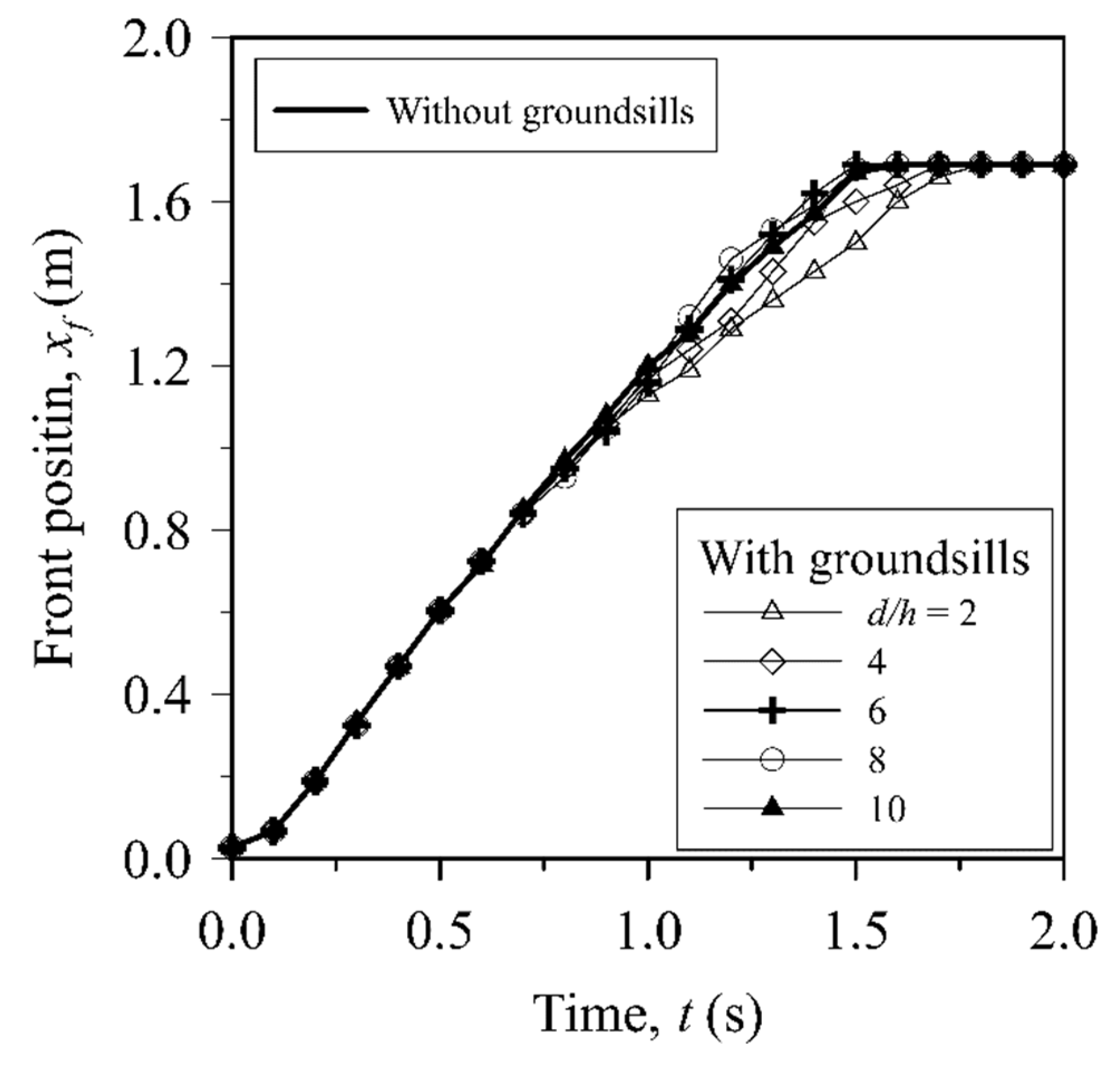
Figure 8 presents the evolution of the flow front position over time for sediment mixtures propagating with and without the presence of a groundsill array. The data points for involving groundsills demonstrate a slower propagation of the flow front compared to without groundsills. This observation indicates that the presence of groundsill obstructions impedes flow propagation and retards the propagation of the sediment mixture front. The influence of groundsill array density is evident in the flow front behavior. Higher groundsill array densities, characterized by smaller
ratios, lead to more obstructed flow conditions with reduced flow depths and slower front propagation. However, these high-density arrays also result in higher localized velocities due to the constrained flow paths. On the other hand, lower array densities, represented by larger
ratios, allow for smoother propagation with less obstruction but also lower overall velocities. Interestingly, it is observed that at times between
1.2 and 1.5 s, for lower array densities (
8 and 10), the flow front travels faster than the cases without groundsills (
Figure 8). This unusual behavior might be attributed to the increased local velocities induced by the spacing between groundsill arrays.
4.3. Influence of Groundsill Array Density on the Flow Profiles
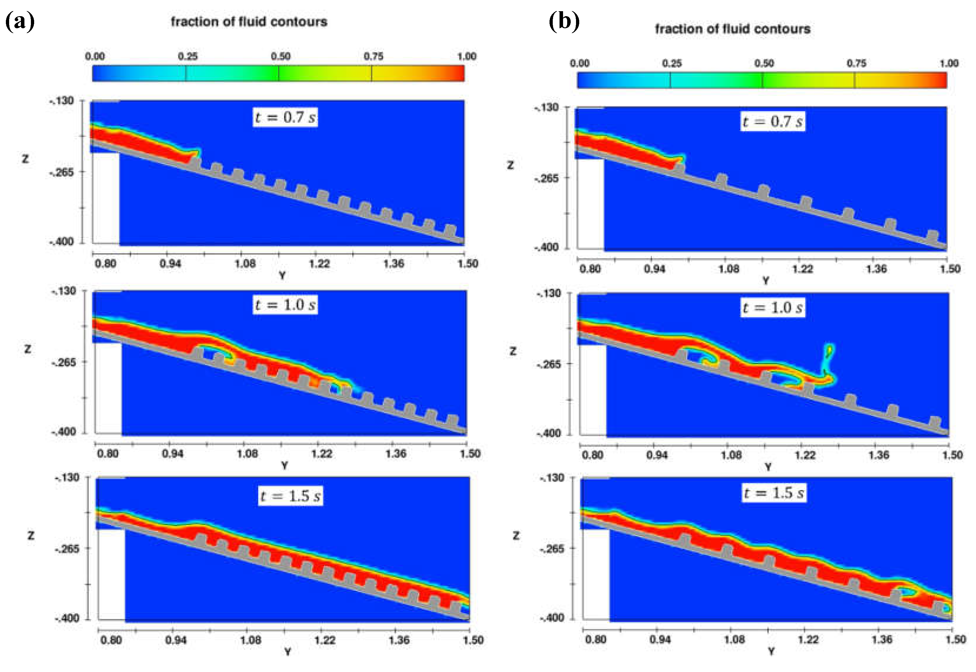
The contour plots in Figs. 9a-e presents the fraction of sediment mixture at three different simulation times: 0.7, 1.0, and 1.5 s for flow over groundsills at various array densities ranging from
to
. Based on these figures, we can observe how the flow patterns and extent of sediment mixture propagation vary with the groundsill array density. For high array densities (
2 and 4) at
, the sediment mixture flows relatively smoothly over the closely spaced groundsills with minimal disturbance (
Figure 9a and 9b). However, at later times (
and
), the mixture exhibits a more wavy pattern as it propagates over the groundsills, indicating increased interaction and disturbance caused by the groundsills. The sediment mixture also appears to propagate slightly less far downstream for
2 compared to
4, suggesting a stronger influence of the more closely-spaced groundsills on the flow.
For low array densities (
6, 8, 10), even at the early stage (
), the sediment mixture flow exhibits a more irregular pattern, with pockets of higher and lower fluid fractions forming around the widely-spaced groundsills (
Figure 9c-e). At later times (
and 1.5
s), the flow patterns become increasingly complex, with noticeable wavy structures and fluctuations in the fluid fraction distribution. It can be observed that as the
ratio increases, the flow patterns become more complex and disturbed, with more wavy structures and irregular fluid fraction distributions. Furthermore, the extent of sediment mixture propagation downstream reduces, indicating a stronger influence of the more closely spaced groundsills on the flow behavior.
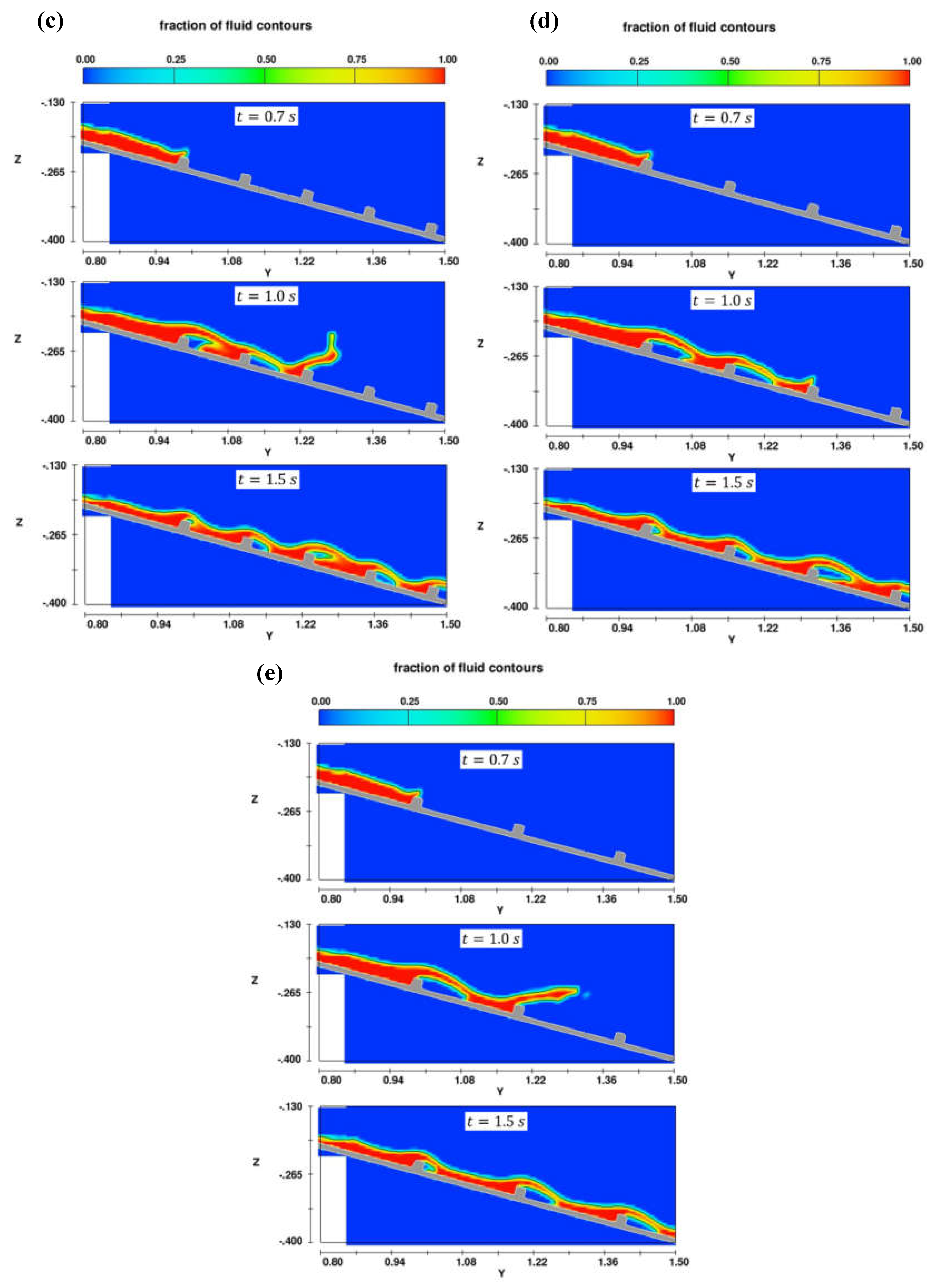
Figure 10 presents the sediment mixture fraction contours at a time
, displaying a snapshot of how the sediment deposits appear after overflowing the groundsills and settling. When
, the sediment mixture overflows the groundsills almost uniformly, with a significant portion of the mixture flowing over each sill. The fluid fraction contours reveal that the sediment is well-distributed across the array, with minimal accumulation between the sills, nearly filling the space between them (
Figure 10a). As the
ratio increases to 6, the overflow becomes less uniform, with visible gaps emerging between the areas of sediment overflow. The fluid fraction buildup between the sills roughly forms a triangular shape, with the highest deposit height near the base upstream of each groundsill, gradually tapering off further upstream (
Figure 10b). At
, the sediment mixture propagates over the groundsills with even larger spacing. The overflow becomes concentrated near the sills, with minimal sediment accumulation in the spaces between them (
Figure 10c). This indicates that at higher
ratios, the sediment mixture tends to bypass the intermediate areas (
Figure 9), resulting in sediment deposition primarily near the sills.
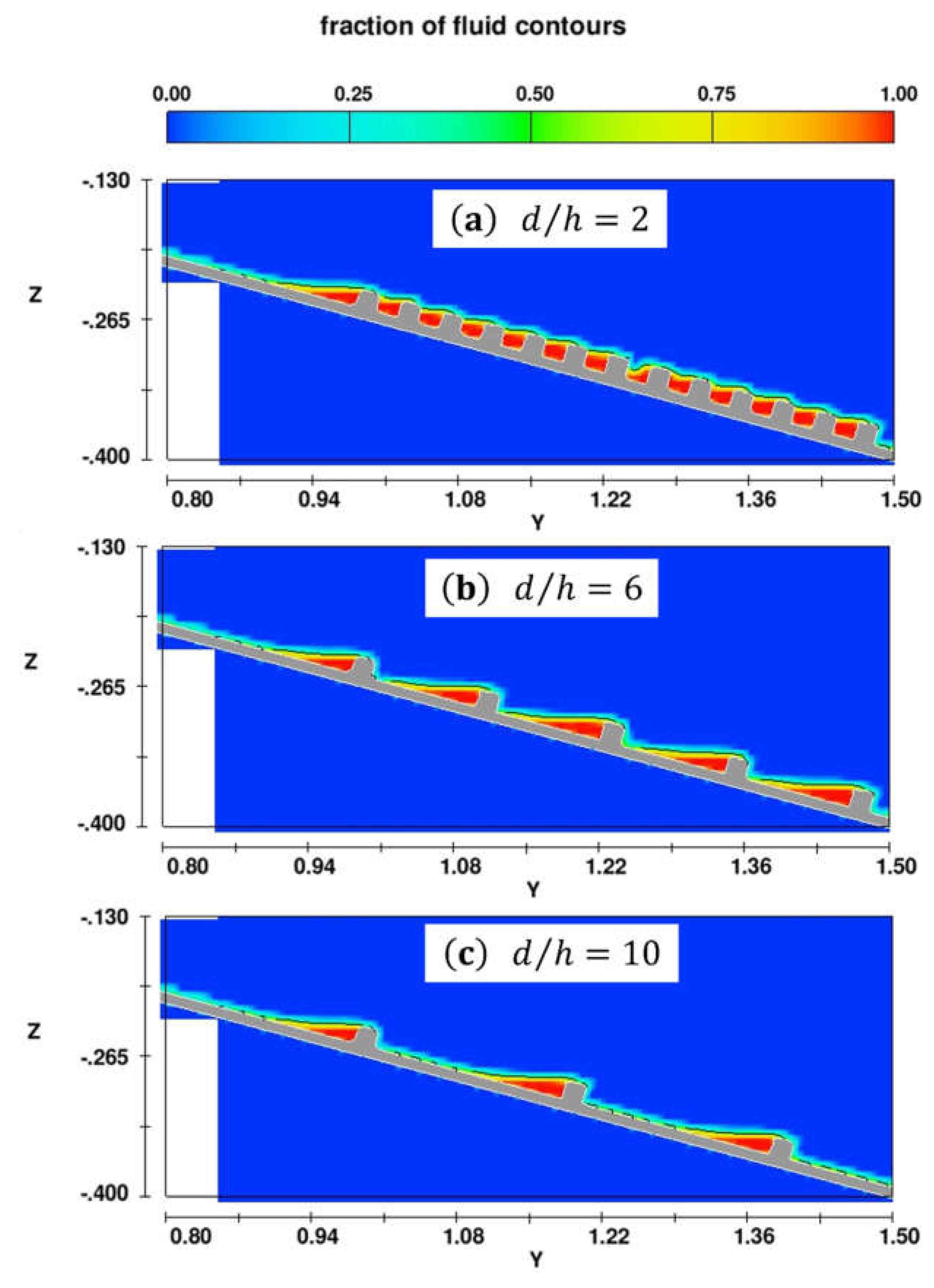
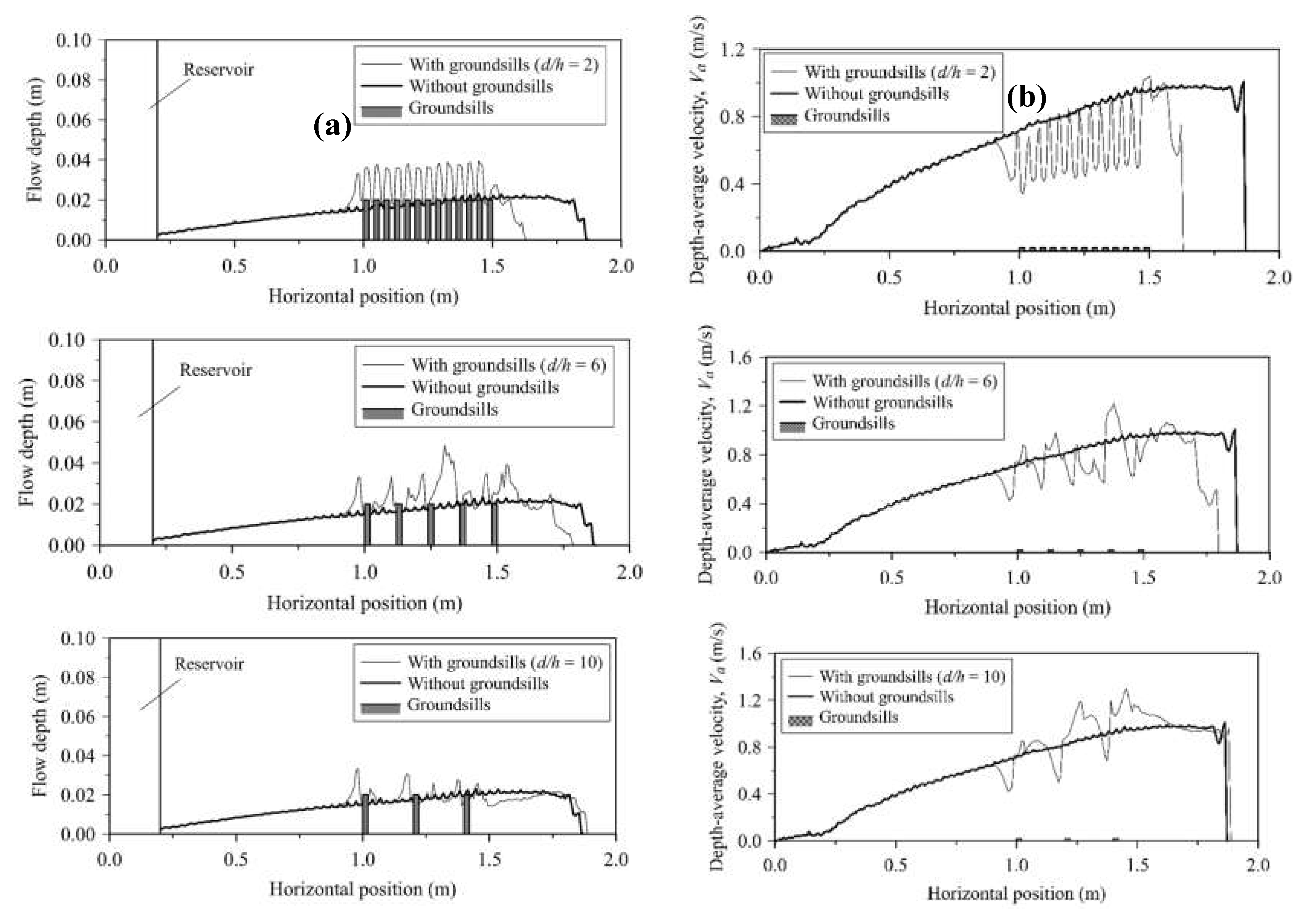
4.4. Streamwise Flow Depth and Depth-Average Velocity Profiles
Figure 11a-c presents quantitative profiles of the flow depth and depth-averaged velocity for sediment flow over different groundsill array densities. The plots compare scenarios with and without groundsills when the simulation time
. For
2, the flow depth profile exhibits oscillations corresponding to the locations of the closely spaced groundsills along the inclined channel. Compared to the case without groundsills, the presence of the groundsills introduces disturbances and fluctuations in the flow depth and velocity profiles. The velocity profile also shows variations, with localized reductions in velocity at the groundsill locations (
Figure 11a).
The fluctuations in the flow depth and velocity profiles become more evident and regular due to the increased
ratios (i.e.,
6 and 10). The magnitude of the variations in both depth and velocity is larger compared to the high array density (
2). These quantitative profiles, as illustrated in
Figure 11, support the observations made from the contour plots shown in
Figure 10, demonstrating that decreasing the groundsill array density (increasing
ratio) leads to more complex and disturbed flow patterns, with larger deviations from the unobstructed flow conditions without groundsills.
The results presented in
Figure 10 and
Figure 11 reveal an important insight: when the sediment mixture interacts with the groundsills, a dynamic interaction occurs, resulting in a hydraulic jump-like flow pattern. The formation of these hydraulic jump-like flows is a result of the interaction between the sediment mixture and the groundsills. This phenomenon demonstrates the significant impact of the groundsill obstructions on the total hydraulic behavior of the propagating sediment mixture flow.
One of the key observations from
Figure 10 and
Figure 11 is that the groundsills act as barriers, disrupting the continuous flow and causing a rapid change in the flow regime. This change is characterized by an increase in flow depth and a reduction in velocity. As the sediment mixture approaches each groundsill, the flow depth is relatively shallow, indicating a supercritical flow regime with higher velocity. Upon reaching the groundsill, the obstruction causes a sudden rise in the flow depth, producing a hydraulic jump-like flow pattern. This abrupt change in flow depth is accompanied by a dissipation of energy and a decrease in flow velocity, transitioning the flow to a subcritical regime.
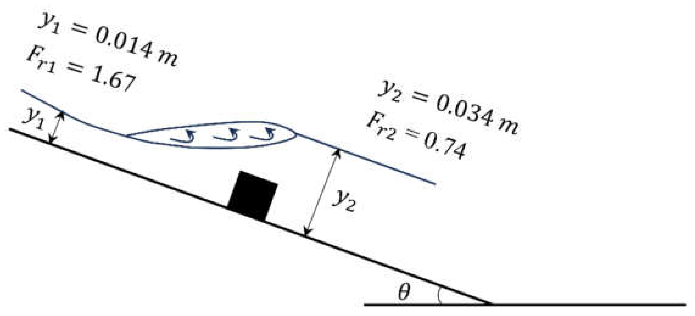
4.5. Formation of Hydraulic Jump-Like Flows Near the Groundsill
The analysis of the flow depth (
Figure 11a) and velocity profiles (
Figure 11b) provides further insights into the formation of hydraulic jumps. Along the inclined channel at
m, the average approach flow depth (
) for sediment flow approaching the first groundsill is observed to be
m. Conversely, the average post-jump flow depth (
) found to be 0.030 m (
Table 2). This increase in post-jump flow depth (
) is approximately
times higher than the approach flow depth (
), revealing the presence of hydraulic jumps.
Alternatively, the depth-averaged velocity obtained from the simulation, allows us to determine the Froude number for the flow approaching the groundsill (
) and the flow after the hydraulic jump (
). The parameters obtained for approach flow and post-jump flow are termed the approach flow parameters (
, and
) and post-jump flow parameters (
, and
), as shown in
Table 2. The approach flow parameters include the approach flow depth (
), approach velocity (
), and Froude number (
) of the flow approaching the groundsill. Similarly, the post-jump flow parameters include the post-jump flow depth (
), post-jump flow velocity (
), and post-jump Froude number (
). The terms “approach” and “post-jump” characterize the flow conditions before and after the hydraulic jump occurs.
The observed approach flow parameters and post-jump flow parameters are presented in
Table 2, showing that the values of the average
and
are
and
, respectively. This significant decrease in the Froude numbers indicates a transition from a supercritical flow regime (
) before the groundsill to a subcritical flow regime (
) after the first groundsill. This transition is evidence of a hydraulic jump-like flow occurring at the location of the groundsill, as schematically illustrated in
Figure 12.
The fact that sediment flow front flowing over low array density groundsills travels faster than the cases without groundsills, as can be seen in
Figure 9,
Figure 10 and
Figure 11, can be attributed to the increased local velocities induced by the spacing between groundsill arrays. In the context of sediment mixture propagation over groundsill arrays, lower array densities correspond to higher
ratios, indicating that the groundsills are spaced farther apart relative to their height. This configuration leads to less obstructed flow conditions, with larger spacing between the groundsills (Choi et al., 2018). While the overall flow is less impeded by these fewer obstructions, resulting in smoother propagation on average, the larger spacing between groundsills can create localized acceleration and higher velocities in certain regions (Ng et al., 2014). As the sediment flow encounters these larger openings, the lack of confinement can cause the flow to accelerate through these unobstructed sections, potentially resulting in faster front propagation over short time intervals. This phenomenon can be attributed to the principles of fluid dynamics and the conservation of mass and momentum. When the flow is less constricted, with larger cross-sectional areas available, the debris flow can accelerate to maintain continuity and conserve momentum, leading to localized increases in velocity (Jacob et al., 2005).
At a lower
ratio, the sediment mixtures tend to accumulate uniformly between the two consecutive groundsills and this can be explained by the fact that lower array densities correspond to dissipate energy and promote more uniform sediment deposition (Takahashi, 2007). As the spacing between obstacles increases, sediment mixtures tend to bypass the intermediate areas and concentrate around the groundsills (
Figure 9), resulting in non-uniform sediment deposition. When obstacles are spaced farther apart, the flow can develop enough momentum between them to maintain its speed. This allows the flow to jump from one obstacle to the next, resulting in sediment being deposited primarily near the obstacles rather than in the spaces between them, where the flow remains relatively undisturbed (Armanini and Gregoretti, 2000). The findings and analysis presented in this study are based primarily on numerical experiments of single-phase fluids, using a controlled setup with constant channel slope and groundsill dimensions. This setup allows us to gain valuable insights into the flow behavior of sediment mixtures flowing over varying groundsill array density, which can enhance our understanding of debris flow behavior in real-world scenarios. However, it did not include practical flume experiments or account for the interaction between solid phases like pebbles and the flow-bed dynamics. Future works are recommended to explore these aspects, including comprehensive simulations involving fluid-solid coupling and validation through real-world applications, to refine the design and operational strategies for groundsills.
5. Conclusions
In this study, we numerically investigate the behavior of sediment mixture with a sample volume of 2 liters flowing over arrays of groundsills installed in a laboratory-scale inclined channel with a fixed slope of . The sediment mixture is modeled as the debris flow that follows the Bingham Fluid Model, characterized by two rheological parameters: Bingham yield stress () and Bingham viscosity (). Using the commercial CFD software Flow-3D, we simulate the sediment flow over groundsill arrays with varying densities, represented by the ratio of spacing () and a fixed groundsill height ( = 0.02 m). Specifically, the array densities vary between and . The key findings are:
1. Increasing groundsill array density significantly obstructed sediment mixture propagation, reducing the flow front velocity and causing a portion of the mixture to accumulate behind the closely spaced groundsills.
2. High array density () exhibited smoother flow over the groundsills initially but transitioned to more wavy flow profiles with more flow interaction at later times.
3. Low array density () allowed free propagation but induced irregular flow patterns and fluctuating depth and velocity profiles from the start due to larger spacing between groundsills.
4. The interaction between the propagating sediment mixture and the groundsill array resulted in a hydraulic jump-like flow pattern near the groundsills. The flow depths at the location of the first groundsill were observed to be approximately times higher than the approaching flow depths.
Overall, modifying the groundsill array density provides a potential mitigation strategy by obstructing and slowing debris flows while dissipating energy through induced turbulence and wave-like patterns. High array density best restricts initial propagation, while low array arrays promote dissipation over longer runouts. Further investigations are recommended to study the effects of varying sediment mixture volumes, and different channel slope conditions on the flow behavior when encountering obstructions like groundsills. The insights obtained from this study could guide the strategic design and placement of groundsill arrays for effectively reducing debris flow mobility and mitigating related hazards.
Acknowledgments
The authors acknowledge the financial support provided by the National Science and Technology Council of Taiwan through research grants NSTC 111-2221-E-006-044-MY2.
References
- “Brookfield DV-III Ultra Programmable Rheometer Operating Instructions.” Manual No. M/98-211-A0701.
- “Flow Science Inc. (2008). FLOW-3D User’s Manual. 9.3 ed. Flow Science Inc, Los Alamos.”.
- Ancey, C., and Jorrot, H. (2001). “Yield stress for particle suspensions within a clay dispersion.” Journal of Rheology, 45(2), 297-319. [CrossRef]
- Armanini, A., and Gregoretti, C. (2000). “Triggering of debris-flow by overland flow: A comparison between theoretical and experimental results.” Proc., Debris-flow hazards mitigation: mechanics, prediction and assessment, 117-124.
- Bagli, S. P. (2019). “Challenges in Design and Construction of Embankments and Pavements, paper presented at Geotechnics for Transportation Infrastructure: Recent Developments, Upcoming Technologies and New Concepts.” Volume 1, Springer.
- Bigham, K. A. (2020). “Streambank stabilization design, research, and monitoring: The current state and future needs.” Transactions of the ASABE, 63(2), 351-387. [CrossRef]
- Britter, R., and Linden, P. (1980). “The motion of the front of a gravity current travelling down an incline.” Journal of Fluid Mechanics, 99(3), 531-543. [CrossRef]
- Choi, S. K., Lee, J. M., and Kwon, T. H. (2018). “Effect of slit-type barrier on characteristics of water-dominant debris flows: small-scale physical modeling.” Landslides, 15(1), 111-122. [CrossRef]
- De Blasio, F. V. (2011). “Introduction to the physics of landslides: lecture notes on the dynamics of mass wasting.” Springer Science & Business Media.
- Dey, L., Jan, C. D., and Wang, J. S. (2021). “Effects of particle fractions on the Bingham yield stress and viscosity of fine-coarse particle suspensions.” Journal of Mountain Science, 18(10). [CrossRef]
- Dey, L., Wang, J. S., and Jan, C. D. (2022). “Relationship among yield stress, slump, and slump flow of sediment slurries.” Journal of Chinese Soil and Water Conservation, 53(3), 167-175 (in Chinese).
- Hairani, A., and Legono, D. (2016). “Laboratory Study on Comparison of the Scour Depth and Scour Length of Groundsill with the Opening and Groundsill without the Opening.” Journal of the Civil Engineering Forum Vol. 2 (1). [CrossRef]
- Han, Z., Chen, G., Li, Y., and He, Y. (2015). “Assessing entrainment of bed material in a debris-flow event: a theoretical approach incorporating Monte Carlo method.” Earth Surface Processes and Landforms, 40(14), 1877-1890. [CrossRef]
- Han, Z., Xie, W., Yang, F., Li, Y., Huang, J., Li, C., Ding, H., and Chen, G. (2024). “3D-SPH-DEM coupling simulation for the large deformation failure process of check dams under debris flow impact incorporating the nonlinear collision-constraint bond model.” Engineering Analysis with Boundary Elements, 167, 105877. [CrossRef]
- Hatcher, L., Hogg, A. J., and Woods, A. W. (2000). “The effects of drag on turbulent gravity currents.” Journal of Fluid Mechanics, 416, 297-314. [CrossRef]
- Ikhsan, J., Fujita, M., Takebayashi, H., Sulaiman, M., and Shimomisu, Y. (2009). “Concept on sustainable sand mining management in Merapi area.” Annual Journal of Hydraulic Engineering, 53, 151-156.
- Iverson, R. M. (1997). “The physics of debris flows.” Reviews of Geophysics, 35(3), 245-296. [CrossRef]
- Iverson, R. M., and Denlinger, R. P. “The physics of debris flows—a conceptual assessment.” Proc., International Symposium on Erosion and Sedimentation in the Pacific Rim, 155-165.
- Jakob, M., Hungr, O., McDougall, S., and Bovis, M. (2005). “Entrainment of material by debris flows.” Debris-Flow Hazards and Related Phenomena, 135-158.
- Jan, C. D., Yang, C. Y., Hsu, C. K., and Dey, L. (2019). “Correlation between the slump parameters and rheological parameters of debris flow.” Proc., 7th International Conference on Debris-Flow Hazards Mitigation: Mechanics, Monitoring, Modeling, and Assessment, Association of Environmental and Engineering Geologists, 323-329.
- Jan, C.D., and Chen, C.L. (2005). “Debris flows caused by typhoon Herb in Taiwan.” Chapter 21 in the book of Jakob M., and Hungr O., Debris Flow Hazards and Related Phenomena, Springer, 363– 385.
- Jan, C. D., and Dey, L. (2022). “Effects of sediment fractions on slump-flow parameters of fine-and coarse-sediment suspensions.” Journal of Non-Newtonian Fluid Mechanics, 310, 104925. [CrossRef]
- Jan, C. D., and Dey, L. (2024). “Slump-Flow Channel Test for Evaluating the Relations between Spreading and Rheological Parameters of Sediment Mixtures.” European Journal of Mechanics-B/Fluids, 106, 137-147. [CrossRef]
- Julien, P., and O’Brien, J. (2007). “Selected notes on debris flow dynamics.” Recent developments on debris flows, 144-162.
- Lin, X., Li, G., Xu, F., Zeng, K., Xue, J., Yang, W., and Wang, F. (2022). “A coupled SPH-DEM approach for modeling of free-surface debris flows.” AIP Advances, 12(12). [CrossRef]
- Lin, P., Hsieh, T., Liao, K., Wei, K., and Lin, G. (2024). “Impact Analysis of Series of Groundsills on the Fluvial Stability and Geomorphology.” Copernicus Meetings.
- Major, J. J., and Pierson, T. C. (1992). “Debris Flow Rheology - Experimental-Analysis of Fine-Grained Slurries.” Water Resources Research, 28(3), 841-857.
- Marino, B., and Thomas, L. (2002). “Spreading of a gravity current over a permeable surface.” Journal of Hydraulic Engineering, 128(5), 527-533. [CrossRef]
- Mitschka, P. (1982). “Simple conversion of Brookfield RVT readings into viscosity functions.” Rheologica Acta, 21(2), 207-209. [CrossRef]
- Ng, C. W. W., Choi, C., Kwan, J., Koo, R., Shiu, H., and Ho, K. (2014). “Effects of baffle transverse blockage on landslide debris impedance.” Procedia Earth and Planetary Science, 9, 3-13. [CrossRef]
- Pierson, T. C. (2020). “Flow behavior of channelized debris flows, Mount St. Helens, Washington.” Hillslope processes, Routledge, 269-296.
- Rouse, H. (1965). “Critical analysis of open-channel resistance.” Journal of the Hydraulics Division, 91(4), 1-23. [CrossRef]
- Sand-Jensen, K. A. J. (1998). “Influence of submerged macrophytes on sediment composition and near-bed flow in lowland streams.” Freshwater Biology, 39(4), 663-679. [CrossRef]
- Shima, J., Moriyama, H., Kokuryo, H., Ishikawa, N., and Mizuyama, T. (2016). “Prevention and mitigation of debris flow hazards by using steel open-type sabo dams.” International Journal of Erosion Control Engineering, 9(3), 135-144. [CrossRef]
- Takahashi, T. (2007). Debris flow: mechanics, prediction and countermeasures, Taylor & Francis.
- Tsunetaka, H., Norifumi, H., Sakai, Y., Nishighchi, Y., and Hina, J. (2019). “Experimental examination for influence of debris-flow hydrograph on development processes of debris-flow fan.” Association of Environmental and Engineering Geologists; special publication 28.
- Uchida, T., Nishiguchi, Y., McArdell, B. W., and Satofuka, Y. (2019). “Numerical simulation for evaluating the phase-shift of fine sediment in stony debris flows.” Association of Environmental and Engineering Geologists; special publication 28.
- Wu, C.S. (2022). “Density-driven exchange flow propagating over an array of densified obstacles.” Physics of Fluids, 34(11). [CrossRef]
Figure 1.
A series of check dams (groundsills) constructed in a debris flow gully in Hualien County, Taiwan.
Figure 1.
A series of check dams (groundsills) constructed in a debris flow gully in Hualien County, Taiwan.
Figure 2.
Particle size distribution curve of the clay-silt materials used as sediment in the rheometer tests.
Figure 2.
Particle size distribution curve of the clay-silt materials used as sediment in the rheometer tests.
Figure 3.
(a) Schematic diagram illustrating the rheological measurement setup using a rotational rheometer (Dey et al., 2021), (b) Rheological characteristics of the sediment mixture with .
Figure 3.
(a) Schematic diagram illustrating the rheological measurement setup using a rotational rheometer (Dey et al., 2021), (b) Rheological characteristics of the sediment mixture with .
Figure 4.
Schematic diagrams of the experimental setup for simulating sediment mixture flow over a beam-type array of groundsills in an inclined channel: (a) side view and (b) top view at a fixed channel slope, .
Figure 4.
Schematic diagrams of the experimental setup for simulating sediment mixture flow over a beam-type array of groundsills in an inclined channel: (a) side view and (b) top view at a fixed channel slope, .
Figure 5.
Illustrations of beam-type groundsill arrays with (a) high array density (closely spaced groundsills), (b) low array density (widely spaced groundsills) in 2D and 3D, and (c) Schematic diagram for the relation between and channel slope, .
Figure 5.
Illustrations of beam-type groundsill arrays with (a) high array density (closely spaced groundsills), (b) low array density (widely spaced groundsills) in 2D and 3D, and (c) Schematic diagram for the relation between and channel slope, .
Figure 6.
Configuration of the numerical model domain for simulating flow over an array of groundsills at a fixed slope: (a) boundary conditions, and (b) computational mesh.
Figure 6.
Configuration of the numerical model domain for simulating flow over an array of groundsills at a fixed slope: (a) boundary conditions, and (b) computational mesh.
Figure 7.
Visualization of the instantaneous velocity magnitude of sediment mixtures propagating over a low array density (specifically, ) of groundsills at different simulation times.
Figure 7.
Visualization of the instantaneous velocity magnitude of sediment mixtures propagating over a low array density (specifically, ) of groundsills at different simulation times.
Figure 8.
Temporal evolution of the front position of sediment mixtures for varying groundsill array densities.
Figure 8.
Temporal evolution of the front position of sediment mixtures for varying groundsill array densities.
Figure 9.
Contour plots of sediment mixture fraction at simulation times of 0.7, 1.0, and 1.5 s for flow over groundsill arrays with densities of (a) , (b) , (c) , (d) , and (c) .
Figure 9.
Contour plots of sediment mixture fraction at simulation times of 0.7, 1.0, and 1.5 s for flow over groundsill arrays with densities of (a) , (b) , (c) , (d) , and (c) .
Figure 10.
Contour plots of sediment mixture fraction at simulation times for flow over groundsill arrays with densities of , , and .
Figure 10.
Contour plots of sediment mixture fraction at simulation times for flow over groundsill arrays with densities of , , and .
Figure 11.
Streamwise profiles of (a) flow depth and (b) depth-averaged velocity of sediment mixtures propagating over groundsill arrays at , comparing cases with and without groundsills for different array densities.
Figure 11.
Streamwise profiles of (a) flow depth and (b) depth-averaged velocity of sediment mixtures propagating over groundsill arrays at , comparing cases with and without groundsills for different array densities.
Figure 12.
Schematic representation of the formation of hydraulic jump-like flows at the first groundsill for array density .
Figure 12.
Schematic representation of the formation of hydraulic jump-like flows at the first groundsill for array density .
Table 1.
Groundsill array densities and number of groundsills installed in the specific channel reach.
Table 1.
Groundsill array densities and number of groundsills installed in the specific channel reach.
| Simulation No. |
Array density,
|
Spacing, (m) |
No. of groundsills |
| S1 |
2 |
0.04 |
13 |
| S2 |
4 |
0.08 |
7 |
| S3 |
6 |
0.12 |
5 |
| S4 |
8 |
0.16 |
4 |
| S5 |
10 |
0.20 |
3 |
Table 2.
Flow parameters obtained through simulation for sediment mixture approaching and flowing over the first groundsill when
Table 2.
Flow parameters obtained through simulation for sediment mixture approaching and flowing over the first groundsill when
| Array density() |
Approach flow parameters |
Post-jump flow parameters |
|
(m) |
(m/s) |
|
(m) |
(m/s) |
|
| 2 |
0.015 |
0.65 |
1.69 |
0.032 |
0.42 |
0.75 |
| 4 |
0.014 |
0.62 |
1.67 |
0.034 |
0.43 |
0.74 |
| 6 |
0.014 |
0.64 |
1.73 |
0.033 |
0.47 |
0.83 |
| 8 |
0.015 |
0.63 |
1.64 |
0.033 |
0.46 |
0.81 |
| 10 |
0.014 |
0.63 |
1.70 |
0.033 |
0.46 |
0.81 |
| Average |
0.014 |
0.63 |
1.67 |
0.030 |
0.45 |
0.79 |
|
Disclaimer/Publisher’s Note: The statements, opinions and data contained in all publications are solely those of the individual author(s) and contributor(s) and not of MDPI and/or the editor(s). MDPI and/or the editor(s) disclaim responsibility for any injury to people or property resulting from any ideas, methods, instructions or products referred to in the content. |
© 2024 by the authors. Licensee MDPI, Basel, Switzerland. This article is an open access article distributed under the terms and conditions of the Creative Commons Attribution (CC BY) license (http://creativecommons.org/licenses/by/4.0/).