
Submitted:
16 December 2024
Posted:
17 December 2024
You are already at the latest version
Abstract
This paper deals with the axial crushing characteristics of sandwich cylinders with a BCClattice core based on the nonlinear finite element (FE) method. In particular, the effect ofcore and cylinder diameter on the crushing characteristics were investigated. By introducingthe lattice core sandwiched between two tubes, the deformation behaviour can be controlledaxisymmetrically, leading to an increase in the average load Pave, due to the local bendingresistance. In addition, a series of lattice sandwich tubes were fabricated using a metal 3Dprinter, and their axial compressive responses were compared with the FE analysis, where goodagreement was observed.
Keywords:
Crushworthiness
; Cylindrical tube
; Lattice core
; Axial compression test
; FEM
1. Introduction
In recent years, thin-walled tubes for use as impact energy absorption devices, have been investigated by many researchers, and a wide range of cross-sectional and longitudinal shapes have been proposed for enhancing their absorption capacity [1,2,3,4,5,6,7,8]. These structures have been widely used in numerous engineering fields, such as the aerospace, nautical, automobile and rail sectors. In general, thin-walled tubes are made of lightweight metals, fibre reinforced plastics as well as hybrids of the two [8]. In addition, sandwich composite materials, composed of two thin face sheets and a low-density core, such as foams and honeycombs , have received much attention recently, due to advances in manufacturing technology, and their energy absorption capability has been studied by many researchers [9,10,11,12,13,14,15,16,17]. For example, Zhu et al. [18] conducted axial and lateral compression tests on square corrugated sandwich tubes in which the corrugated core and outer square tube were fabricated using a hot press molding method. Also, Fan et al. [19] and Li et al. [20] fabricated sandwich cylinders with two-dimensional periodic cores, and conducted axial compression tests to evaluate their energy absorption capacity. Moreover, Sun et al. [21] proposed a theoretical model based on equivalent monocoque shell theory to predict the mechanical behaviour of composite sandwich cylinders with 2D lattice cores under axial compression. A lattice core is widely recognized as an open-cellular structure, and many papers have been published on the mechanical response of lattice structures [21,22,23,24,25,26].
In recent years, novel sandwich structures, composed of more precise periodical cellular cores, such as 3D lattices, have been produced, and their mechanical properties have been investigated by many researchers [27,28,29,30,31,32,33,34]. These advances can be attributed to the rapid development and widespread use of additive manufacturing technology. For example, 3D printers for metals, which is recognized as a subset of additive manufacturing technology, have been introduced onto the market, and many structural components with more precise and complex shapes can now be fabricated easily. One of the more common structural components fabricated by metal 3D printers is a micro-lattice structure. This structure is composed of slender strands with a length scale of micrometres, connecting periodically in 3D space. One of the authors has investigated the mechanical properties of lattice blocks subjected to uniaxial compression and shear loading [28,29]. Also, the structural and vibrational response of composite sandwich panels and cylinders based on lattice cores has been studied and reported [16,18,19,20,21,32,33,34].
In this study, the axial compressive response of composite lattice tubes has been studied using a non-linear FE method. In particular, the effects of core micro-architecture on the initial and average peak loads sustained by the tube as well as the deformation behaviour are discussed. The lattice core discussed in this study is composed of a body-centred cubic (BCC) unit-cell The unit cell has eight slender strands connected to each other at the centre of a cube. The BCC architecture is not optimal, but has the advantages of being easy of manufacture. Finally, compression tests on the tubes have been conducted, and the accuracy of the FE analysis is discussed. Due to the periodic, precise and complex micro-architecture of a lattice core, we believe that the lattice-cored sandwich tube could result in lightweight components that possess higher energy dissipation, coupled with microwave absorption and heat transfer properties for use in land transport, aerospace and many kinds of applications. The advantage of this tube is an ease of manufacture and applicability of optimization for the micro-architecture.
The main contribution of the study is as follows:
- An effective FE procedure for modelling the compressive response of a lattice-cored sandwich tube is proposed.
- It is shown that by sandwiching the lattice core between two cylinders, the deformation behaviour can be controlled axisymmetrically. The observed wrinkle length is approximately equal to the length of the lattice unit-cell.
- The average stress in a sandwich tube is presented as a function of the equivalent wall thickness ratio and the relative density of the core .
- A series of lattice sandwich tubes fabricated using a metal 3D printer have been tested, and it has been shown that their axial compressive response agrees well with the FE results.
2. Analysis Methods
In this study, an elastoplastic numerical analysis of a sandwich tube subjected to an axial compressive displacement is conducted using the commercial FE analysis software MSC.Marc.2023. A schematic illustration of the numerical model of the sandwich tube is shown in Figure 1(a). Regarding the boundary conditions, the lower end of the tube was fixed, and a rigid plate was displaced quasi-statically to contact from the upper surface of the tube. Once the rigid plate was touched the tube end, the nodes on the tube edge were glued to the plate, and no slip movements were not allowed. Figure 1(b) shows a schematic diagram of the cylindrical model viewed in the transverse plane (-plane). The sandwich tube is a structure in which a lattice core is arranged in a concentric circle, being sandwiched between two tubes. The unit cell of the lattice core consists of eight identical slender strands connected firmly, as shown in Figure 1(c). The diameter of the strands is given as . In this paper, we refer to the lattice core as a body centred cubic (BCC) structure. The unit-cell of a BCC is shown in Figure 1(c). The parameters and in Figure 1(c) represent the length of the unit cell and the opening angle, respectively. Here, the angle, , was set to in order to maintain the shape of the unit cell as cubic. Also, the axial length, L, of the tube was set to a constant value (50 mm), and the thickness of the tube, h, was set to 0.4 mm. In addition, the radius, R, is defined as the distance from the centre of the structure to the surface of the inner tube, and the diameter, D, was set to . Table 1 summarises the values and the ranges of the geometrical parameters of the sandwich tube. The values and were selected to reflect the actual values that can be manufactured by our in-house metal 3D printer. In this paper, the effects of geometrical parameters on the crushing characteristics of sandwich lattice tubes are investigated systematically.

Table 1.
Dimensions of the lattice-sandwich tube model
| Tube length L[mm] | 50 |
| Tube thickness h[mm] | 0.4 |
| Inner tube radius R[mm] | 15∼40 |
| Core length [mm] | 2.5, 5.0 |
| Lattice diameter [mm] | 0.2∼0.3 |
In the following section, the element types and the number of element divisions that were adopted in the FE analysis are described. The strands in the BCC lattice were discretized using two-noded beam elements. All of the strands were divided into 10 beam elements in order to minimize the effect of element size on the end result. Also, four-noded thick-walled shell elements were selected to model the cylindrical part, which was divided into 36 elements () in each BCC unit cell (see Figure 1(c)). No significant effect of element size on the axial crushing characteristics of the lattice-cored sandwich tubes was observed by varying the number of divisions. In addition, all of the degrees of freedom (DOF) at the connection points between the shell element of tubes and the beam elements of the lattice core are shared, and the rotational movements at the connection points are constrained.
As a contact condition, the offset function was activated between the rigid plate and the cylindrical part that reflects the actual thickness of the tube. Also, a self-contact function, in which the offset distance between strands is equal to the strand diameter , was applied to all strands.
In addition, an adhesive contact condition was applied between the upper rigid plate and the cylindrical tube, as well as a touching contact condition between the lower rigid plate and the cylindrical model. Frictional forces were ignored. Figure 1(d) shows a photograph of a sandwich tube following manufacture in the metal 3D printer.
Next, we will describe the material properties adopted in the numerical simulation. It is assumed that these structures behave as if based on a homogeneous and isotropic elastoplastic material with a Von Mises yielding condition. The stress-strain relationship can be expressed in the following manner;
Here, E, and represent the Young’s modulus, strain hardening coefficient and the initial yield stress, respectively. In this study, it is assumed that the lattice-sandwich tube is made of stainless steel (SUS630), and the tube is fabricated by a metal 3D printer. Based on an earlier study, the values of the Young’s modulus E and the initial yield stress for a tensile specimen fabricated by a metal 3D printer were measured from a quasi-static tensile test, and their values (E=182GPa and =525MPa) are applied in our calculation. Also in our calculation, the strain hardening coefficient was taken as . In the current numerical study, the updated Lagrange method was used to formulate the geometric nonlinear behaviour, and the Newton-Raphson method as well as the return-mapping method, were used to solve the nonlinear equation.
3. Results
3.1. Influence of the Lattice core on the Observed Wrinkle Length
In this section, the influence of the lattice core sandwiched between the two tubes on the axial crushing behaviour of the cylindrical sandwich structure is discussed. Prior to this, we have also investigated the compressive response of thin-walled hollow tubes that consist of inner and outer circular tubes without a lattice core, and have evaluated the initial peak load and the average load and subsequently compared these values with analytical results in order to verify the effectiveness of our numerical simulation, as well as to clarify the role of the lattice core in the energy absorption process. Many papers have been published regarding the axial compressive response of thin-walled circular tubes, and some analytical equations have been proposed for estimating the initial peak load and the average load . Here, the peak load, , corresponds to the initiation of local plastic bending near the fixed end. Also, the average load, , is determined from the mean value of the compressive load up to the point at which half of the tube is crushed, namely,
For example, Chen et al. [3] predicted the initial peak load for a circular tube using an FE analysis, and showed that can be written as:
Here, the parameters and depend on the material properties and tube geometry, and are given by:
Also, Wierzbicki [35] proposed an empirical equation for the average load Pave as:
Table 2 shows the values of the peak load, , and the average load, , for two kinds of hollow tube under axial compression obtained by our FE analyses. Table 2 also includes the predictions derived from Eqs.(3) and (5). In the table, the numbers following the character R represent the radius values of the inner and outer tubes. For example, the model (+) consists of two tubes, in which the radius of the inner tube is 30mm, and that for the outer tube is 32.5mm. Regarding the predictions of the loads and , since each structure is composed of two tubes, two sets of and values can be calculated from the predictions (Eqs.(3) and (5)). We have summed them up and present the values in Table 2. It can be seen in Table 2 that their predictions agree reasonably well with the FE results, regardless of the combinations of tube radius R.
Table 2.
Comparison of peak and average loads and obtained by FEM analysis and previously-proposed equations
Table 2.
Comparison of peak and average loads and obtained by FEM analysis and previously-proposed equations
| model | [kN] | [kN] | ||||
| FEM | Eq.(3) | relative error[%] | FEM | Eq.(5) | relative error[%] | |
| R30+R32.5 | 80.3 | 82.7 | 3.0 | 16.6 | 16.4 | 0.8 |
| R30+R35 | 86.3 | 86.0 | 0.3 | 17.9 | 16.6 | 7.7 |
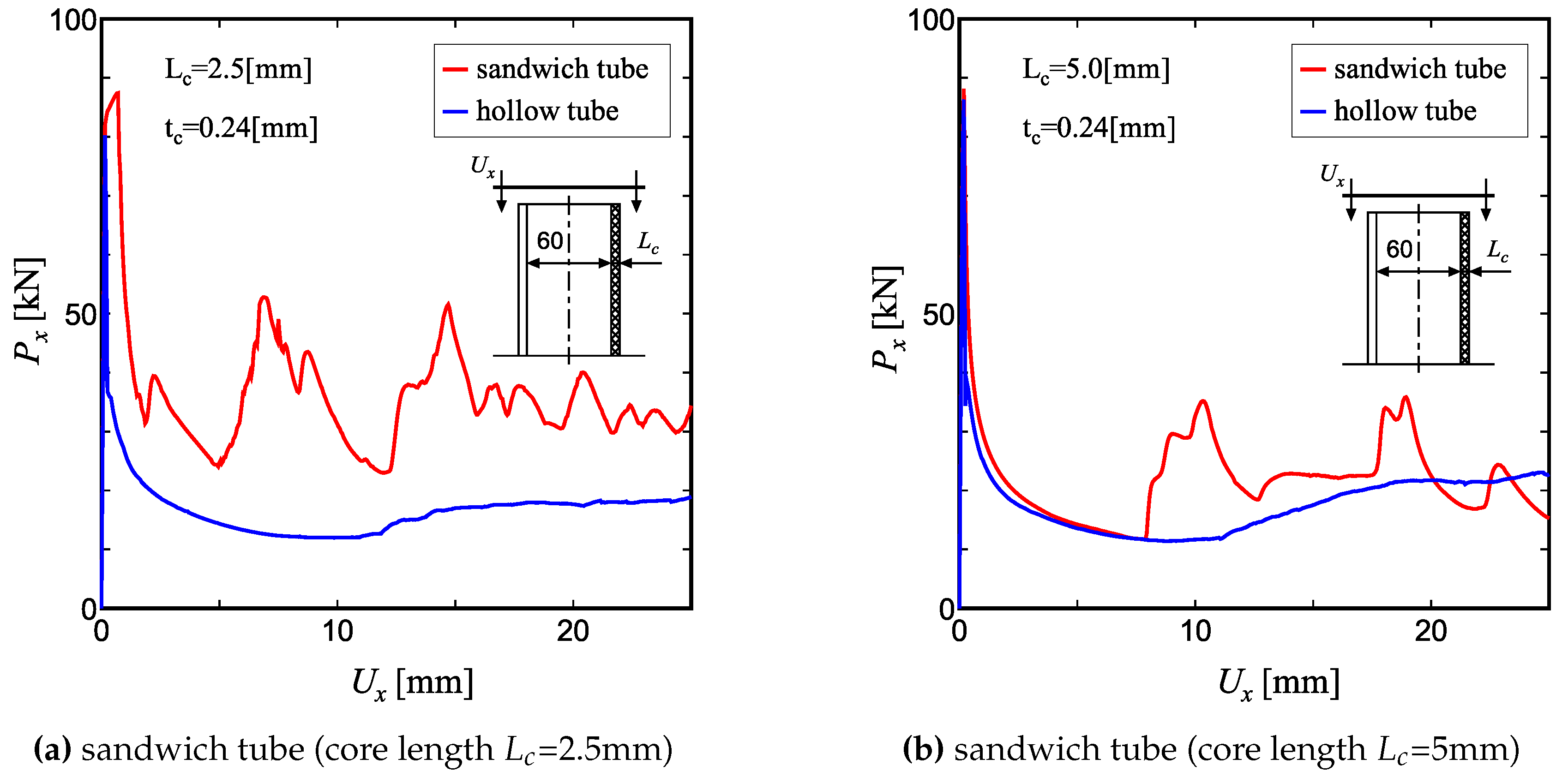
Figures 2 (a) and (b) show the variation of the axial compression load for circular tubes with and without lattice cores. The results for the tubes with lattice cores are denoted by red curves, and those without lattice cores are shown by blue curves. Here, the inner diameter of the tube was set to a common value (60mm) for all tubes, and two values of outer diameter were employed in the FE model. The lattice core was introduced between the inner and outer shells. Here, two kinds of lattice core length, with =2.5mm and 5.0mm were selected, and their contributions to the compressive load are discussed. These figures show how the lattice core affects the compressive load-carrying capacity, and also demonstrate that a finer lattice core is more effective for improving properties. It can be seen from these figures that the lattice core does not affect the initial peak load, but enhances the average load following the peak load. This is due to the fact that since the lattice core is softer than the surrounding cylindrical shell, the failure behaviour up to the peak load is independent of core geometry. It does, however, improve the folding behaviour of the wrinkles. As a result, the fluctuating load behaviour is enhanced and the load-carrying capacity is improved. This is especially the case when the core thickness =2.5mm, where the contribution becomes significant. Figure 3(a) and (b) compare the deformed shapes of tubes based on different core sizes (=2.5mm and 5.0mm) subjected to an axial displacement =0.5. For comparison, the deformed shapes of a double tube without a lattice core is also shown in Figure 4(a) and (b). It is evident from these figures that the wrinkle folding distance during crushing is reduced by inserting the lattice core, and the deformation behaviour during crushing is axisymmetric.
Figure 2.
Comparison of compressive load-displacement curve for a hollow tube and a sandwich tube
In the following, we will discuss the effect of varying the lattice core geometry on the observed wrinkle length. Here, the following equation is used to estimate the relative density of the lattice core:
This equation can be readily derived by considering the volume ratio of the lattice strands in a cubic-shaped lattice core (see Figure 1(c)). Figure 5(a) shows a comparison of the compressive load versus deflection curve and Figure 5(b) shows the deformed shape when the displacement =0.5 for lattice sandwich tubes based on two different core sizes but having the same strand diameter =0.24mm. Also, Figure 6(a) and (b) show similar results for lattice tubes based on the same relative density, that is =0.035. Here, in order to make it easier to observe the folding patterns, the deformed shapes shown in Figure 5(b) and 6(b), correspond to the outline of the the outer surface of the tube. The index x in Figure 5(b) and Figure 6(b) represents the axial coordinate and the index y represents the radial coordinate of the cylinder. As can be seen in Figure 5(b) and Figure 6(b), the wrinkle length is strongly dependent on the lattice core length , with the wrinkle for =2.5mm being shorter than that for =5.0mm. This clearly indicates that a shorter wrinkle length is associated with a higher energy absorption capacity.
3.2. Evaluation of Energy Absorption Performance via the Maximum Crush Displacement and the Average Load )
The total amount of energy absorbed by the lattice tubes during axial compression, W, can be calculated by multiplying the maximum displacement , and the average load , as shown in Equation (7)
Figures 7(a) and (b) show the load-displacement traces until the load increases dramatically for sandwich tubes with =2.5 mm and 5.0 mm. Here, the maximum displacement is defined as the axial displacement at the point where the load suddenly increases, and is shown by the dashed lines in Figure 7(a) and Figure 7(b).
Figure 7(a) shows the results for the same strand diameter =0.24mm, Also, Figure 7(b) shows the results for the same relative density =0.035. It can be seen from Figure 7(a) that the difference in the maximum displacement , due to the difference in the core length , is negligible for the same strand diameter . Similarly, it can be seen in Figure 7(b) that the difference in due to changes in the core length is also negligible for the same relative density of core . Therefore, it can be concluded that the core length has little influence on the maximum displacement during crushing.
Table 3 shows the ratio of the maximum displacement and the average load during crushing and the absorbed energy W of the model used in Figure 7(a) and (b) for cases of =2.5mm and =5.0mm. In the table, , and represent the maximum displacement, the average load and the absorbed energy for =2.5mm, and , and shows those for =5.0mm. It can be seen from this table that the ratio of absorbed energy is always greater than 1, regardless of the strand diameter and the relative density . Therefore, it can be concluded that the sandwich tube with the core of =2.5mm, which has a smaller cell size, offers superior crushing characteristics to that based on a larger cell size of =5.0 mm.
Table 3.
Comparisons of maximum deflection , average load and absorbed energy W for the lattice sandwich tubes
Table 3.
Comparisons of maximum deflection , average load and absorbed energy W for the lattice sandwich tubes
| [mm] | [mm] | [mm] | [kN] | W[Nm] | / | / | / |
|---|---|---|---|---|---|---|---|
| 2.5 | 0.24 | 32.1 | 25.2 | 809 | 0.97 | 1.34 | 1.30 |
| 5.0 | 0.24 | 33.1 | 18.8 | 622 | |||
| 2.5 | 0.2 | 36.1 | 22.6 | 815 | 1.02 | 1.09 | 1.11 |
| 5.0 | 0.4 | 35.4 | 20.8 | 737 |
Figure 8 shows the variation of the average stress obtained from the FE analysis with tube relative thickness . In addition, the average stress is calculated by considering the cross-sectional area of the sandwich tube. Here, the parameters and in the figure represent the equivalent thickness and radius of the sandwich tube, and they are defined as follows:
In Figure 8, two values of core length, =2.5mm and 5.0mm, were selected, where the strand diameter was set to a constant value (0.22mm), and only the tube radius R was varied. It can be seen from this figure that for each length , the average stress increases as the wall thickness ratio increases. This trend is particularly appearent for tubes with a small core length =2.5mm.
In addition, it is clear that the results for =2.5mm are always higher than those for =5.0mm, which is due to the decreased equivalent thickness associated with larger values of . In other words, as the core length becomes small, the distance between the inner and outer tubes decreases, giving a higher relative density for the same strand diameter . In contrast, when the core length is large, the density decreases for the same strand diameter . As a result, the contribution to the equivalent tube thickness decreases for larger values of . As can be seen in Figure 8, the average stress is proportional to , which is similar to that observed for a continuum single tube. Curve fits calculated using the least squares method are represented by the blue and red curves in Figure 8, which are based on the following equation:
Here. the parameter C is a constant that depends on the lattice core length , and is derived from the curve fitting based on the FE data. For example, C=5.6 for =2.5mm and C=2.0 for =5.0mm.
3.3. Relationship Between Deformation Mode and Energy Absorption W
In this section, the relationship between the observed deformation modes (axisymmetric and non-axisymmetric) of the sandwich tube and the associated energy absorption W is discussed. Figure 9 shows the deformation modes (axisymmetric and non-axisymmetric) identified in a sandwich tube with a lattice core length of =5.0mm when the tube was crushed to half of its length, classified by the tube thickness ratio and the relative density of the lattice core . The range of dimensions for the sandwich tube in the deformation mode map are mm and mm. It can be confirmed from this figure that smaller values of the thickness ratio result in the larger values of relative density of the lattice core, increasing the likelihood of axisymmetric deformation during crushing. Figure 10(a) shows the variation of the Specific Energy Absorption (SEA) with thickness ratio , where the relative density is held constant. Here, the red symbols in the figure correspond to the results under non-axisymmetric deformation, and the blue symbols show those linked to axisymmetric deformation. It is clear that as the relative wall thickness increases, the deformation behaviour changes from axisymmetric to non-axisymmetric deformation (depicted by Transition(1) in Figure 9). It can be seen from this figure that the SEA value increases as the wall thickness increases, and increases rapidly near the point where the deformation behaviour switches from axisymmetric to non-axisymmetric. In other words, for a sandwich tube with a lattice core with a given relative density, increasing the wall thickness results in an enhanced energy absorption per unit mass (SEA). However, since the wrinkle length for a non-axisymmetric deformation pattern is greater than that for axisymmetric deformation, there are more undeformed parts in the tube. Clearly, a non-axisymmetric deformation mode is an undesirable deformation response. Figure 10(b) shows the variation of SEA with the relative density for a constant the wall thickness (depicted by Transition(2) in Figure 9). As can be seen in Figure 10(b), the SEA increases as the relative density increases, and the deformation mode shifts from non-axisymmetric deformation to axisymmetric deformation. Figure 11 shows the variation of SEA as the strand diameter is varied from 0.2 to 0.3 mm, for a constant core length =2.5mm and tube radius R=15mm. As was the case in Figure 10(b), the SEA increases as the relative density of the core increases. This evidence suggests that designers can enhance the specific energy absorption (SEA) by inserting a lattice core between two thin-walled circular tubes. Designers can determine the appropriate lattice unit size by considering the maximum tube weight, tube radius and the requirements for specific absorbed energy.
3.4. Comparison with Experimental Results
In this section, the results of axial compression tests on lattice sandwich tubes fabricated using a metal 3D printer (ProX 300, 3D Systems), and the prediction of the FE analysis are compared and discussed. Firstly, we explain the experimental conditions for the axial compression tests. A part of the cylindrical specimen manufactured in the metal 3D printer is shown in Figure 12. The test machine used in this study is an INSTRON 5982. Both ends of the cylindrical specimen were fixed firmly. A photograph of the compression test is shown in Figure 13(a) and a schematic diagram is shown in Figure 13(b). The test specimens used in this experiment were based on SUS630, and the dimensions of the specimens (Shapes A∼F) are shown in Table 4. The number of samples was one each for the thin-walled cylinders and three each for the sandwich tubes (depicted by Samples 1,2,3). The effects of the inner tube diameter D and the strand diameter on loading performance and compression behaviour were investigated. The experimental conditions were quasi-static compression at a crosshead speed of m/s. The maximum displacement was set to =30mm, but for comparison with the analytical results, only values up to =25mm will be considered.
Table 4.
Summary of the geometrical parameters of the specimens for compression testing
| Specimen | L[mm] | D[mm] | h[mm] | [mm] | [mm] | coretype |
| A | 50 | 35 | 0.4 | - | - | - |
| B | 45 | |||||
| C | 55 | |||||
| D | 30 | 2.5 | 0.2 | BCC | ||
| E | 40 | |||||
| F | 50 |
The material properties for the FE analysis are based on tensile tests on SUS630 as shown in Figure 14. The load-displacement diagrams for the thin-walled single tubes with tube diameters D=35mm (Shape A), 45mm (Shape B) and 55mm (Shape C) are shown in Figure 15(a) and Figure 15(b).
The peak load and average load for each model are given in Table 5. The ratio in the table represents the ratio of the experimental value to the numerical analysis value.
Table 5.
Comparison of the experimental and predicted values of and following compression testing on the thin-walled tubes
Table 5.
Comparison of the experimental and predicted values of and following compression testing on the thin-walled tubes
| Specimen | D[mm] | [kN] | [kN] | ||||
| FEM | Experiment | EXP/FEM | FEM | Experiment | EXP/FEM | ||
| A | 35 | 23.146 | 11.630 | 0.51 | 7.195 | 4.825 | 0.68 |
| B | 45 | 29.795 | 14.658 | 0.49 | 7.273 | 4.741 | 0.65 |
| C | 55 | 35.408 | 14.092 | 0.40 | 7.850 | 5.023 | 0.64 |
By considering the compression tests and the FE data, it was found that the experimental load values, especially the peak load , were smaller than those predicted by the FE analysis. The reason for this discrepancy can be explained by the occurrence of an undesirable rotation near the fixed ends of the tubes. Also, the degree of the parallelization of the specimen edges cannot be guaranteed with a high degree of accuracy for specimens manufactured using additive manufacturing. As a result, the direction of the compression load could be inclined, and a part of the cylindrical end may deform and buckle prematurely. Thus, the initial shape of the experimental load-displacement curve is lower than that obtained from the FE analysis, and the peak load is smaller than the FE predictions. The similar tendency has also been observed and discussed for a torsional crushing behaviour of foam-filled thin-walled square columns by W. Chen et al. [36]. Figure 16 shows the comparisons of the load-displacement curve for a single tube (Shape A) under different boundary conditions for the nodes on both tube edges. In the figure,“Fixed” represents that all rotational movements around x-, y- and z-directions as well as parallel movements along all directions are constrained for the nodes on both sides. Also, “Rotate” represents that the rotational movements are only allowed. Since in the experimental machine, there is a carved groove on each touched surface to interfere parallel movement of the specimen, the latter boundary condition is closer to the actual experiment. As can be found from the figure that the calculated peak load under the “Rotate” condition is almost coincident with experimental result.
Here, the results of the compression tests and the numerical analysis are compared for a sandwich tube with a BCC lattice core, an inner tube diameter D=30mm and a strut diameter =0.2mm (Shape D). The load-displacement traces for both models are shown in Figure 17, and the peak load and the average load values for each model are given in Table 6. The ratio in the table represents the ratio between the experimental value and the average value from the numerical analysis. Figure 18 shows specimens following compression testing on two cylindrical shapes with equal outer tube diameters, a thin-walled single tube with D=35mm (Shape A) and a lattice sandwich tube with D=30mm (Shape D).
Table 6.
Comparison of the and values with numerical data from an FE analysis following experimental compression testing for a lattice sandwich tube with inner diameter D =30mm (Specimen shape D).
Table 6.
Comparison of the and values with numerical data from an FE analysis following experimental compression testing for a lattice sandwich tube with inner diameter D =30mm (Specimen shape D).
| Specimen D | [kN] | [kN] | ||||
|---|---|---|---|---|---|---|
| D=30mm, =0.2mm | FEM | EXP | EXP/FEM | FEM | EXP | EXP/FEM |
| Sample1 | 33.771 | 13.226 | ||||
| Sample2 | 45.471 | 33.073 | 0.74 | 16.727 | 14.039 | 0.82 |
| Sample3 | 33.677 | 13.984 | ||||
In the following, the results of the experimental tests and the numerical analyses are compared for a sandwich tube with a BCC lattice core with an inner tube diameter D=40mm and a strut diameter =0.2mm (Shape E). The load-displacement diagrams for both models are shown in Figure 19, and the peak load and the average load for each model are shown in Table 7. Figure 20 shows two samples with equal outer tube diameters after compression testing. Figure 20(a) shows a thin-walled single tube with D=45mm (Shape B) and Figure 20(b) shows a lattice-sandwiched tube with D=40mm (Shape E).
Table 7.
Comparison of the experimental and predicted values of and following compression testing (D=40mm, Specimen shape E)
Table 7.
Comparison of the experimental and predicted values of and following compression testing (D=40mm, Specimen shape E)
| Specimen E | [kN] | [kN] | ||||
|---|---|---|---|---|---|---|
| D=40mm, =0.2mm | FEM | EXP | EXP/FEM | FEM | EXP | EXP/FEM |
| Sample1 | 39.503 | 15.798 | ||||
| Sample2 | 59.320 | 37.878 | 0.64 | 21.075 | 15.581 | 0.76 |
| Sample3 | 37327 | 16503 | ||||
Next, the results of compression tests and the numerical analysis are compared for a sandwich tube with a BCC lattice core with an inner tube diameter D=50mm and strut diameter =0.2mm (Shape F). The load displacement traces for both models are shown in Figure 21, and the peak load and the average load values for each model are shown in Table 8. Photographs of specimens after compression testing on two cylindrical samples with equal outer tube diameters, a thin-walled single tube for which D=55mm (Shape C) and a lattice sandwich tube for which D=50mm (Shape F) are shown in Figure 22.
Table 8.
Comparison of the experimental and predicted values of and following compression testing (D =50mm, Specimen shape F)
Table 8.
Comparison of the experimental and predicted values of and following compression testing (D =50mm, Specimen shape F)
| Specimen F | [kN] | [kN] | ||||
|---|---|---|---|---|---|---|
| D=50mm, =0.2mm | FEM | EXP | EXP/FEM | FEM | EXP | EXP/FEM |
| Sample1 | 44.594 | 17.805 | ||||
| Sample2 | 72.903 | 42.285 | 0.59 | 25982 | 17927 | 0.68 |
| Sample3 | 42.947 | 17.584 | ||||
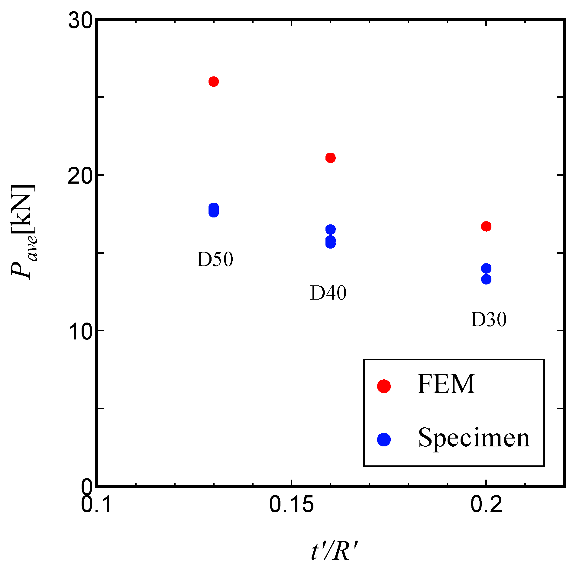
From these results, it can be seen that the deformation behaviour of the tube under axial compression testing can be controlled in an axisymmetric mode by introducing a lattice core, and that the load increased and decreased due to the generation of wrinkles during compression. In the case of the sandwich tubes, there is an error between the experimental load values and the predicted values, but the cause of this error is considered to be the same as in the case of thin-walled single cylinders. Figure 23 shows the variation of Pave with the wall thickness ratio for lattice cylinders with values of D equal to 30, 40 and 50mm. Included in the figure are both the experimental data and the numerical predictions. As a result, as the cylindrical wall thickness ratio decreases, i.e., as the inner tube diameter D increases, the average load becomes larger. It has also been shown that the trends in the load values during the compression tests and the numerical analysis are similar.
4. Conclusions
In this study, the axial crushing characteristics of sandwich cylinders based on a BCC lattice core were analyzed using an elasto-plastic stress simulation based on the finite element method, and the effect of core and cylinder diameter on the crushing characteristics were investigated. As a result, the following findings can be drawn:
- The effect of the lattice shape on the first load peak during the initial crushing stage is small and is mainly determined by the shape of the cylinder.
- By sandwiching the lattice core between two cylinders, the deformation behaviour can be controlled axisymmetrically, serving to increase the average load as a result of the enhanced local bending resistance.
- The average stress in a sandwich tube can be expressed as a function of the equivalent wall thickness ratio and the relative density of the core .
- For a sandwich tube with a given relative density , increasing the wall thickness ratio (or decreasing the inner tube radius R if is constant) serves to increase the energy absorption per unit mass (SEA). Correspondingly, if the wall thickness ratio is maintained constant, the SEA increases with increasing relative density of the core.
- In addition, a series of lattice sandwich tubes were fabricated using a metal 3D printer, and their axial compressive responses were compared with the FE analysis, It was found that the deformation behaviour of the tube under axial compression testing can be also controlled in an axisymmetric mode by introducing a lattice core, and that the load increased and decreased due to the generation of wrinkles during compression. Also, the measured load-displacement curve agrees well with FE results , which assures the validation of our numerical analysis.
As mentioned in the Introduction, the BCC architecture is not optimal but offers the advantage of being easy of manufacture. The discussion of the effect of micro-architecture on the compressive response and its geometrical optimisation would also be important, and would be discussed in future work.
References
- Jones, N., Structural Impact,2nd ed.; Cambridge University Press: Liverpool, United Kingdom, 2012; pp. 1–10.
- Lu, G.; Yu,T., Energy Absorption of Structures and Materials; Woodhead Publishing Limited: Cambridge, United Kingdom, 2003; pp. 10–18.
- Chen, D.H., Crush Mechanics of thin-walled tubes; CRC Press: Boca Raton, United States of America, 2016; pp. 1–156.
- Chen, D.H.; Ushijima, K., Estimation of the initial peak load for circular tubes subjected to axial impact. Thin-Walled Structures 2011, 49-7, 889–898. [CrossRef]
- Sharifi, S.; Shakeri, M.; Fakhari, H.E.; Bodaghi, M., Experimental investigation of bitubal circular energy absorbers under quasi-static axial load. Thin-Walled Structures 2015, 89, 42–53. [CrossRef]
- Yang, Z.; Yu, Y.; Wei, Y; Huang,C., Crushing behavior of a thin-walled circular tube with internal gradient grooves fabricated by slm 3d printing. Thin-Walled Structures 2017, 111, 1–8. [CrossRef]
- A.S. Mohamed, A.S.; Laban, O.; Tarlochan, F.; Khatib, S.E.A.; Matar, M.S.; Mahdi, E., Experimental analysis of additively manufactured thin-walled heat-treated circular tubes with slits using alsi10mg alloy by quasi-static axial crushing test. Thin-Walled Structures 2019, 138, 404–414.
- Sun, G.; Chen, D.; Zhu, G.; Q. Li, Q., Lightweight hybrid materials and structures for energy absorption: A state-of-the-art review and outlook. Thin-Walled Structures 2022, 172, 108760. [CrossRef]
- Allen, H.G., Analysis and Design of Structural Sandwich Panels; Pergamon Press: Oxford, United Kingdom, 1969; pp. 8–47.
- Harte, A.M.; Fleck, N.A.; Ashby, M.F., Sandwich panel design using aluminum alloy foam. Advanced Engineering Materials 2000, 2-4, 219-222.
- Smith, H.B.; Hutchinson, J.W.; Evans, A.G., Measurement and analysis of the structural performance of cellular metal sandwich construction. International Journal of Mechanical Sciences 2001, 43-8, 1945-1963. [CrossRef]
- McCormack, T.M.; Miller, R.; Kesler, O.; Gibson, L.J., Failure of sandwich beams with metallic foam cores. International Journal of Solids and Structures 2001, 38-28, 4901-4920.
- Chen, C.; Harte, A.M.; Fleck, N.A., The plastic collapse of sandwich beams with a metallic foam core. International Journal of Mechanical Sciences 2001, 43-6, 1483-1506. [CrossRef]
- O. Kesler, O.; Gibson, L.J., Size effects in metallic foam core sandwich beams. Materials Science and Engineering: A 2002, 326-2, 228-234.
- Raj, S.V.; Ghosn, L.J., Failure maps for rectangular 17-4ph stainless steel sandwiched foam panels. Materials Science and Engineering: A 2008, 474-1, 88-95. [CrossRef]
- Shen, J.; Lu, G.; Ruan, D.; Seah, C.C., Lateral plastic collapse of sandwich tubes with metal foam core. International Journal of Mechanical Sciences 2015, 91, 99-109. [CrossRef]
- Song, J.; Xu, S.; Xu, L.; Zhou, J.; Zou, M., Experimental study on the crashworthiness of bio-inspired aluminum foam-filled tubes under axial compression loading. Thin-Walled Structures 2020, 155, 106937. [CrossRef]
- Zhu, X.; Zheng, J.; Xiong, C.; Yin, J.; Deng, H.; Zou, Y.; Song, S., Compression responses of composite corrugated sandwich square tube: Experimental and numerical investigation. Thin-Walled Structures 2020, 169, 108440. [CrossRef]
- Fan, H., Fang, D.; Chen, L.; Dai, Z.; Yang, W., Manufacturing and testing of a cfrc sandwich cylinder with kagome cores. Composites Science and Technology 2009, 69-15, 2695–2700. [CrossRef]
- Li, W.; Sun, F.; Wang, P.; Fan, H.; Fang, D., A novel carbon fiber reinforced lattice truss sandwich cylinder: Fabrication and experiments. Composites Part A: Applied Science and Manufacturing, 2016, 81, 313–322. [CrossRef]
- Sun, F.; Fan, H.; Zhou, C.; Fang, D., Equivalent analysis and failure prediction of quasi-isotropic composite sandwich cylinder with lattice core under uniaxial compression. Composite Structures, 2013, 101, 180–190. [CrossRef]
- Zhang, Y.; Qiu, X.; Fang, D., Mechanical properties of two novel planar lattice structures. International Journal of Solids and Structures 2008, 45, 3751–3768. [CrossRef]
- Zhang, H.; Sun, F.; Fan, H.; Chen, H.; Chen, L.; Fang, D., Free vibration behaviors of carbon fiber reinforced lattice-core sandwich cylinder. Composites Science and Technology 2014, 100, 26–33. [CrossRef]
- Ghahfarokhi, D.S.; Rahimi, G., An analytical approach for global buckling of composite sandwich cylindrical shells with lattice cores. International Journal of Solids and Structures 2018, 146, 69–79. [CrossRef]
- Liu, Y., Mechanical properties of a new type of plate–lattice structures. International Journal of Solids and Structures 2021, 192, 106141. [CrossRef]
- Yin, H.; Guo, D.; Wen, G.; Wu, Z., On bending crashworthiness of smooth-shell lattice-filled structures. Thin-Walled Structures 2022, 171, 108800. [CrossRef]
- Rehme, O., Cellular design for laser freeform fabrication; Cambridge University Press: Cambridge, United Kingdom, 2010; pp. 99–143.
- Ushijima, K.; Cantwell, W.J.; Chen, D.H., Estimation of the compressive and shear responses of three-dimensional micro-lattice structures. Procedia Engineering 2011, 10, 2441–2446. [CrossRef]
- Ushijima, K.; Cantwell, W.J.; Chen, D.H., Prediction of the mechanical properties of microlattice structures subjected to multi-axial loading. International Journal of Mechanical Sciences 2013, 68, 47–55. [CrossRef]
- Xiong, J.; Mines, R.; Ghosh, R.; Vaziri, A.; Ma, L.; Ohrndorf, A.; Christ, H.J.; Wu, L., Advanced micro-lattice materials. Advanced Engineering Materials 2015, 17-9, 1253–1264.
- Groβmann, C. A.; Gosmann, J., Lightweight lattice structures in selective laser melting: Design, fabrication and mechanical properties. Materials Science and Engineering: A 2019, 766, 138356.
- Omachi, A.; Ushijima, K.; Chen, D.H.; Cantwell, W.J., Prediction of failure modes and peak loads in lattice sandwich panels under three-point loading. Journal of Sandwich Structures & Materials 2020, 22-5, 1635–1659. [CrossRef]
- Omachi, A.; Ushijima, K.; Nagakura, Y.; Cantwell, W.J., The effect of micro-architecture on the failure response of multi-layered lattice sandwich panels under three-point loading. Journal of Sandwich Structures & Materials 2021, 23-2, 652–659. [CrossRef]
- Kohsaka, K.; Ushijima, K.; Cantwell, W.J., Study on vibration characteristics of sandwich beam with bcc lattice core. Materials Science and Engineering: B 2021, 264, 114986. [CrossRef]
- Wierzwicki, T., Optimum design of integrated front panel against crash. Report for Ford Motor Company Vehicle Component Department 1983.
- Chen, W.; Wierzwicki, T.; Brauer, O.; Kristiansen, K., Torsional crushing of foam-filled thin walled square columns. Report for Ford Motor Company Vehicle Component Department 2011, 43-10, 2297–2317.
Figure 1.
Analysis model of the lattice sandwich tube
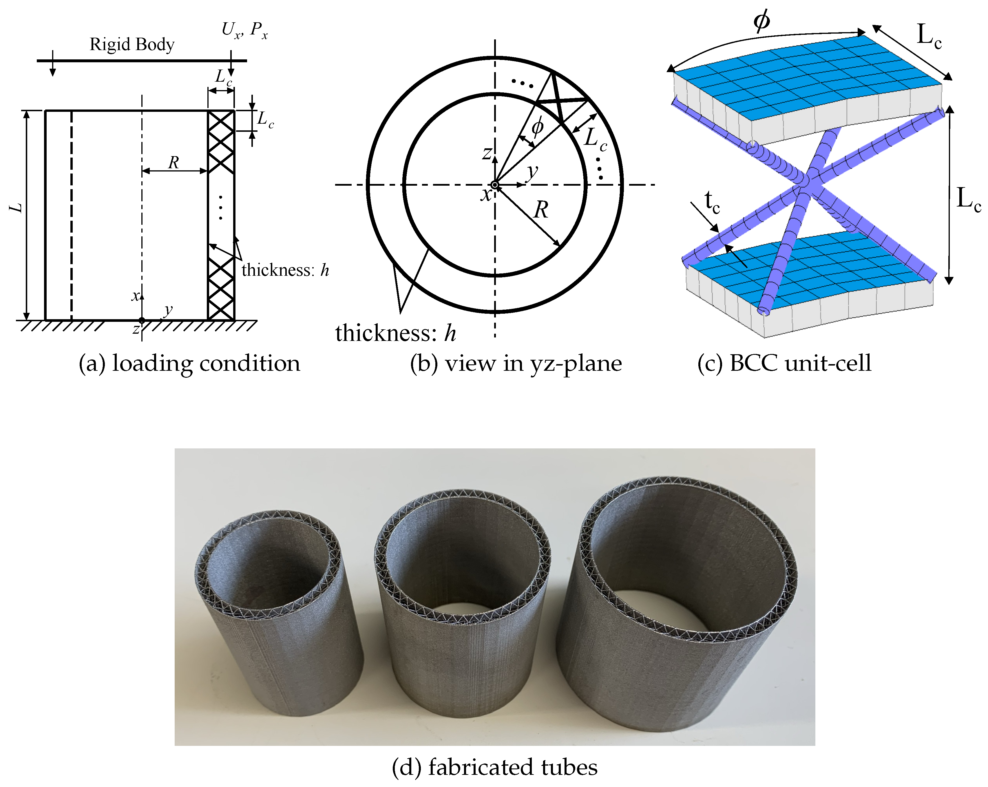
Figure 3.
Comparison of deformed shape of the lattice sandwich tubes with an inner radius R=30mm
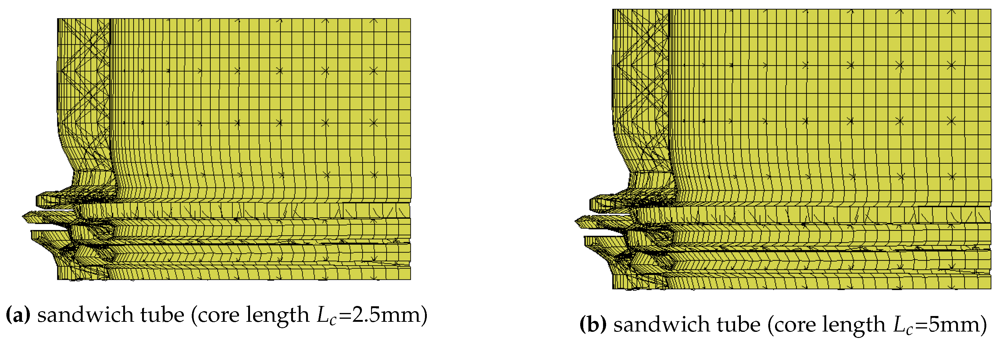
Figure 4.
Comparison of deformed shape of hollow tubes with an inner radius R=30mm
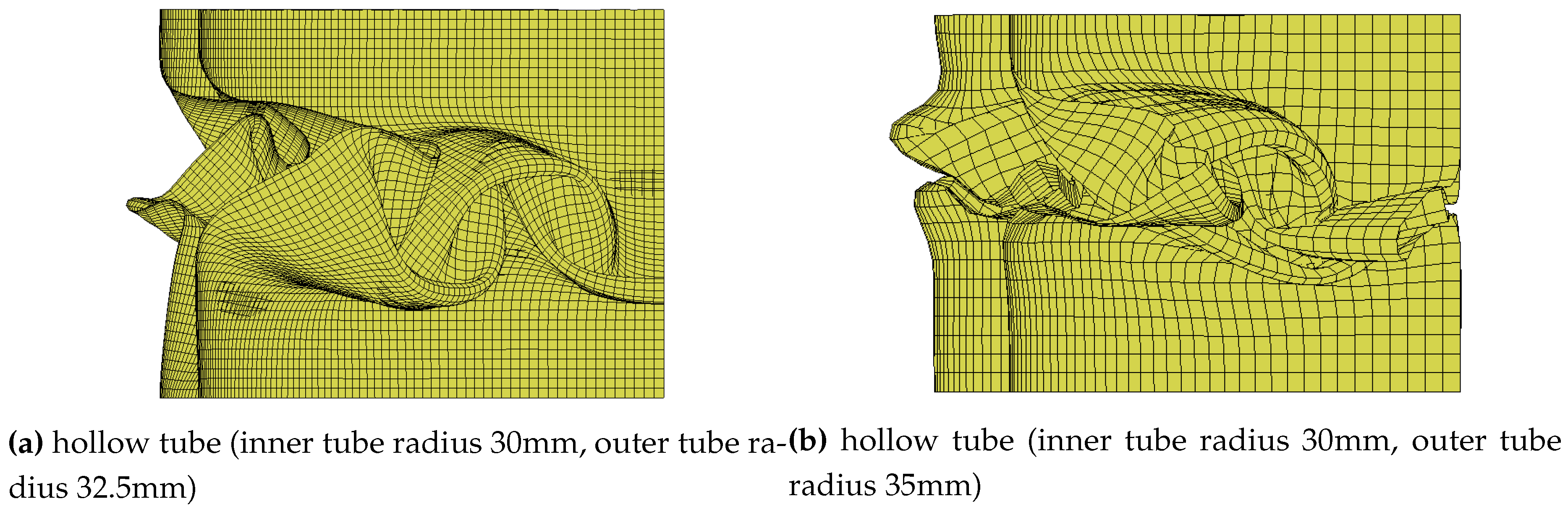
Figure 5.
Comparisons of the compressive load versus displacement curves and deformed shapes for lattice sandwich tubes based on the same strut diameter, =0.24mm
Figure 5.
Comparisons of the compressive load versus displacement curves and deformed shapes for lattice sandwich tubes based on the same strut diameter, =0.24mm
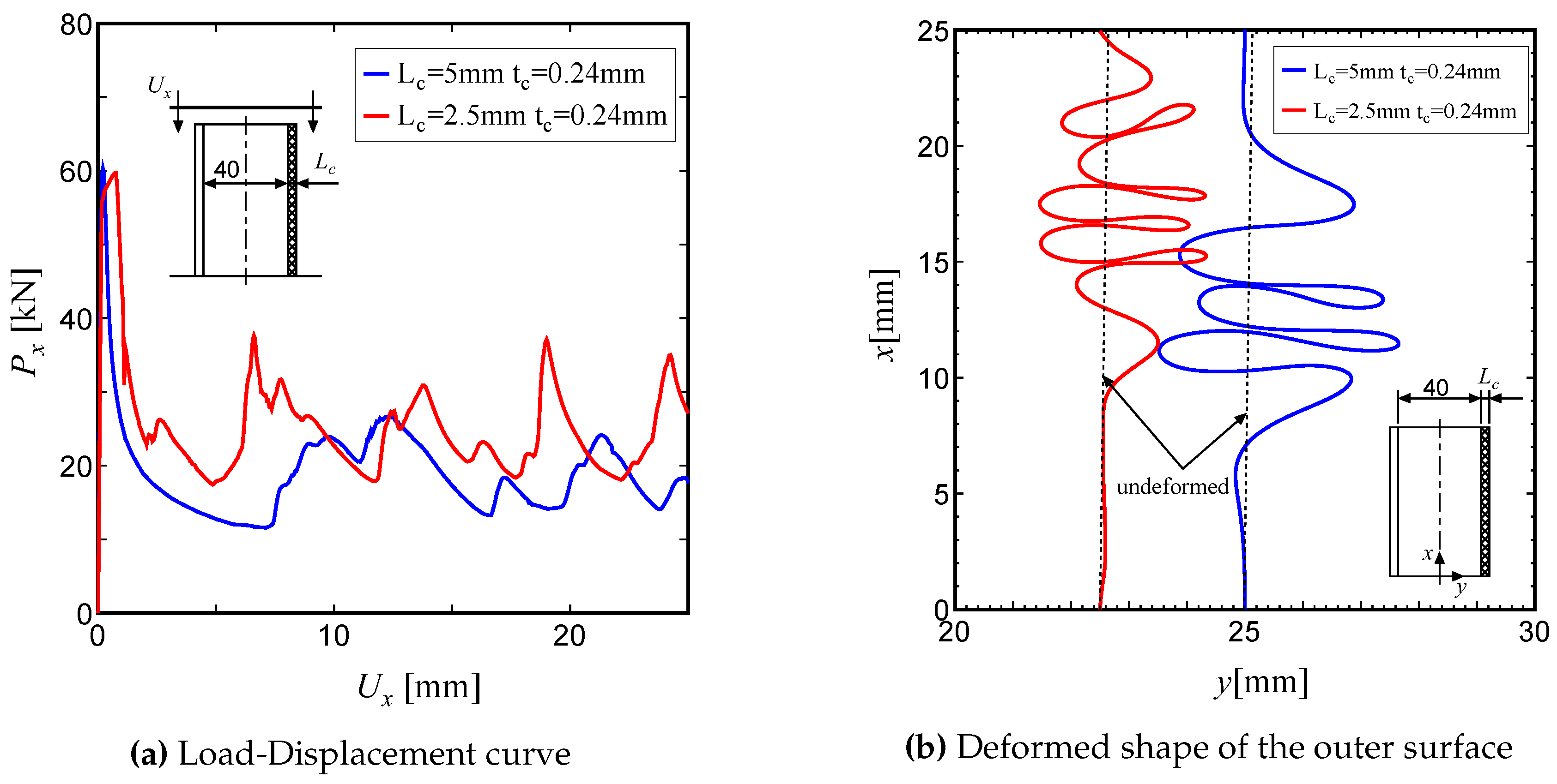
Figure 6.
Comparisons of the compressive load versus displacement curves and deformed shapes for lattice sandwich tubes based on the same core density
Figure 6.
Comparisons of the compressive load versus displacement curves and deformed shapes for lattice sandwich tubes based on the same core density
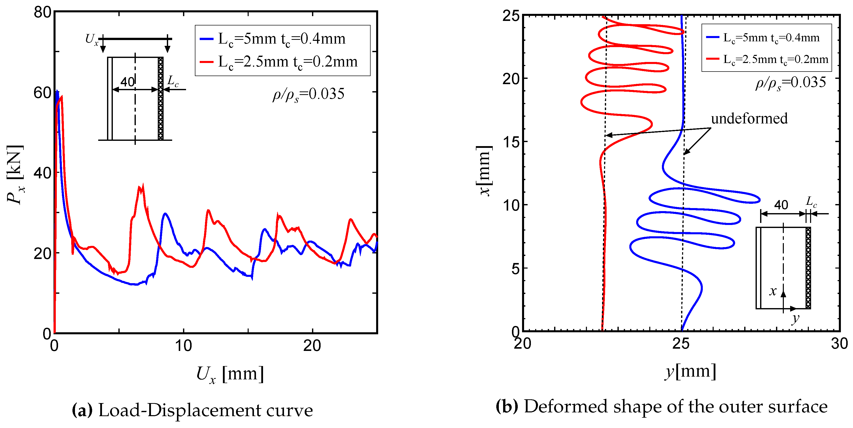
Figure 7.
Comparisons of load versus displacement curves for lattice sandwich tubes
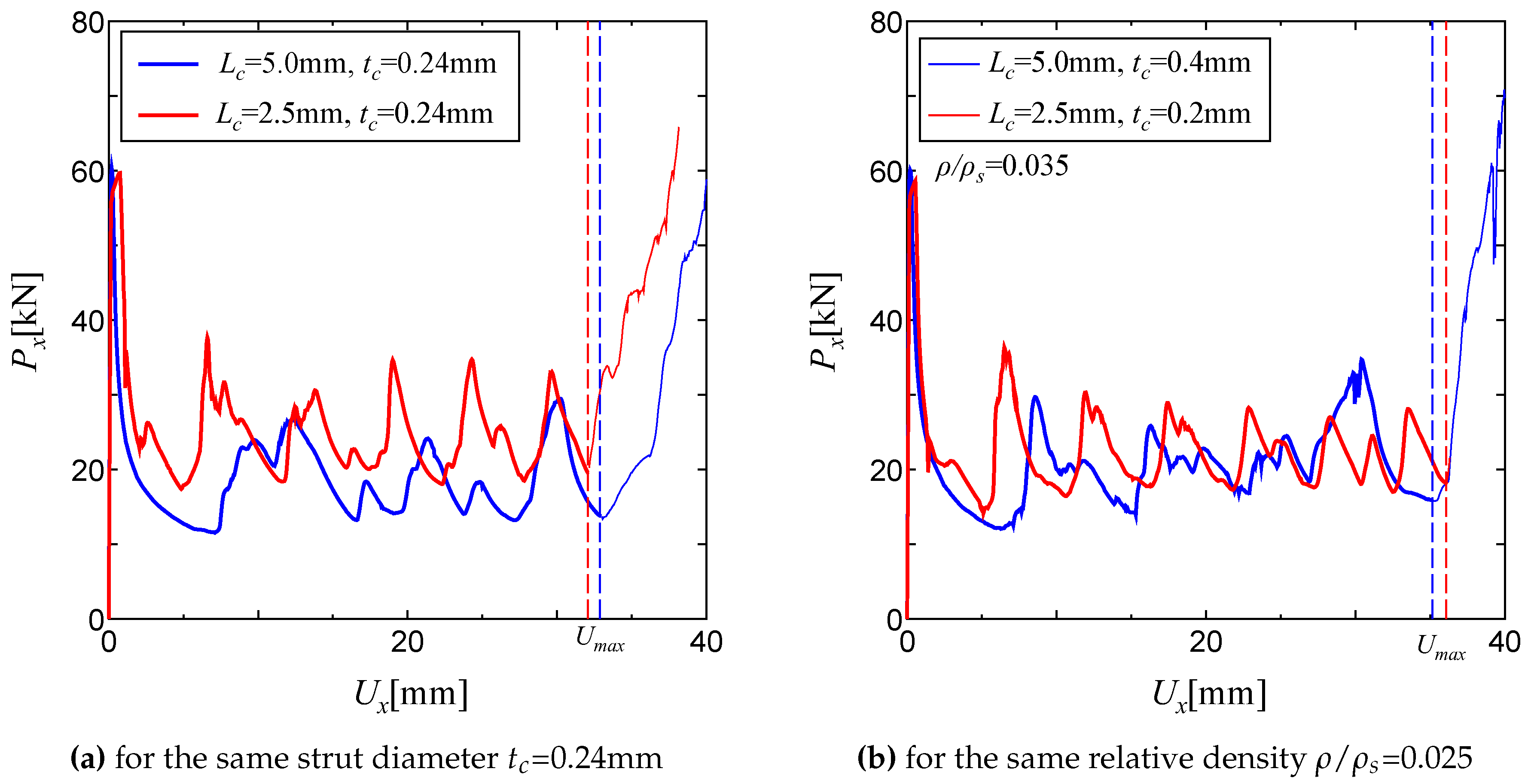
Figure 8.
Variations of the average stress as a function of relative thickness for lattice sandwich tubes with cell lengths =2.5mm and =5.0mm
Figure 8.
Variations of the average stress as a function of relative thickness for lattice sandwich tubes with cell lengths =2.5mm and =5.0mm
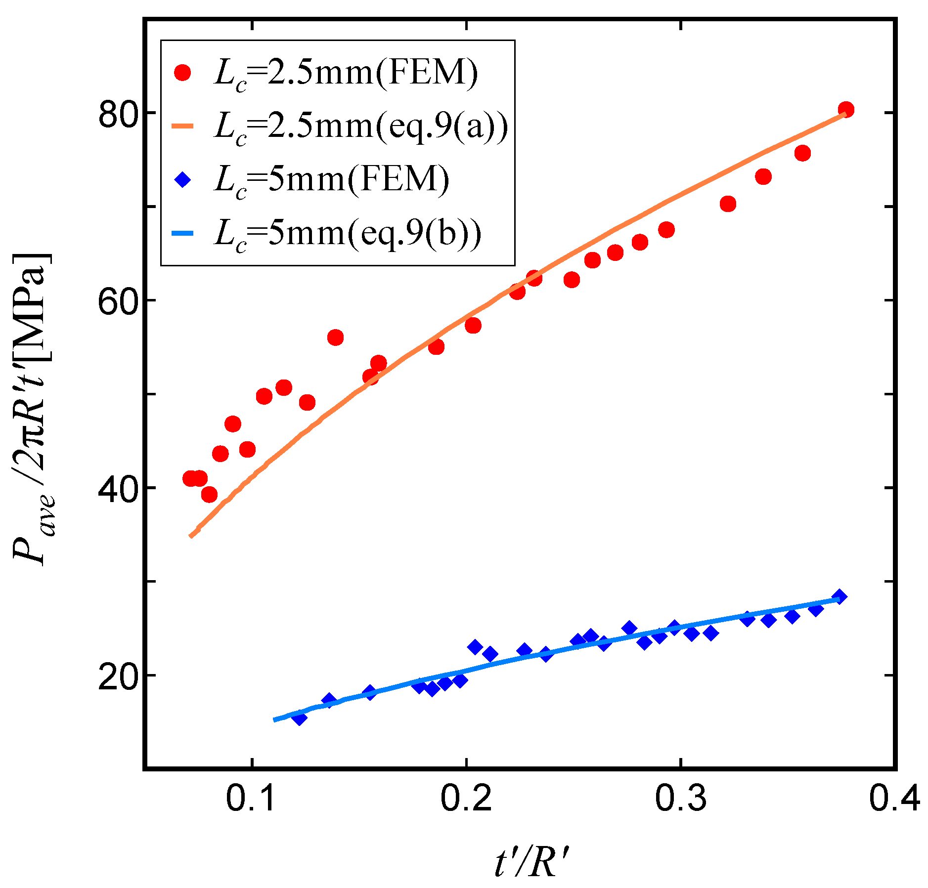
Figure 9.
Deformation mode map of lattice sandwich tubes with =5.0mm
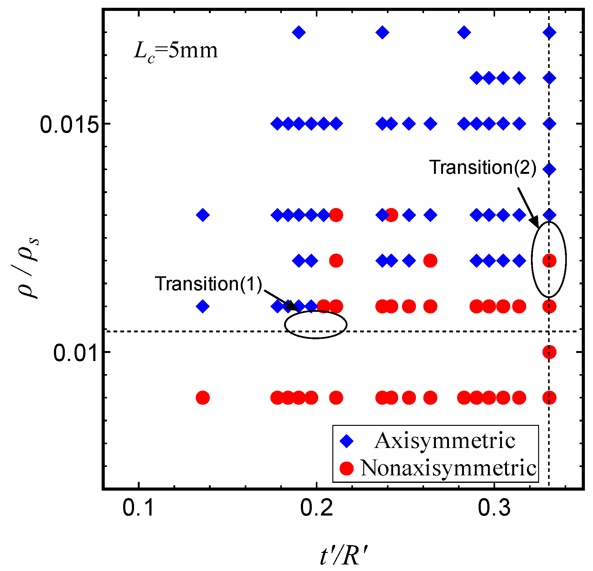
Figure 10.
Variation of the specific energy absorption (a) as function of the tube thickness-to-radius ratio and (b) as a function of relative density
Figure 10.
Variation of the specific energy absorption (a) as function of the tube thickness-to-radius ratio and (b) as a function of relative density
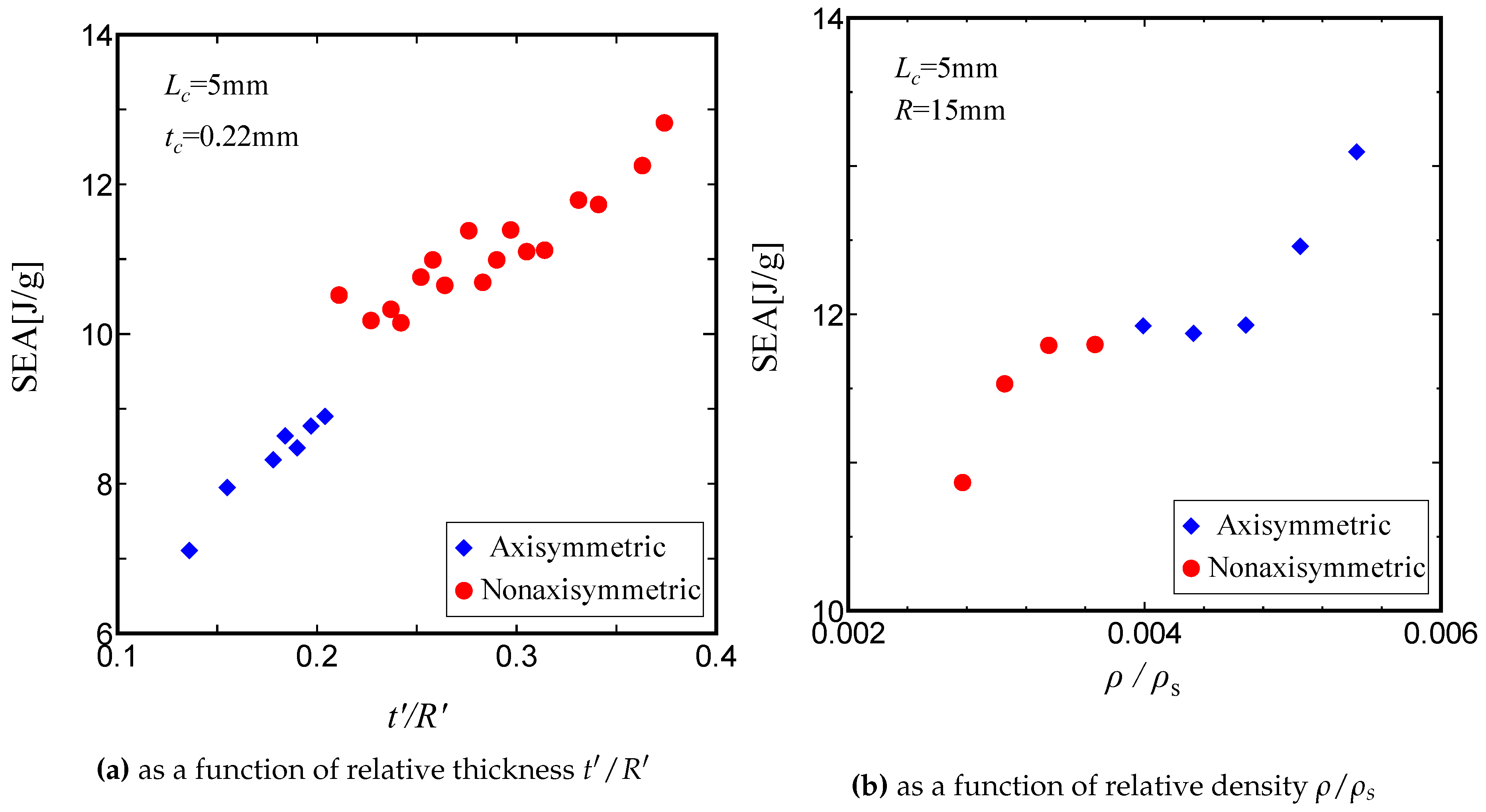
Figure 11.
Variation of the specific energy absorption of the lattice sandwich tube with relative density for a core length =2.5mm
Figure 11.
Variation of the specific energy absorption of the lattice sandwich tube with relative density for a core length =2.5mm
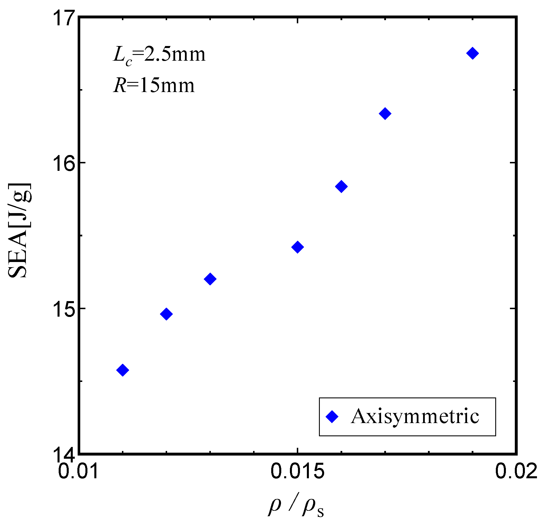
Figure 12.
Specimens following manufacture in the 3D metal printer

Figure 13.
A lattice tube positioned in the testing machine and a schematic of the compression test
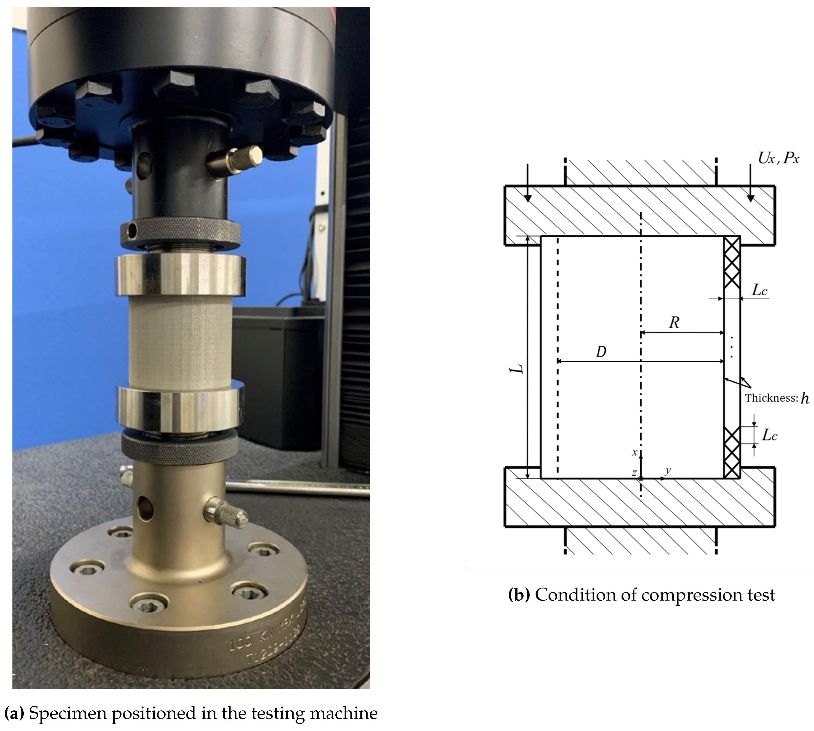
Figure 14.
Tensile stress-strain curve for SUS630
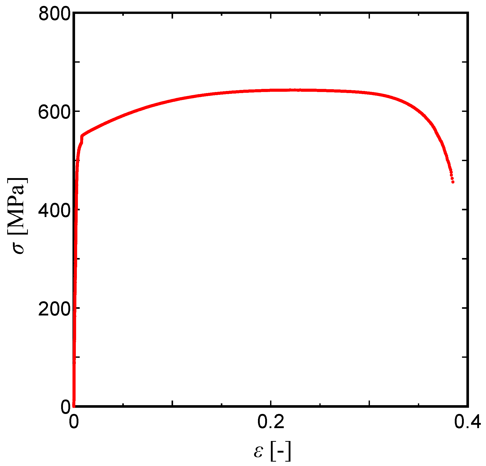
Figure 15.
Comparison of the compressive load-displacement curves for the thin-walled tubes(specimen shapes A,B,C) (a) experimental data and (b) FEM predictions
Figure 15.
Comparison of the compressive load-displacement curves for the thin-walled tubes(specimen shapes A,B,C) (a) experimental data and (b) FEM predictions
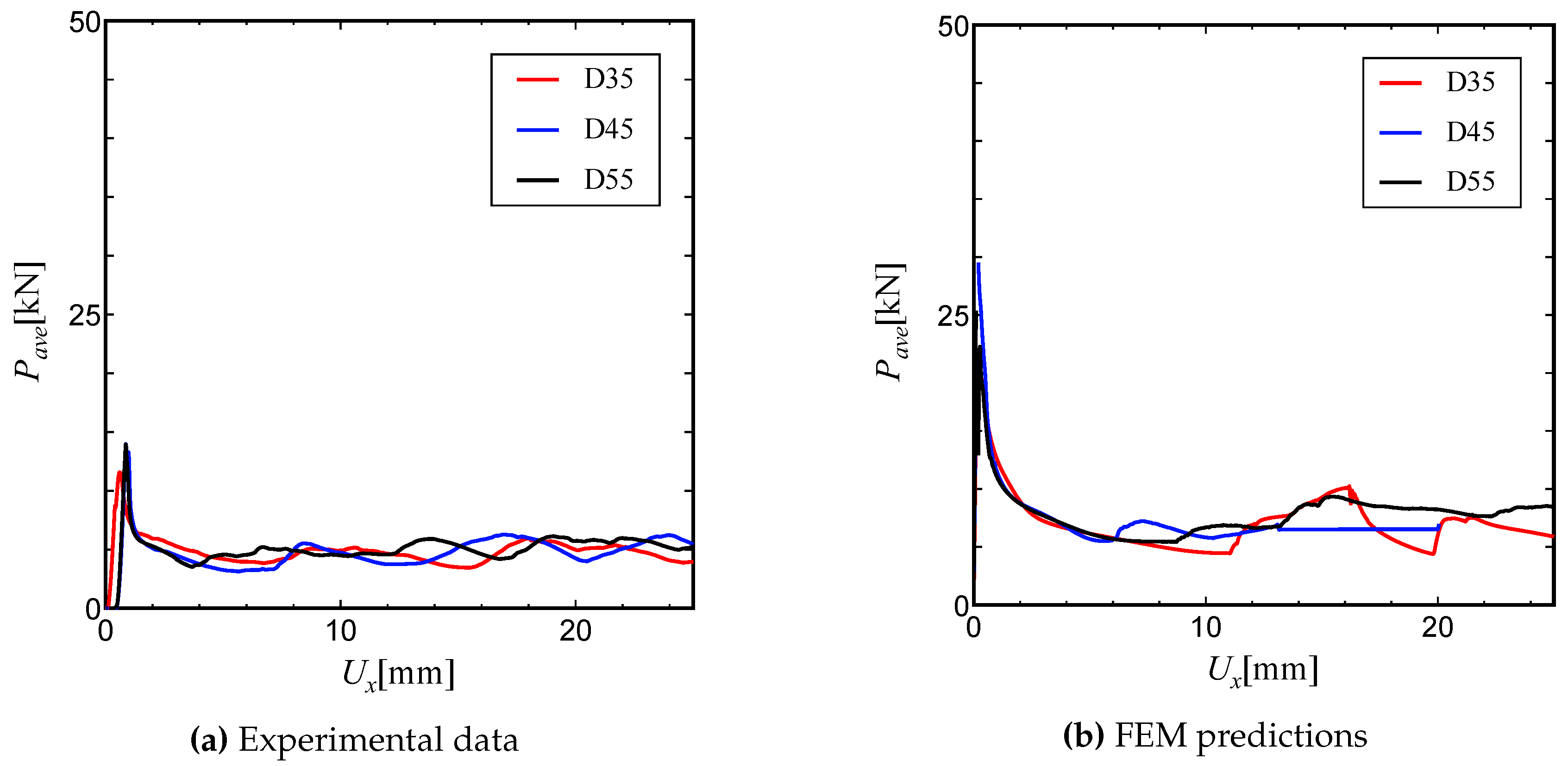
Figure 16.
Effect of boundary conditions for the nodes on both tube edges on the compressive load-displacement curve for the thin-walled tubes(specimen shape A)
Figure 16.
Effect of boundary conditions for the nodes on both tube edges on the compressive load-displacement curve for the thin-walled tubes(specimen shape A)
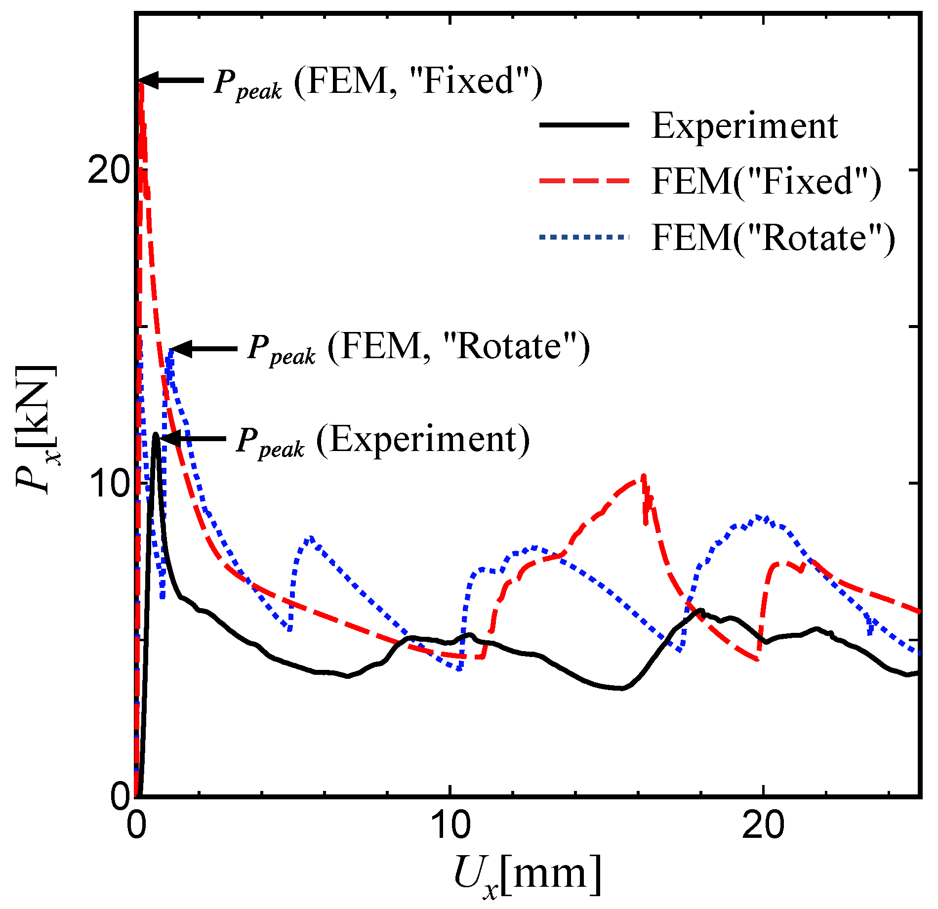
Figure 17.
Comparison of the experimental and numerical compressive load versus displacement curves for a lattice sandwich tube (D =30mm, Specimen shape D)
Figure 17.
Comparison of the experimental and numerical compressive load versus displacement curves for a lattice sandwich tube (D =30mm, Specimen shape D)
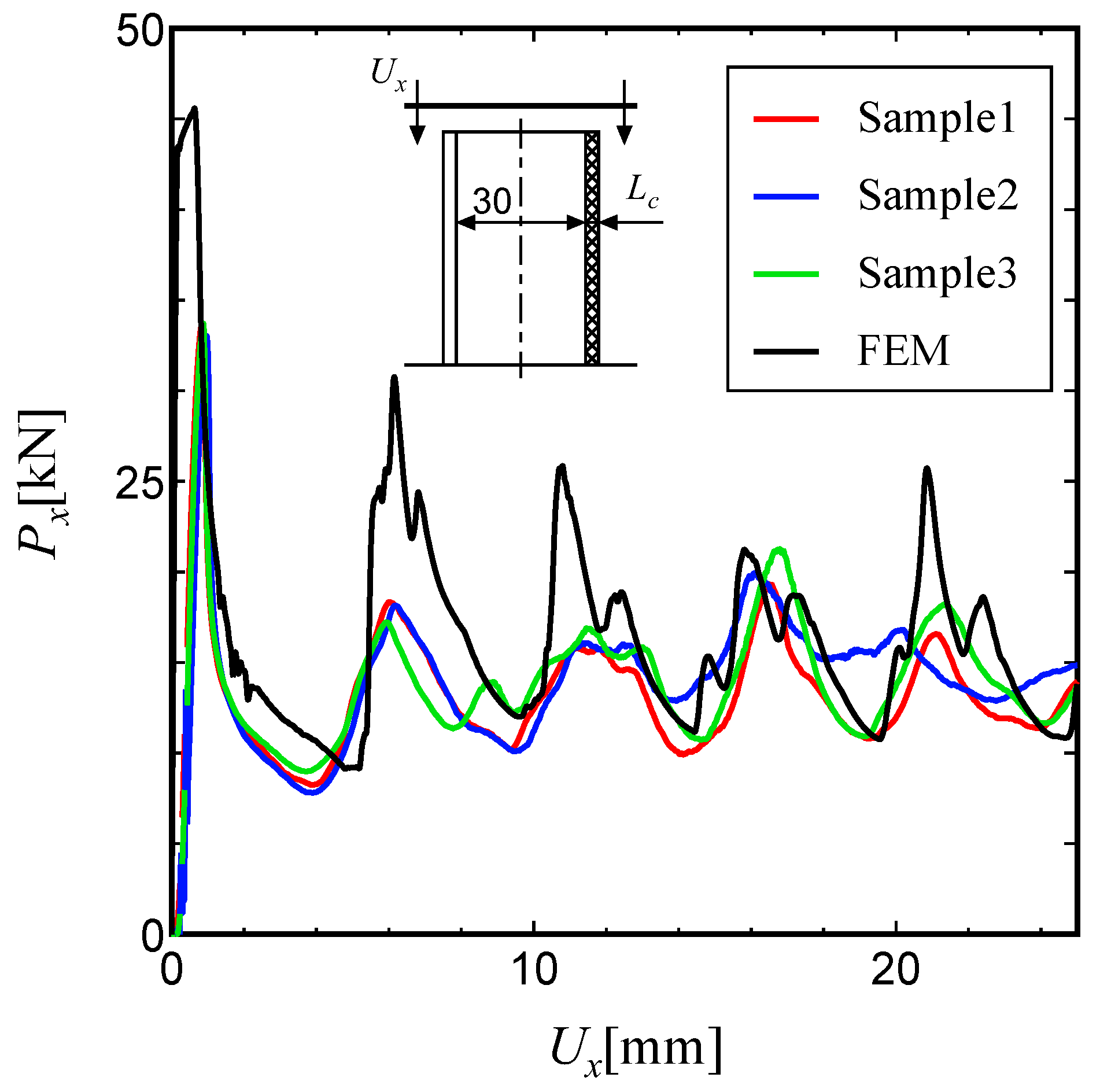
Figure 18.
Photographs showing the failure process in (a) a thin-walled tube with D=35mm and (b) a lattice-based sandwich tube with D=30mm
Figure 18.
Photographs showing the failure process in (a) a thin-walled tube with D=35mm and (b) a lattice-based sandwich tube with D=30mm
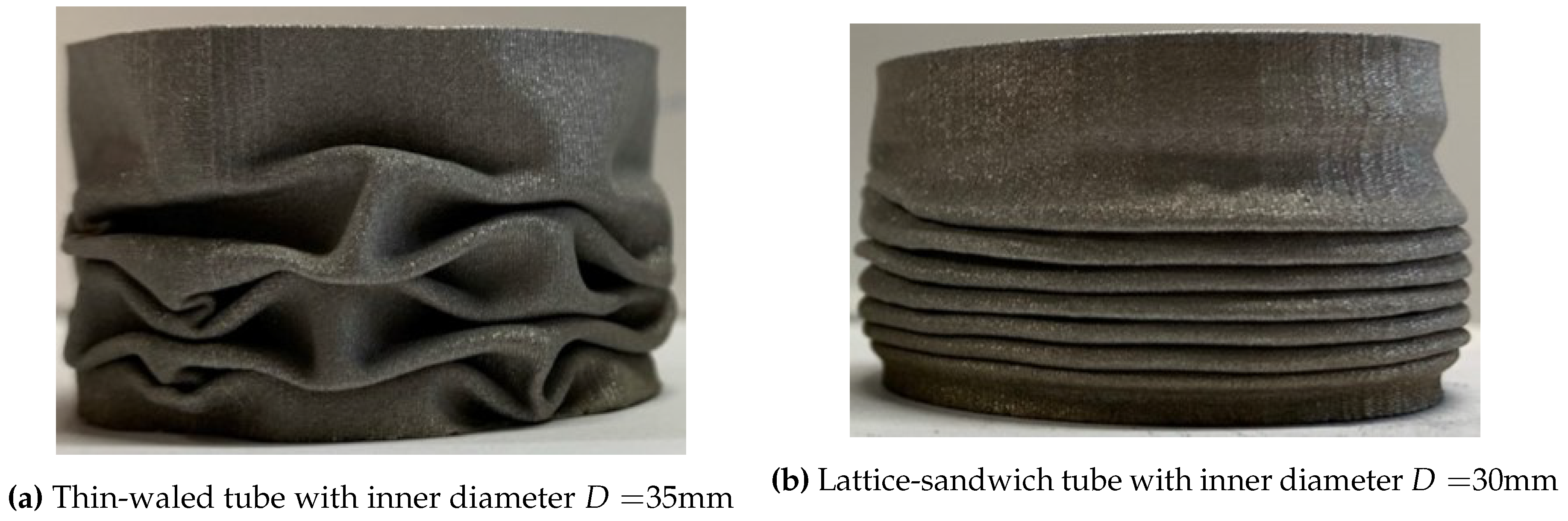
Figure 19.
Comparison of the experimental and predicted compressive load versus displacement curves for a lattice sandwich tube with D=40mm of compression test(Specimen shape E)
Figure 19.
Comparison of the experimental and predicted compressive load versus displacement curves for a lattice sandwich tube with D=40mm of compression test(Specimen shape E)

Figure 20.
Photograph showing the failure processes in (a) a thin-walled tube with D=45mm (Shape B) and (b) a lattice-based sandwich tube with D=40mm (Shape E)
Figure 20.
Photograph showing the failure processes in (a) a thin-walled tube with D=45mm (Shape B) and (b) a lattice-based sandwich tube with D=40mm (Shape E)
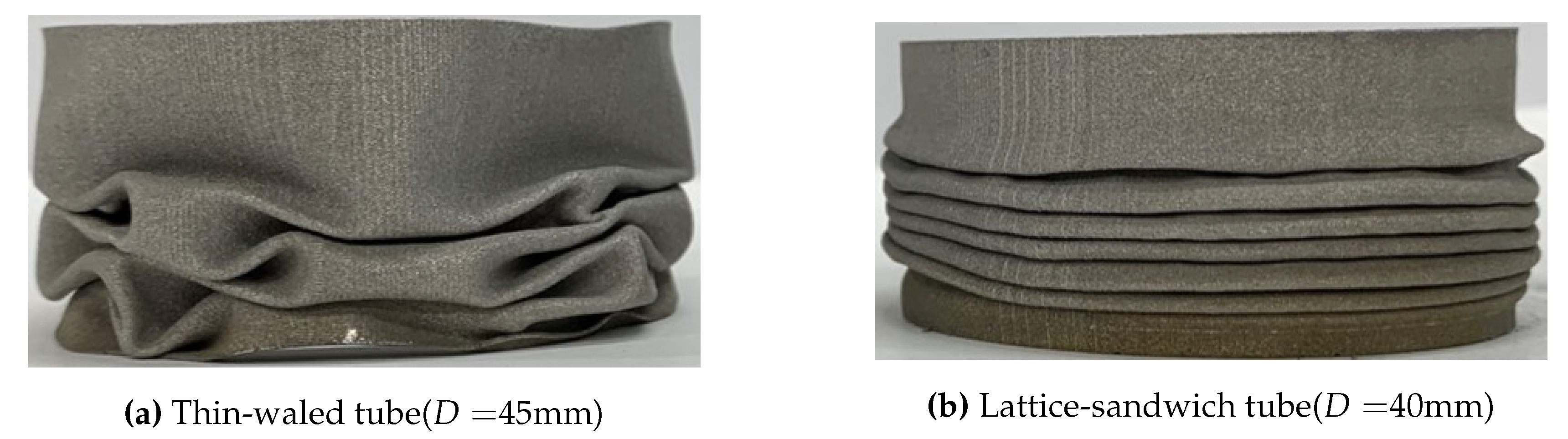
Figure 21.
Comparison of the experimental compressive load versus displacement curves for the lattice-based sandwich tube with D =50mm (Specimen shape F)
Figure 21.
Comparison of the experimental compressive load versus displacement curves for the lattice-based sandwich tube with D =50mm (Specimen shape F)
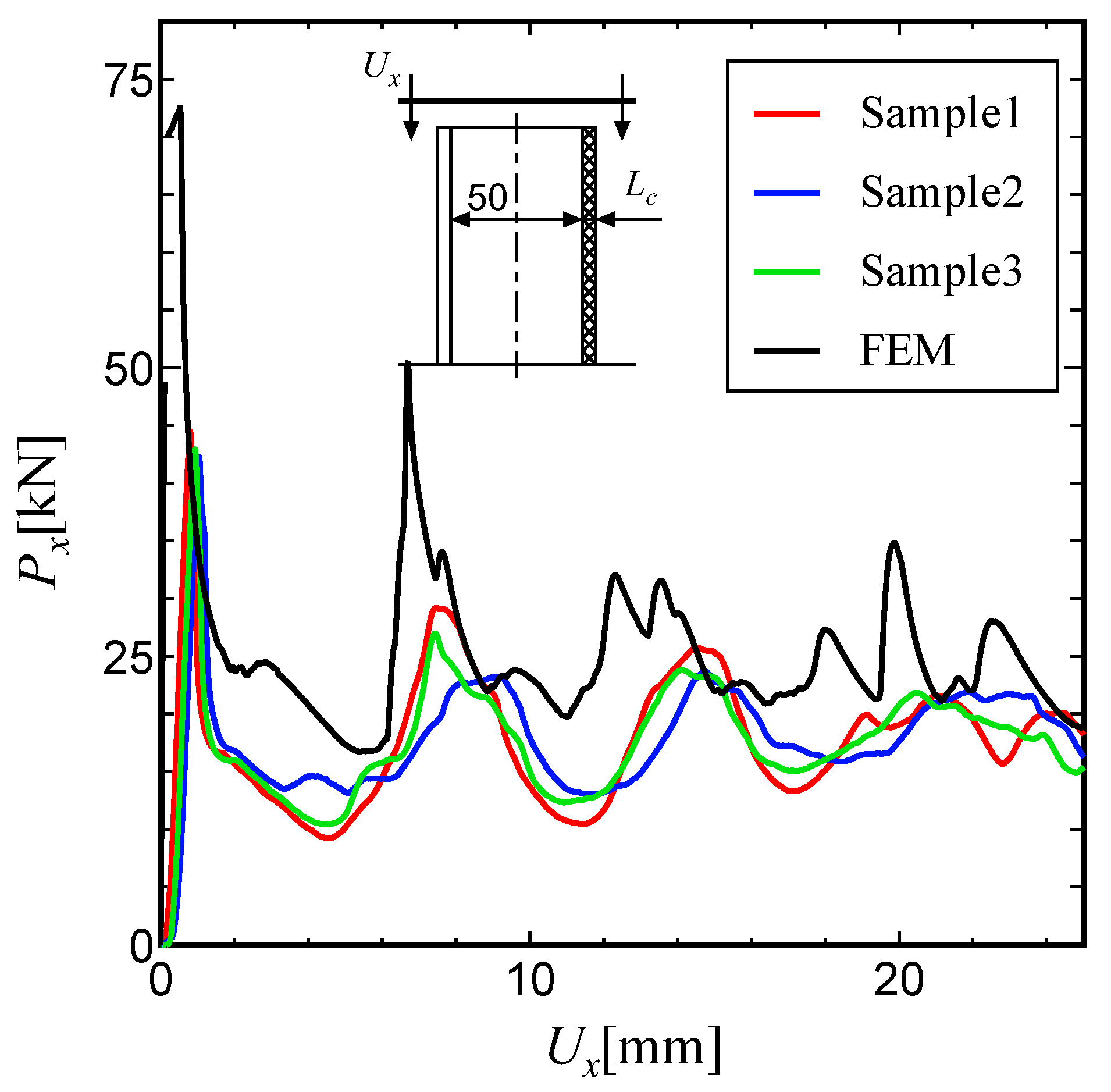
Figure 22.
Compressed Specimens of thin-walled tube (55mm) and lattice-sandwich tube (50mm)

Figure 23.
Relationship between the cylindrical wall thickness ratio and the average load
Disclaimer/Publisher’s Note: The statements, opinions and data contained in all publications are solely those of the individual author(s) and contributor(s) and not of MDPI and/or the editor(s). MDPI and/or the editor(s) disclaim responsibility for any injury to people or property resulting from any ideas, methods, instructions or products referred to in the content. |
© 2024 by the authors. Licensee MDPI, Basel, Switzerland. This article is an open access article distributed under the terms and conditions of the Creative Commons Attribution (CC BY) license (http://creativecommons.org/licenses/by/4.0/).
Copyright: This open access article is published under a Creative Commons CC BY 4.0 license, which permit the free download, distribution, and reuse, provided that the author and preprint are cited in any reuse.


