
Submitted:
16 December 2024
Posted:
17 December 2024
You are already at the latest version
Abstract
The growing amount of Renewable Energy Sources has led to the demand of innovative and high performing turbine designs. Due to the increase of computing resources over the last years, the numerical optimization with use of Evolutionary Algorithms (EAs) has become established. Nevertheless, EAs require a high number of expensive computational fluid dynamic (CFD) simulations and with an increasing number of design parameters, more computational resources are required. In this work, an adapted optimization algorithm is introduced. By employing an Artificial Intelligence (AI)-based design assistant, turbines with a similar flow field are clustered into groups and provide a dataset to train AI-models. These AI-models are able to predict the flow field’s clustering before a CFD simulation is performed. By analyzing the turbines properties inside the predicted clustering group, the turbine’s efficiency and cavitation volume are predicted. Turbines with properties below a certain threshold are not CFD simulated but estimated by the design assistant. By this procedure, currently more than 30% of the CFD simulations are avoided, significantly reducing computational costs and accelerating the overall optimization workflow.
Keywords:
Optimization
; Axial Turbine
; Clustering
; Auto Encoder
; Artificial Intelligence
; Evolutionary Algorithm
1. Introduction
The demand for Renewable Energy Sources (RES) has drastically grown in recent few years to reduce the use of conventional energy resources (such as fossil fuels) for power generation. In 2023, renewable energies have sourced almost one-seventh of the world’s primary energy. Additionally, until the end of 2050 up to 80% of the energy is expected to be produced by RES in the European Union. Hydropower accounts for almost 47% of all renewable energies produced in 2023 [1]. The contributions of other RES such as wind and solar have also grown. However, such undispatchable RES threaten the grid stability. Hydropower is capable to play a key role, not only in providing the emmission-free RES, but also in regulating and balancing the grid in both short and long terms [2]. These grid requirements demand durable, flexible and innovative turbine designs.
The increase in computing resources over the last few years provides the opportunity to design hydraulic machinery in an automated manner [3,4]. Besides the fluid mechanical properties, a hydraulic machine has to deal with unsteady mechanical loads leading to vibrations. In that sense, it is beneficial to optimize the machines simultaneously for fluid and structure mechanics [5,6]. These optimization tasks are computationally expensive and challenging due to the high number of time-consuming simulations required. The computational burden of the optimization task are generally non-linear with each added design degree of freedom (DOF) [7,8,9]. Each added DOF contributes in characterizing the "dimensionality" of the optimization task, hence becomes more and more resource-intensive. It is also known that Evolutionary Algorithm (EAs) need many evaluations of the problem to be optimized. In addition, many of the evaluations are only used during the ongoing optimization. In that sense, it is not always necessary to have an exact fitness value, because the optimizer decides depending on tendencies, better or not, and not on differences [10,11].
Recent developments in the computational methods as well as advancements in the hardware technologies have led to a drastic reduction of computational costs. As a consequence, optimizations based on EA generate much larger databases with an increased number of DOFs. This abundant data availability has enabled the integration of Artificial Intelligence (AI) into engineering discipline. Recently, this integration has rapidly accelerated in the field of fluid dynamics and design optimization, with numerous articles demonstrating the potential of Machine Learning (ML) in fluid dynamics [12,13,14].
An optimization task is complex and often involves a significant amount of high-dimensional data. ML offers effective approaches to address the "curse of dimensionality". Several ML techniques have demonstrated excellent performance in dimensionality reduction. Popular deep learning techniques include Deep Convolutional Networks (DCN) [15,16,17,18], Autoencoder (AE) [19,20,21,22,23,24], Generative Adversarial Network (GAN) [25,26,27], and Long Short Term Memory (LSTM) [20,28,29,30]. Among these, AE technology has shown exceptional results in the past case studies. Some past success stories are presented in [31,32]. This method extracts the essential building block information and projects it into an optimal low-dimensional space, known as latent space. It preserves crucial information, enabling reconstruction of the original data.
Following dimensionality reduction techniques, the clusters based on similar traits and behaviors are identified using clustering methods, also termed as community detection. In general, the community detection methods are classified into two major classes: (1) deep learning methods and (2) traditional methods. The later methods capture the relationships in a shallow, easier-to-understand manner. These methods mostly employ the strategies based on statistical and/or mathematical functions. Some of such methods are random-walk based dynamical clustering [33,34], density-based algorithms [35] and probabilistic models based statistical inference methods [36]. In the former case, deep learning approaches are utilized for the higher order dimensionality reductions for the data, followed by some Euclidean based clustering methods such as k-means clustering. Spectral Clustering has gained significant traction in recent years due to its versatility and effectiveness across various fields, including engineering, statistics, and natural sciences. Unlike traditional clustering algorithms, Spectral Clustering leverages the eigenvalues and eigenvectors of a similarity matrix derived from the data, allowing it to capture complex structures and relationships within data. The algorithm’s ability to handle non-convex clusters and its robustness against noise make it easier to implement and operate compared to other clustering techniques. Its applications extend to areas like text clustering, recommendation systems and traffic analysis, showcasing its broad utility and addressing diverse challenges in ML [37,38,39].
Building upon these advancements, this work targets the prediction of fitness values within the optimization of an axial turbine with a two-step fitness evaluation based on ML. In the first step, an AE is used to get the reduced dimensionality flow field. In the second step, clustering the flow fields using Spectral Clustering based again on the dimensionality reduced flow fields. This approach has been integrated into the in-house design system Design Tool Object-Oriented (dtOO) [3].
The main contributions of the presented work are as follows:
- Advanced pre-processing of the flow field and pressure data across the turbine blade.
- Encoding the processed data into the latent vector representation.
- Clustering the latent represented data into different clusters using Spectral Clustering.
- Evaluation of the fitness values of the turbines based on advanced clustering of the data.
- Integrating the approach to the in-house design system
The paper is structured as follows: Section 2 deals with the background information including details of dtOO, Non-Dominated Sorting Genetic Algorithm II (NSGA-II) and Spectral Clustering. In Section 3, the details about the problem definition and how AI is implemented to modify the workflow in dtOO are given. Results of the current study are presented in the Section 4. Discussions and concluding remarks are given in the Section 5.
2. Background
In this section, a comprehensive overview of the key components and methodologies underpinning the research is provided. The in-house dtOO framework [3] is described in detail, including its dependencies and code structure, which form the foundation of the optimization process. Additionally, the geometrical definition of the axial turbine is explained, which gives a clear picture about the design space being explored. A brief introduction of the optimization algorithm employed is provided, highlighting its role in navigating the complex design landscape. Finally, the clustering mechanism is discussed as a vital element in analysing and categorizing design variants.
2.1. Design Framework dtOO
The package dtOO was developed to have a framework that is free of license costs, flexible as well as extendable and that is able to deal with hydraulic machines. Figure 1 presents an overview of dtOO including its main dependencies, provided packages and additional implementation details. Main dependencies in dtOO are listed with a leading filled square symbol including their main functions within <>-symbols.
The packages, shown as rectangles, dtOOPythonSWIG, dtOOPythonApp and pyDtOO are responsible for interfacing Python, providing application builder algorithms and support evaluation of Open Field Operation And Manipulation (OpenFOAM) [40], respectively. If additional Computational Solid Mechanics (CSM) simulations are performed, CalculiX [41] provides the von Mises stress field. Additional dependencies that occur due to the executed Python script are given with an empty leading square symbol. Within the Figure, the island model [42,43] and the distribution to the nodes is schematically shown, too. The freely-shaped islands optimize the problem using an EA. During the optimization of one generation, there is no communication to the other islands; only after a predefined number of generations migration occurs. In order to have an asynchronous migration, migrants are stored in a migration database. The islands are able to send and receive candidates from the database whenever it is necessary. The second database is connected to each island and stores all evaluated candidates. This enables post-processing as well as migration techniques that also pick from that database and not only from the current existing generation.
The fat gray arrows represent the delegation of the simulation to a loadBalancer object. Due to the unequal duration of a simulation and, additionally, to multiple simulations per candidate evaluation, the loadBalancer distributes the jobs to the nodes. The input from the islands is processed in a first-in-first-out principle.
The dtOO framework is designed in an object-oriented way consisting of main classes that are shown on the right bottom part of Figure 1. Instances of each class except baseContainer are collected in Standard Template Library (STL)-like containers. All elements can be accessed either with a label or by its container’s index. The baseContainer is different, because it collects different classes, e.g. two and three dimensional vectors as well as points or transformers. The Figure lists besides the class names as well as their main purpose and responsibility. Besides the object-oriented structure, also instances of dtPlugin are able to extend the framework. It is easy to write a shared-object library with its desired user-intended extension code and load the library within the framework. This prevents recompilation of the framework.
2.2. Geometrical Setup of Axial Turbine
Figure 2 shows the runner of the test case. The three dimensional shape of the hydraulic machine is parameterized in dtOO using the Python interface dtOOPythonSWIG and the dtOOPythonApp builder algorithm library. The sketch I gives the definition of the meanline including its DOFs. It is defined in a two dimensional frame of reference in such a way that x and y correspond to and m, respectively. The coordinates and m are, namely, the circumferential and meridional direction. In the second sketch II the thickness distribution is visualized. The function is defined as a B-Spline curve of second order with five control points. In order to have smooth transitions at the leading edge of the blade, only a reduced number of control points’ coordinates are free to move. Combining the meanline and the thickness distribution results in the blade cut shown in sketch III. It is still represented in its two dimensional frame of reference. All two dimensional blade cuts are combined in a B-Spline surface by adding a constant spanwise coordinate s. The resulting surface is then defined in -m-s coordinates. The last step is to map each point of the blade to its corresponding position in the three dimensional channel. The final geometry of the blade is not directly constructed. It is created on demand for each point that is necessary during any procedure in the framework. It is clear that this costs performance, but prevents the algorithm from failing due to inaccuracies.
2.3. Optimization Algorithm
Described as "A fast and elitist multi-objective genetic algorithm" [44], the NSGA-II is designed to efficiently solve multi-objective optimization problems. The algorithm employs an iterative process to evolve a population of solutions, thereby demonstrating its elitism through the maintenance of high-quality solutions while promoting diversity among the solutions. In this application, NSGA-II is integrated into dtOO using the open-source PyGMO library [45]. The process begins with a population derived from Latin Hypercube Sampling (LHS), refined through k-means clustering to balance diversity and homogeneity. The algorithm sorts the populations’ candidates’ based on their fitness or, more precisely, based on the dominance of two individuals. A candidate C dominats D if C’s objectives are better or equal with at least one that is better than the objectives of D. In that sense, the solutions are ranked into Pareto fronts based on this rule. Within each front, a crowding distance metric ensures diversity by favoring isolated solutions. Genetic operators, including selection, crossover, and mutation, are applied to generate new populations, balancing exploration and exploitation.
2.4. Feature Extraction with AE
An AE is a type of unsupervised learning in ML paradigm, in which the input and output to the network are similar, with a low-dimensional bottleneck, also called latent space. Generally, it consists of two parts, an encoder and a decoder. An encoder represents the high-dimensional input F into a lower-dimensional latent data z. The decoder attempts to reconstruct similar to input from this lower-dimensional latent data z. Thus, an AE learns a compact representation of high-dimensional data. Training an AE involves the minimization of the error between original input F and reconstructed input . As a consequence, the hidden layers try to learn good compressed representations of the input. In this learning approach, the AE learns to capture most salient features of the input data F, making them useful for generating lower-dimensional embeddings for subsequent machine learning algorithms [32].
2.5. Spectral Clustering
Clustering refers to the grouping of the individuals on the basis of mutual similarities. Spectral methods refer to a set of algorithms that utilizes the eigenvalues and eigenvectors of specifically designed matrices constructed from data. Due to its simplicity and effectiveness, Spectral Clustering is beneficial for many different applications. It is most often used with other sophisticated algorithms to enhance performance [46]. Spectral Clustering methods strongly rely on the graph networks [47]. Consider be the set of patterns. A complete, weighted undirected graph with the set of nodes corresponding to n patterns and edges defined through the adjacency (affinity) matrix W with representing the weight of the edge between node i and node j. If the edges are undirected, then the matrix is symmetric and fulfills . The mathematical adjacency relation between two patterns is given as:
The function
gives the similarity between patterns. The function b is the dissimilarity between patterns and controls the decay rate of h. The degree matrix D is defined as a diagonal matrix whose elements are the degrees of the nodes of G:
Within this, the clustering problem can be seen as the graph cut problem [48] where the aim is to separate a set of nodes from the complementary set . This separation is crucial because it allows us to identify distinct groups within the data by minimizing the connections (or weights) between the nodes in set S and those in its complement . The objective of the graph cut problem is to find a division that results in the least total weight of edges connecting the two sets. Thus, this problem is formulated as an optimization problem, where the aim is to minimize the cut cost defined by the sum of weights of the edges that cross between two sets. This optimization framework provides a powerful method for identifying clusters within the data represented by the graph. This transition effectively connects the concept of complementary sets to the formulation of graph cut problems in clustering. Mathematically, the graph cut problem can be formulated as:
These cut optimization functions are very complex. They can be relaxed by using spectral concepts of graph analysis. These are given by the Laplacian matrix L and the normalized Laplacian matrix given as:
2.6. Gaussian Process Regression
Random variables that are described as a joint Gaussian distribution specify a Gaussian Process (GP) and can be used in regression. In this work, Gaussian Process Regression (GPR) is used to predict the fitness values of the axial turbines. In GPR, prior knowledge is supplemented by likelihood knowledge the training data with training output , to deliver predictions for unknown data points .
A GP is solely described by its mean (here set to zero) and the covariance function with by:
The covariance function describes the covariance between the outputs f, only dependent on the input data x. It characterizes the deviations in output space f depending upon the input data x. Therefore, it determines the characteristic of the possible regression functions for the process. Through element-wise computation of for each pair of data points the covariance matrix is computed. The prior distribution of the probability variables of the prediction data is normally distributed and given by:
Combining the training data with the prediction data gives
Conditioning this distribution on the (previously known) training data delivers the posterior distribution for the prediction data :
For more detailed information, it is referred to [51].
3. Problem’s Description and Workflow’s Modification
This section provides a detailed overview of the problem related to optimizing axial turbines, focusing on how the fitness value is defined and evaluated. Additionally, this section highlights the important changes made in the optimization workflow.
3.1. Axial Turbine
An axial turbine with four blades is chosen as a test case. The quarter section of the axial turbine is shown in Figure 2. The geometry consists of a runner channel with a blade as well as a hub and shroud with radius and , respectively. This test case is evaluated using three different load conditions: nominal, part and full load. The volume flow rates at part and full load are set to and times the discharge at nominal load, respectively.
3.2. Numerical Setup and Optimization Problem
The framework dtOO provides support for hybrid meshes. This means that the axial turbine is meshed with tetrahedrons, prisms, pyramids and hexahedrons. In order to have correct predictions of the pressure and shear forces on the blade as well as on hub and shroud, the candidates are meshed with a structured mesh block as well as prism layers, respectively. The former is necessary for correctly predicting the flow surrounding the blade and, additionally, remain flexibility due to filling up the remaining blade free channel with tetrahedrons. The latter remains the benefits of unstructured meshes as hub and shroud sections vary strongly during the optimization process. Computational Fluid Dynamics (CFD) simulations for the evaluations are performed with OpenFOAM using version . The rotational speed of the turbine is set to 72 and pressure at the outlet is set at 0 . The turbulence model is used in the performed CFD simulations. Inlet velocities and turbulence quantities are interpolated from an intake section to the actual inlet of the turbine to achieve real-life inflow conditions.
The fitness function for the axial turbine is a multi-dimensional function consisting of three values extracted from the CFD simulation. Each turbine is evaluated based on an averaged efficiency
and cavitation volume
as well as the deviation in head
for the nominal operating condition. The functions and are penalty functions. The fitness function
is an "averaged fitness" in all operating points except for head.
3.3. Modification of the Optimization Procedure
This work introduces an AI-based design assistant for the optimization of the problem. Simply put, the design assistant extracts the features of the problem’s flow fields, creates clusters and approximates their fitness values. Each flow field is divided into Flow Area (FAs) surrounding the blade. The results of each FA are then clustered. These clustering results form the Cluster-ID (CI) that describes the flow field of a candidate. Undesired flows are identifiable depending on their CI. To detect turbines with unwanted flow properties before simulation, a Neural Network (NN) is implemented for each FA. The NNs predict the CI based on the candidate’s DOFs. These NNs prevent turbines with unwanted flow fields beforehand, thereby avoiding time-consuming simulations. Each new candidate suggested by the optimization algorithm is then evaluated based on its cluster position to determine whether a simulation is necessary.
3.3.1. Flow Field Extraction
The flow field of a turbine is extracted at predefined coordinates relative to the turbine’s blade. Since the blade geometry of each turbine varies through the optimization process, the coordinates must depend on the blade geometry. They cannot remain fixed in space in order to ensure comparability between different turbine geometries. Therefore, the velocity and pressure data is extracted for each cell within the hexahedral boundary layer of the hybrid mesh. These cells maintain logically the same position in relation to the blade. As shown in Figure 3, the flow field around the blade is divided into eight FAs. This division enables the comparison of flow phenomena corresponding to specific blade regions, such as the leading edge, across different simulations. As a result eight distinct tensors with flow field information are obtained per simulation.
Pressure and velocity data is extracted for each coordinate in the hexahedral mesh area of the test case. Therefore, a four-dimensional tensor consisting of the extracted data and the three spatial coordinates is received. Since three different operating points are considered, one candidate evaluation contains three CFD simulations to receive its fitness values in the optimization process. To compare the flow fields, the three simulation results are combined by stacking up the tensors for each operating point in their last dimension. Due to that, turbines within the same cluster share similar flow fields in all three operating points. Before clustering, each tensor is converted into a low-dimensional space by a three-dimensional convolutional AE. Both the encoder and decoder use four layers as shown in Figure 4. The feature vector is received within the latent space of the AE. As each flow field is divided into eight FA, eight distinct feature vectors per turbine are obtained.
3.3.2. Clustering
One clustering task per FA is performed to compare different turbines regarding their flow in this FA. These tasks are conducted independently for each FAs. Consequently, eight different clustering tasks have to be completed in total, Figure 5. Each turbine is assigned to one cluster per FA, resulting in a total of eight cluster assignments per turbine. For each FA, a turbine receives a Cluster-Number (CN) within the range k] with the Amount of Clusters (k) being the maximum number of clusters in this FA. These eight CNs collectively form the CI, which uniquely identifies the turbine’s flow group assignments across all FAs. The flow fields of two turbines are considered similar if their CNs are identical across all eight FAs, resulting in matching CIs. It is important to note, however, that turbines with the same CI do not necessarily have identical flow fields. Instead, their flow fields share common properties as determined by the clustering algorithm.
3.4. Investigation of Turbines that Share the Same CI
As mentioned earlier, turbines that have equal CIs also share a similar flow field. Investigating the properties of these turbines shows that they also share similar fitness values. An exact assignment of CI to fitness properties is not possible, but Figure 6 indicates that the CI is able to deliver an approximation. The presented result on the left side of Figure 6 is based on a dataset consisting of 500 turbines. The clustering algorithm’s behavior is affected by the freely determinable parameter k. A higher value of k enables the algorithm to distinguish more precisely between different flows. Generally, flow fields with the same CI share more similar fitness values. However, a higher k also leads to more CIs in the dataset, meaning fewer simulations share the same CI.
To investigate the influence of k on the clustering quality, the similarity of flow fields sharing the same CI are compared for different values of k. To define a criterion, the pressure values on the blade generated by the flow are extracted. All pressure surfaces of candidates that have equal CIs are superposed, see the left side of Figure 7. Subsequently, for each CI, the envelope of these pressure surfaces is determined by computing the upper and lower limits of these surfaces. The mean thickness of this envelope determines the quality of the clustering. A slimmer envelope indicates more similar flow fields sharing the same CI. An example for a thickness distribution of an envelope is shown on the right side of Figure 7. Similarly, the average of the thicknesses of all the CIs’ envelopes is an indication of the quality of a specific choice of k.
As shown on the right side of Figure 6, the mean thickness decreases as k increases. It is again explained that more available clusters will reduce the number of candidates in each cluster. On the one hand, if k is too high, each cluster contains only one candidate. On the other hand, if k is too low, all candidates are within the same cluster. Therefore, it is important to find a trade-off. The authors believe that the area between k = 15 k = 20, 20, surrounding the saturation point shown on the right in Figure 6, providesanoptimaltrade-off.
3.5. Mapping of CIs Using a NN
To predict the turbine’s CI prior to performing the CFD simulation, a multi-class prediction NN is implemented. It contains one NN for each FA. The inputs of the NN are the DOFs that vary the parameter of the geometry. The network is then trained to predict the CI. Figure 8 shows two NN in the center part. Each NN contains two hidden layers with 64 and 54 neurons, respectively. The first and last layer are defined by the number of DOFs and k, respectively. The NN is updated during the optimization run so that new simulated turbines are added to the training dataset. The NNs are used to predict the CI immediately after the optimization algorithm suggests a new candidate. The predicted CI provides an approximation of the flow field for the turbine that has not yet been simulated. This enables the evaluation of the turbine’s properties without performing a CFD simulation.
3.6. Integration of CIs into Optimization Process
The results in Section 3.4 show that the CI, in combination with the trained NNs, provides an approximation of the turbine’s fitness values. For every new candidate, suggested by the optimization algorithm, the NN first predicts the CI. This is visualized in Figure 8 with the black lines connecting the input parameters and the NNs on the left side. The fitness approximation is initially calculated as the mean fitness value of all candidates with equal CIs. For CIs with mean fitness values above a certain threshold, the candidate’s fitness value is not simulated but estimated by the design assistant. Figure 9 illustrates the structure of the design assistant.
Before a longer optimization with the adapted optimization algorithm is run, the design assistant’s performance depending on k is investigated. Two different threshold-based approaches are used for deciding whether to simulate the turbine or not (decision "Simulate Turbine?" in Figure 9). In the first approach, a candidate is simulated if the approximated is above the 50% quantile of the initial training data set for the clustering procedure. If not, the candidate’s fitness values are approximated by the design assistant. This approach is used for the investigation of the design assistant’s performance. In the second approach the threshold is based on the candidates during the optimization and, in that sense, dynamically adjusted during the run. The weighted sum for all operating points is used here. All turbines with a predicted fitness value above the 40% quantile of the last 250 turbines are estimated by the design assistant. This approach is used, during the longer optimization run, to adapt to the latest optimized turbines’ fitness values. (Note: ).
To investigate the design assistant’s prediction performance before running a longer optimization, two different approaches for the fitness prediction are compared. The first approach estimates the fitness values by calculating the mean fitness values of the candidates with equal CI. In the second approach, the fitness estimation is extended by a GPR using all turbines of the same CI as training data. The turbine blade’s geometry DOFs serve as inputs for the GPR. Since, the number of turbines with equal CIs might be small and the number of DOFs is very high, a Principal Component Analysis (PCA) reduces the dimension of the DOFs. Within the GPR, a Radial Basis Function Kernel is used for the covariance functions. In both approaches, if the NN predicts a CI that has not occurred before, the candidate’s fitness is simulated.
4. Results
To investigate the design assistant’s prediction performance dependent on k, an optimization with the NSGA-II is used, applying an island model with ten islands. Within the first investigation, the influence of k = 16 k = 20 the results is investigated with a focus on the Spectral Clustering algorithm. The first 1000 candidates are simulated conventionally and used as initialization for the
adapted optimization as well as for the design assistant. The optimization of the next 1000 individuals
is performed with the adapted optimization algorithm. The prediction accuracy of the design assistant
is evaluated by resimulating the previously approximated candidates. Table 1 displays the deviations
for the fitness prediction depending on k and GPR. The GPR is only used, if at least two different
individuals share the same CI. Even with the integration of GPR, some fitness values are still predicted
by the CI’s mean fitness values if there is not more than one different turbine sharing that CI. The
overall best performance delivers k = 20 with use of GPR. This configuration is used for the longer
optimization run. Figure 10 shows the difference for the approximated and simulated fitness values
for k = 20 with and without the use of GPR.
Before the longer optimization starts, each of the design assistant’s AE is pretrained by the initialization dataset. After each tenth generation on the first island, the AEs are retrained by the updated database. The NNs for CI prediction are also retrained after every tenth generation on each island. The same initialization dataset is used as for the performance investigation. This time the dynamically adapted threshold for the simulation decision is used. Every CI with an expected fitness above the 40% quantile of the last 250 candidates is not simulated but estimated by the design assistant.
Each island runs its own computing process and therefore, each island runs its own design assitant’s Python object. The optimization process runs asynchronous on each island. As a result, the retraining of the NNs and the threshold adjustment run asynchronously for each island, even if the objects of the design assistant share the same database. Figure 11 shows the resimulated fitness values of the previously estimated turbines during the optimization run. The turbines’ fitness values are sorted by their chronological occurrence. The green line marks the 40% quantile threshold. Target of the design assistant is to keep the resimulated turbines’ fitness above the threshold line. Mean and standard deviation of the complete database’s fitness values are shown as black and red lines.
Figure 12a illustrates the current ratio of the turbines estimated by the design assistant to the turbines suggested by NSGA-II along the optimization process. With the ongoing optimization, the design assistant’s database contains more turbines. Therefore, more CIs are already known by the design assistant. As a consequence, fewer CIs predicted by the NNs are unknown and must therefore, be simulated using CFD and the ratio of estimated turbines increases.
The prediction deviation, both for fitness and for the cavitation volume , is illustrated by Figure 12b. While the prediction deviation initially increases, a decrease is noticeable after 5000 candidates, especially for the cavitation volume.
Figure 12c shows the maximum amount of turbines sharing the same CI along the course of the optimization. In all three Figures, the x-axis displays the course of the optimization for the turbines proposed by the NSGA-II.
The optimization’s Pareto front is presented in Figure 13. The dots mark the initialization dataset. The triangles mark the latest Pareto front of the optimization adjusted by the design assistant. During optimization, turbines with high efficiency are found, while retaining a low cavitation volume. Since the head was a constraint of the optimization, the head deviation from target is represented by the color bar.
5. Discussion
This work presents an innovative approach to evaluate axial turbine fitness properties without relying solely on computationally expensive CFD simulation. By employing a clustering-based design assistant, the method significantly reduces the computational burden typically associated with turbine design optimization. The clustering-based approach leverages AE followed by Spectral Clustering techniques to analyze and group similar flow field patterns around axial turbines. This method allows for rapid assessment of turbine performance characteristics, offering a more efficient alternative to traditional CFD simulations. In combination with NSGA-II, an adapted optimization algorithm is introduced. This hybrid approach integrates the clustering-based fitness evaluation with the multi-objective optimization capability of NSGA-II, enabling a more efficient exploration of the design space. The optimization results provide the following insights:
- The design assistant predicts turbines’ fitness values with a reasonable accuracy and can group turbines of similar flows.
- Even with a dataset of fewer than 1000 turbines, the design assistant can identify similar flow fields and predict fitness values without performing a CFD simulation.
- The adapted algorithm can identify turbines with bad fitness values and avoid time-consuming simulations of those turbines. With ongoing optimization, the ratio of currently estimated individuals rises above 30%.
- During optimization 9000 individuals are evaluated. The adapted optimization algorithm estimates of these. Since the computational effort of training the AI-based design assistant is negligible, around of computational resources are saved by integrating the design assistant into the optimization process.
- The adapted optimization algorithm finds high efficiency and low cavitation individuals, that dominate the initialization individuals. An advancing Pareto front is created.
Particularly useful is the design assistant’s ability to bypass CFD simulations for specific fitness regions, see Figure 11. The threshold between simulating or estimating individuals is freely determinable. It is possible to specify attributes of turbines that should not be simulated. This enables focusing more on fitness regions that are interesting during optimization and use estimations in other fitness regions. This feature enables more control over computational resources in high-dimensional and multi-objective optimization, allowing for a more targeted use of CFD simulation.
Figure 12 shows the design assistant’s behavior changing with increasing size of data. It is evident that the prediction accuracy varies with changing amount of data. A clear pattern is not noticeable. Additionally, determining the optimal value of k is ambiguous and may depend on the database size.
For future research, it is desired to extend the design assistant’s capability to group flow fields for more than one test case simultaneously. Performing flow field clustering for different test cases simultaneously enables the possibility to grow a database for pretraining the design assistant even before the optimization. Figure 12a illustrates the rising ratio of estimated turbines with increasing database size. Consequently, running the design assistant pretrained would enable to bypass more CFD simulations. The determination of k should further be investigated and automated to be able to adapt to different dataset sizes and populations.
Author Contributions
Conceptualization, S.E., A.T., R.R. and T.R.; methodology, S.E. and A.T.; software, S.E. and A.T.; validation, S.E.; formal analysis, S.E.; investigation, S.E.; resources, S.E.; data curation, S.E.; writing—original draft preparation, S.E., A.T., R.R. and T.R.; writing—review and editing, S.E., A.T., R.R., T.R. and S.R.; visualization, S.E.; supervision, A.T.; project administration, A.T.; funding acquisition, S.R. All authors have read and agreed to the published version of the manuscript.
Funding
This work was funded by the German Research Foundation (DFG) under the special priority program SPP-2353: 501932169.
Data Availability Statement
Acknowledgments
The simulations were performed on the national supercomputer HPE Apollo Hawk at the High Performance Computing Center Stuttgart (HLRS) under the grant number parDtOOMeetsCanada/44196.
Conflicts of Interest
The authors declare no conflicts of interest.
Abbreviations
| k | Amount of Clusters |
| AI | Artificial Intelligence |
| AE | Autoencoder |
| CI | Cluster-ID |
| CN | Cluster-Number |
| compromise[CoMPrOMISE]Constrained Multiobjective Problem Optimizer with Model Information to Save Evaluations CFD | Computational Fluid Dynamics |
| CSM | Computational Solid Mechanics |
| DCN | Deep Convolutional Networks |
| DOF | degree of freedom |
| dtOO | Design Tool Object-Oriented |
| EA | Evolutionary Algorithm |
| FA | Flow Area |
| GP | Gaussian Process |
| GPR | Gaussian Process Regression |
| GAN | Generative Adversarial Network |
| LHS | Latin Hypercube Sampling |
| LSTM | Long Short Term Memory |
| ML | Machine Learning |
| NN | Neural Network |
| NSGA-II | Non-Dominated Sorting Genetic Algorithm II |
| OpenFOAM | Open Field Operation And Manipulation |
| PCA | Principal Component Analysis |
| RES | Renewable Energy Sources |
| STL | Standard Template Library |
References
- Ritchie, H.; Roser, M.; Rosado, P. Renewable Energy. Our World in Data 2020. https://ourworldindata.org/renewable-energy.
- Vagnoni, E.; Gezer, D.; Anagnostopoulos, I.; Cavazzini, G.; Doujak, E.; Hočevar, M.; Rudolf, P. The new role of sustainable hydropower in flexible energy systems and its technical evolution through innovation and digitalization. Renew. Energy 2024, 230, 120832. [Google Scholar] [CrossRef]
- Tismer, A. Entwicklung einer Softwareumgebung zur automatischen Auslegung von hydraulischen Maschinen mit dem Inselmodell. PhD thesis, Universität Stuttgart, 2020.
- Tismer, A.; Schlipf, M.; Riedelbauch, S. Automatisierter Designprozess mit Modellreduktion einer Axialmaschine. Wasserwirtsch. 2017, 107, 59–62. [Google Scholar] [CrossRef]
- Fraas, S.; Tismer, A.; Riedelbauch, S. Sensitivity study of numerical and geometrical parameters for structural mechanical analyses in the automatic design process of hydraulic machines. IOP Conference Series: Earth and Environmental Science. IOP Publishing, 2022, Vol. 1079, p. 012084.
- Fraas, S.; Tismer, A.; Riedelbauch, S. Multidisciplinary optimization of an axial turbine. Proceedings of the 9th IAHR Meeting of the WorkGroup on Cavitation and Dynamic Problems in Hydraulic Machinery and Systems, Timisoara, Romania. IAHR, 2023.
- Sharma, S.; Kumar, V. A comprehensive review on multi-objective optimization techniques: Past, present and future. Archives of Computational Methods in Engineering 2022, 29, 5605–5633. [Google Scholar] [CrossRef]
- Tian, Y.; Si, L.; Zhang, X.; Cheng, R.; He, C.; Tan, K.C.; Jin, Y. Evolutionary large-scale multi-objective optimization: A survey. ACM Computing Surveys (CSUR) 2021, 54, 1–34. [Google Scholar] [CrossRef]
- Pereira, J.L.J.; Oliver, G.A.; Francisco, M.B.; Cunha Jr, S.S.; Gomes, G.F. A review of multi-objective optimization: methods and algorithms in mechanical engineering problems. Archives of Computational Methods in Engineering 2022, 29, 2285–2308. [Google Scholar] [CrossRef]
- Jin, Y.; Olhofer, M.; Sendhoff, B. A framework for evolutionary optimization with approximate fitness functions. IEEE Transactions on evolutionary computation 2002, 6, 481–494. [Google Scholar]
- Jin, Y. A comprehensive survey of fitness approximation in evolutionary computation. Soft computing 2005, 9, 3–12. [Google Scholar] [CrossRef]
- Brenner, M.; Eldredge, J.; Freund, J. Perspective on machine learning for advancing fluid mechanics. Physical Review Fluids 2019, 4, 100501. [Google Scholar] [CrossRef]
- Brunton, S.L.; Noack, B.R.; Koumoutsakos, P. Machine learning for fluid mechanics. Annual review of fluid mechanics 2020, 52, 477–508. [Google Scholar] [CrossRef]
- Garnier, P.; Viquerat, J.; Rabault, J.; Larcher, A.; Kuhnle, A.; Hachem, E. A review on deep reinforcement learning for fluid mechanics. Computers & Fluids 2021, 225, 104973. [Google Scholar]
- Wang, Q.; Wu, B.; Zhu, P.; Li, P.; Zuo, W.; Hu, Q. ECA-Net: Efficient channel attention for deep convolutional neural networks. Proceedings of the IEEE/CVF conference on computer vision and pattern recognition, 2020, pp. 11534–11542.
- Li, Z.; Liu, F.; Yang, W.; Peng, S.; Zhou, J. A survey of convolutional neural networks: analysis, applications, and prospects. IEEE transactions on neural networks and learning systems 2021, 33, 6999–7019. [Google Scholar] [CrossRef]
- Krichen, M. Convolutional neural networks: A survey. Computers 2023, 12, 151. [Google Scholar] [CrossRef]
- Taye, M.M. Theoretical understanding of convolutional neural network: Concepts, architectures, applications, future directions. Computation 2023, 11, 52. [Google Scholar] [CrossRef]
- Ramamurthy, M.; Robinson, Y.H.; Vimal, S.; Suresh, A. Auto encoder based dimensionality reduction and classification using convolutional neural networks for hyperspectral images. Microprocessors and Microsystems 2020, 79, 103280. [Google Scholar] [CrossRef]
- Dasan, E.; Panneerselvam, I. A novel dimensionality reduction approach for ECG signal via convolutional denoising autoencoder with LSTM. Biomedical Signal Processing and Control 2021, 63, 102225. [Google Scholar] [CrossRef]
- Portillo, S.K.; Parejko, J.K.; Vergara, J.R.; Connolly, A.J. Dimensionality reduction of SDSS spectra with variational autoencoders. The Astronomical Journal 2020, 160, 45. [Google Scholar] [CrossRef]
- Lazzara, M.; Chevalier, M.; Colombo, M.; Garcia, J.G.; Lapeyre, C.; Teste, O. Surrogate modelling for an aircraft dynamic landing loads simulation using an LSTM AutoEncoder-based dimensionality reduction approach. Aerospace Science and Technology 2022, 126, 107629. [Google Scholar] [CrossRef]
- Csala, H.; Dawson, S.; Arzani, A. Comparing different nonlinear dimensionality reduction techniques for data-driven unsteady fluid flow modeling. Physics of Fluids 2022, 34. [Google Scholar] [CrossRef]
- Fukami, K.; Nakamura, T.; Fukagata, K. Convolutional neural network based hierarchical autoencoder for nonlinear mode decomposition of fluid field data. Physics of Fluids 2020, 32. [Google Scholar] [CrossRef]
- Graving, J.M.; Couzin, I.D. VAE-SNE: a deep generative model for simultaneous dimensionality reduction and clustering. BioRxiv, 2020; 2020–07. [Google Scholar]
- Yu, Z.; Zhang, Z.; Cao, W.; Liu, C.; Chen, C.P.; Wong, H.S. Gan-based enhanced deep subspace clustering networks. IEEE Transactions on Knowledge and Data Engineering 2020, 34, 3267–3281. [Google Scholar] [CrossRef]
- Feigin, Y.; Spitzer, H.; Giryes, R. Cluster with gans. Computer Vision and Image Understanding 2022, 225, 103571. [Google Scholar] [CrossRef]
- Eivazi, H.; Veisi, H.; Naderi, M.H.; Esfahanian, V. Deep neural networks for nonlinear model order reduction of unsteady flows. Physics of Fluids 2020, 32. [Google Scholar] [CrossRef]
- Zhu, Y.; Wu, J.; Wu, J.; Liu, S. Dimensionality reduce-based for remaining useful life prediction of machining tools with multisensor fusion. Reliability Engineering & System Safety 2022, 218, 108179. [Google Scholar]
- Cabrera, D.; Guamán, A.; Zhang, S.; Cerrada, M.; Sánchez, R.V.; Cevallos, J.; Long, J.; Li, C. Bayesian approach and time series dimensionality reduction to LSTM-based model-building for fault diagnosis of a reciprocating compressor. Neurocomputing 2020, 380, 51–66. [Google Scholar] [CrossRef]
- Buduma, N.; Buduma, N.; Papa, J. Fundamentals of deep learning; " O’Reilly Media, Inc.", 2022.
- Agostini, L. Exploration and prediction of fluid dynamical systems using auto-encoder technology. Physics of Fluids 2020, 32. [Google Scholar] [CrossRef]
- Berahmand, K.; Haghani, S.; Rostami, M.; Li, Y. A new attributed graph clustering by using label propagation in complex networks. Journal of King Saud University-Computer and Information Sciences 2022, 34, 1869–1883. [Google Scholar] [CrossRef]
- Raghavan, U.N.; Albert, R.; Kumara, S. Near linear time algorithm to detect community structures in large-scale networks. Phys. Rev. E 2007, 76, 036106. [Google Scholar] [CrossRef]
- Ester, M.; Kriegel, H.P.; Sander, J.; Xu, X. ; others. A density-based algorithm for discovering clusters in large spatial databases with noise. kdd, 1996, Vol. 96, pp. 226–231.
- Esmaeili, M.; Saad, H.; Nosratinia, A. Exact recovery by semidefinite programming in the binary stochastic block model with partially revealed side information. ICASSP 2019-2019 IEEE International Conference on Acoustics, Speech and Signal Processing (ICASSP). IEEE, 2019, pp. 3477–3481.
- Bach, F.R.; Jordan, M.I. Learning spectral clustering, with application to speech separation. The Journal of Machine Learning Research 2006, 7, 1963–2001. [Google Scholar]
- Jia, H.; Ding, S.; Xu, X.; Nie, R. The latest research progress on spectral clustering. Neural Computing and Applications 2014, 24, 1477–1486. [Google Scholar] [CrossRef]
- Tung, F.; Wong, A.; Clausi, D.A. Enabling scalable spectral clustering for image segmentation. Pattern Recognition 2010, 43, 4069–4076. [Google Scholar] [CrossRef]
- Jasak, H.; Jemcov, A.; Tukovic, Z. ; others. OpenFOAM: A C++ library for complex physics simulations. International workshop on coupled methods in numerical dynamics. Dubrovnik, Croatia), 2007, Vol. 1000, pp. 1–20.
- Dhondt, G. Calculix crunchix user’s manual version 2.12. Munich, Germany, accessed Sept 2017, 21, 2017. [Google Scholar]
- Izzo, D.; Ruciński, M.; Biscani, F. The Generalized Island Model. Parallel Architectures and Bioinspired Algorithms; Fernández de Vega, F., Hidalgo Pérez, J.I.a., Lanchares, J., Eds.; Springer: Berlin, Heidelberg, 2012; pp. 151–169. [Google Scholar] [CrossRef]
- da Silveira, L.A.; Soncco-Álvarez, J.L.; de Lima, T.A.; Ayala-Rincón, M. Parallel Island Model Genetic Algorithms applied in NP-Hard problems. 2019 IEEE Congress on Evolutionary Computation (CEC), 2019, pp. 3262–3269. [CrossRef]
- Deb, K.; Pratap, A.; Agarwal, S.; Meyarivan, T. A fast and elitist multiobjective genetic algorithm: NSGA-II. IEEE transactions on evolutionary computation 2002, 6, 182–197. [Google Scholar] [CrossRef]
- Biscani, F.; Izzo, D. A parallel global multiobjective framework for optimization: pagmo. Journal of Open Source Software 2020, 5, 2338. [Google Scholar] [CrossRef]
- Chen, Y.; Chi, Y.; Fan, J.; Ma, C.; others. Spectral methods for data science: A statistical perspective. Foundations and Trends® in Machine Learning 2021, 14, 566–806. [Google Scholar] [CrossRef]
- Filippone, M.; Camastra, F.; Masulli, F.; Rovetta, S. A survey of kernel and spectral methods for clustering. Pattern recognition 2008, 41, 176–190. [Google Scholar] [CrossRef]
- Biggs, N. SPECTRAL GRAPH THEORY. Bulletin of the London Mathematical Society 1998, 30, 196–223. [Google Scholar]
- Shi, J.; Malik, J. Normalized cuts and image segmentation. IEEE Transactions on pattern analysis and machine intelligence 2000, 22, 888–905. [Google Scholar]
- Von Luxburg, U. A tutorial on spectral clustering. Statistics and computing 2007, 17, 395–416. [Google Scholar] [CrossRef]
- Rasmussen, C.E.; Williams, C.K.I. Gaussian processes for machine learning; Adaptive Computation and Machine Learning series; MIT Press: London, England, 2005. [Google Scholar]
- Eyselein. AI Design Assistant. https://github.com/ihs-ustutt/ai_design_assistant, 2024.
Figure 1.
Overview of the gray-framed dtOO framework including dependencies shown as a filled or empty leading square symbol. Main function of some dependencies are listed in <>-symbols. Main classes including their main functionality are given as bars on the bottom right side. Python script executed as main process shown in the center part. Island model including migration database shown on the left with distribution to the nodes implemented by the loadBalancer object. Second database (shown at the bottom) stores all fitness evaluations during optimization process.
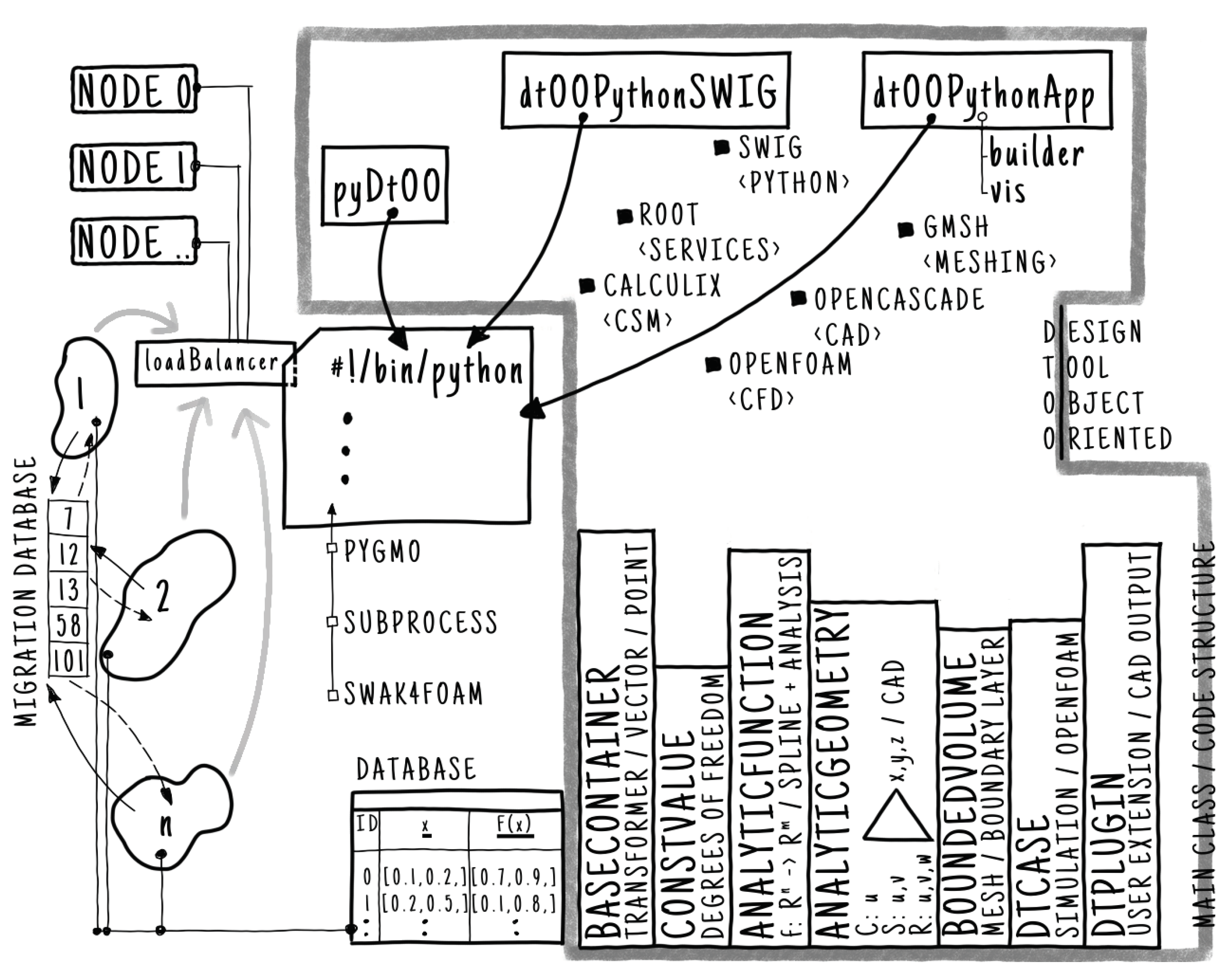
Figure 2.
Process of creating the runner blade: Sketchs I, II and III show the mean line, thickness distribution and combined blade, respectively, in a two-dimensional space.
Figure 2.
Process of creating the runner blade: Sketchs I, II and III show the mean line, thickness distribution and combined blade, respectively, in a two-dimensional space.
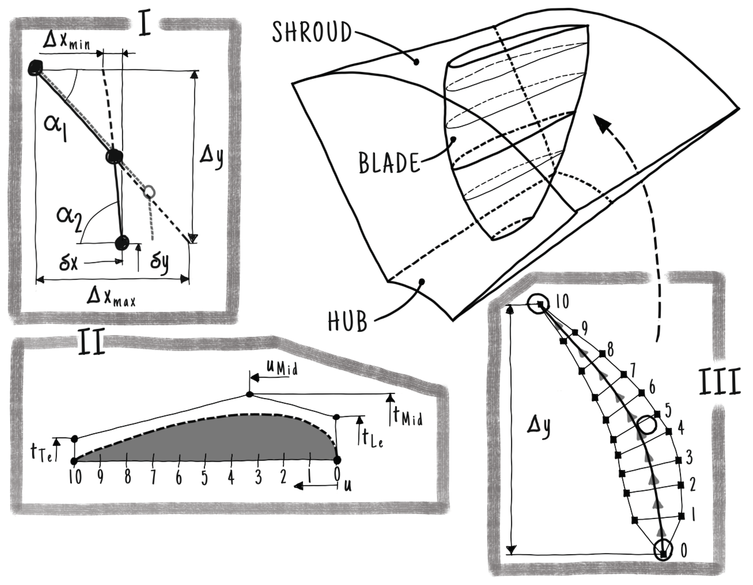
Figure 3.
Three-dimensional view of a candidate’s turbine blade with coordinates of extracted the flow field (left). Division of hexahedral boundary layer into FAs with their labels (right).
Figure 3.
Three-dimensional view of a candidate’s turbine blade with coordinates of extracted the flow field (left). Division of hexahedral boundary layer into FAs with their labels (right).
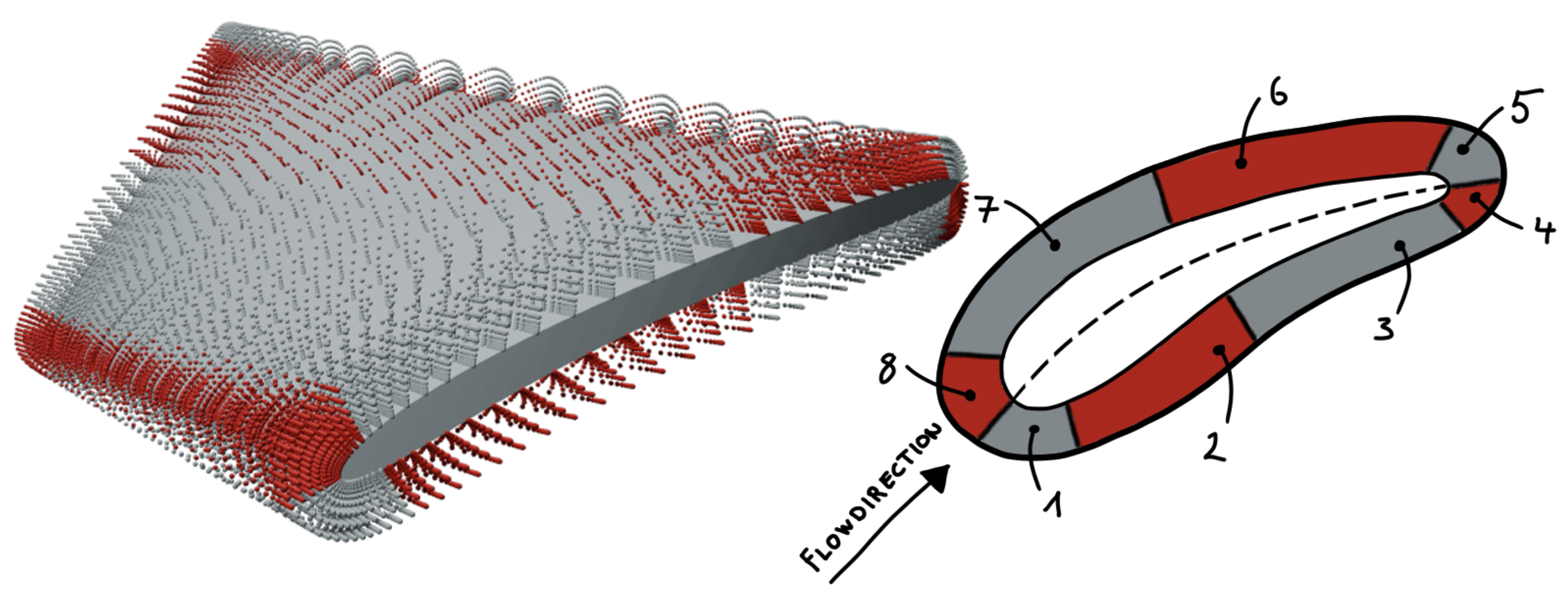
Figure 4.
Compression of data to latent-space representation (centered red box) by AE: Convolutional layers (four gray boxes on the left) compress the flow field data in lower dimensional space. Deconvolutional layers (four gray boxes on the right) reconstruct original data for training purposes.
Figure 4.
Compression of data to latent-space representation (centered red box) by AE: Convolutional layers (four gray boxes on the left) compress the flow field data in lower dimensional space. Deconvolutional layers (four gray boxes on the right) reconstruct original data for training purposes.
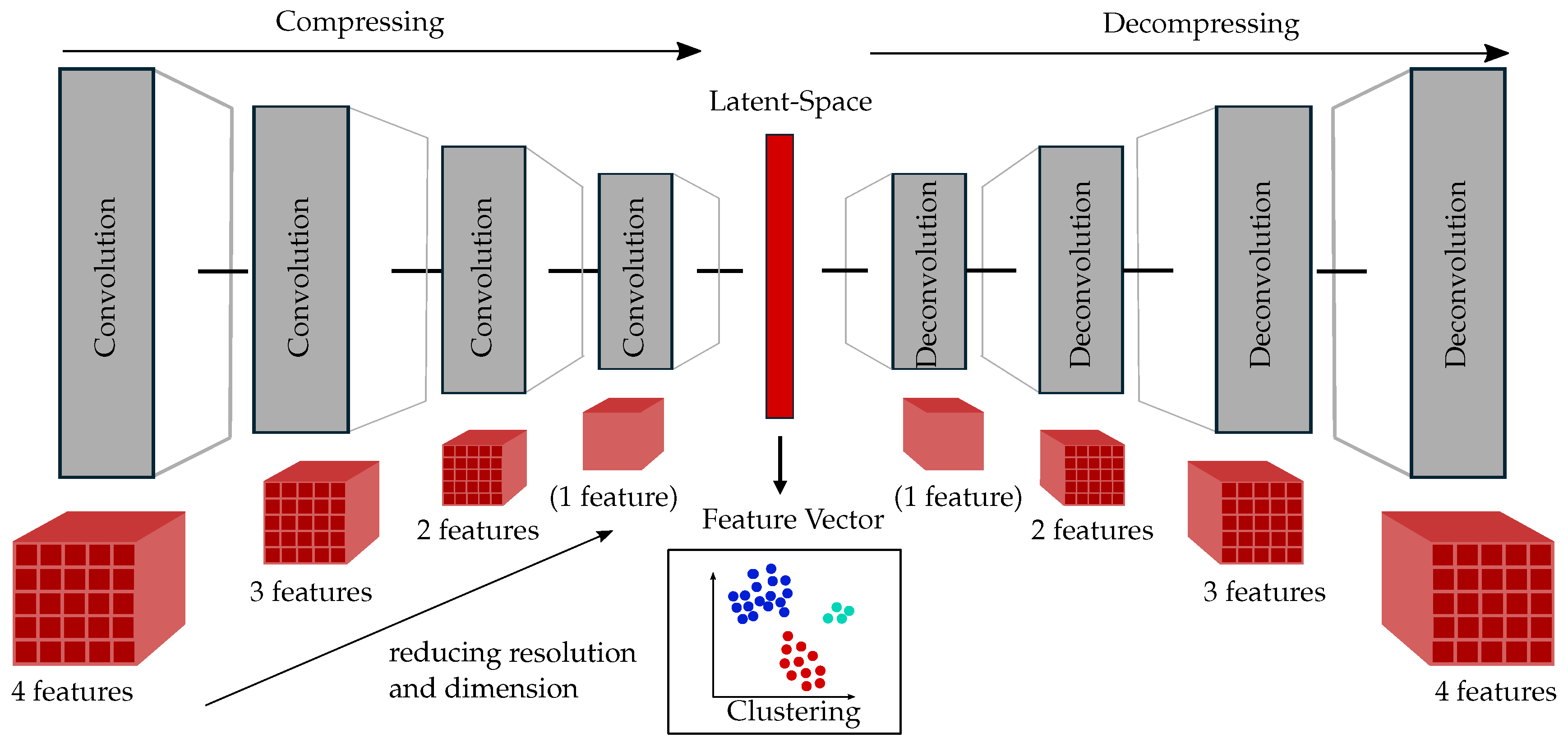
Figure 5.
Overview of the process to define the CI: The flow field of each FA (three-dimensional view on the left) is compressed to a latent space representation by an AE (visualized by gray and red boxes). Latent data is clustered to receive the CN in each FA. The three different clusters are visualized as blue, red and light green point clouds. All CNs together form the CI. (The schematic Figure shows the clustering for three FAs only).
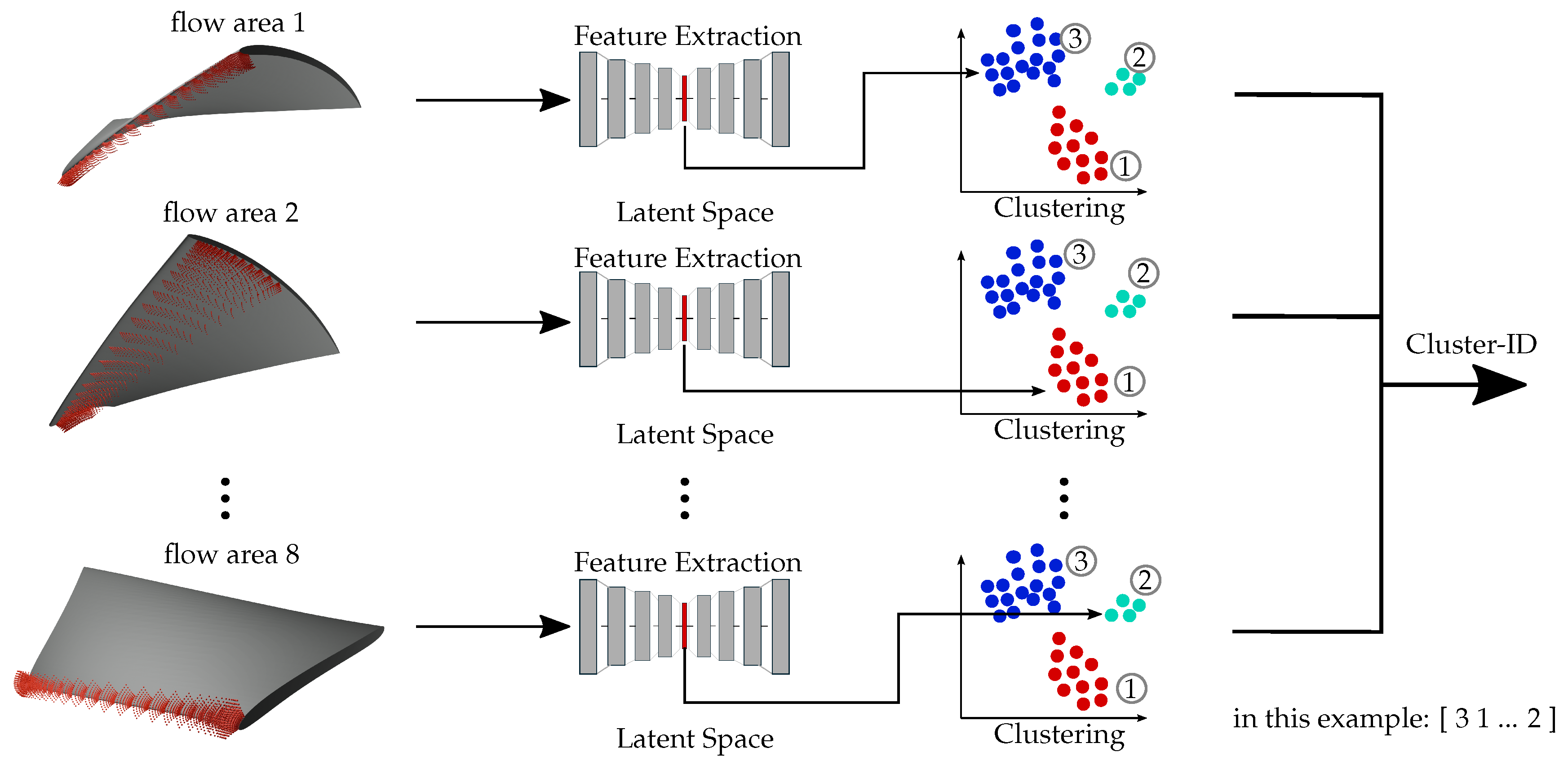
Figure 6.
Left (a): Fitness cavitation volume versus fitness efficiency for 500 individuals. Clusters of small gray dots are not visualized. Ten largest clusters are shown as big colored dots. Dots with same color means equal CI. Clustering algorithm uses k = 16. Right (b): Deviation between flow fields of same k. Deviation is estimated as the thickness of the envelope of all flow fields for each .
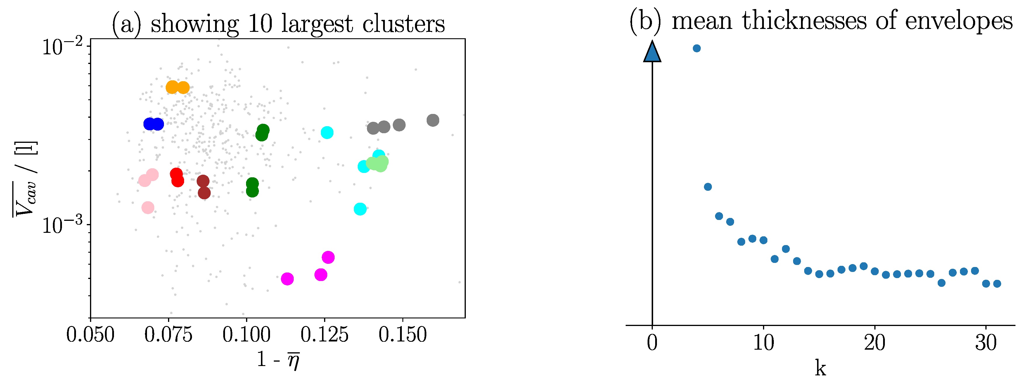
Figure 7.
Left (a): Superposed pressure values on the blade extracted from CFD for candidates that have equal CIs. Right (b): The thickness of the superposed pressure curves within one cluster.
Figure 7.
Left (a): Superposed pressure values on the blade extracted from CFD for candidates that have equal CIs. Right (b): The thickness of the superposed pressure curves within one cluster.
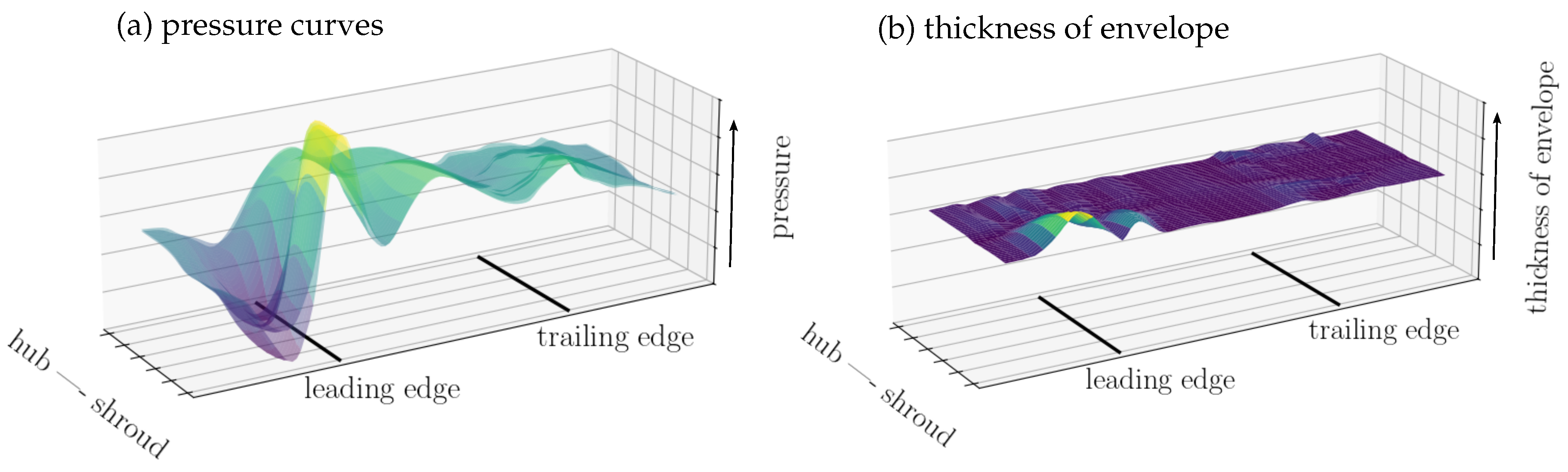
Figure 8.
CI prediction with NNs: Dataset generation by CFD simulation and flow field data clustering. For each FA, one NN predicts CN based on input parameter. All NNs together predict CI.
Figure 8.
CI prediction with NNs: Dataset generation by CFD simulation and flow field data clustering. For each FA, one NN predicts CN based on input parameter. All NNs together predict CI.
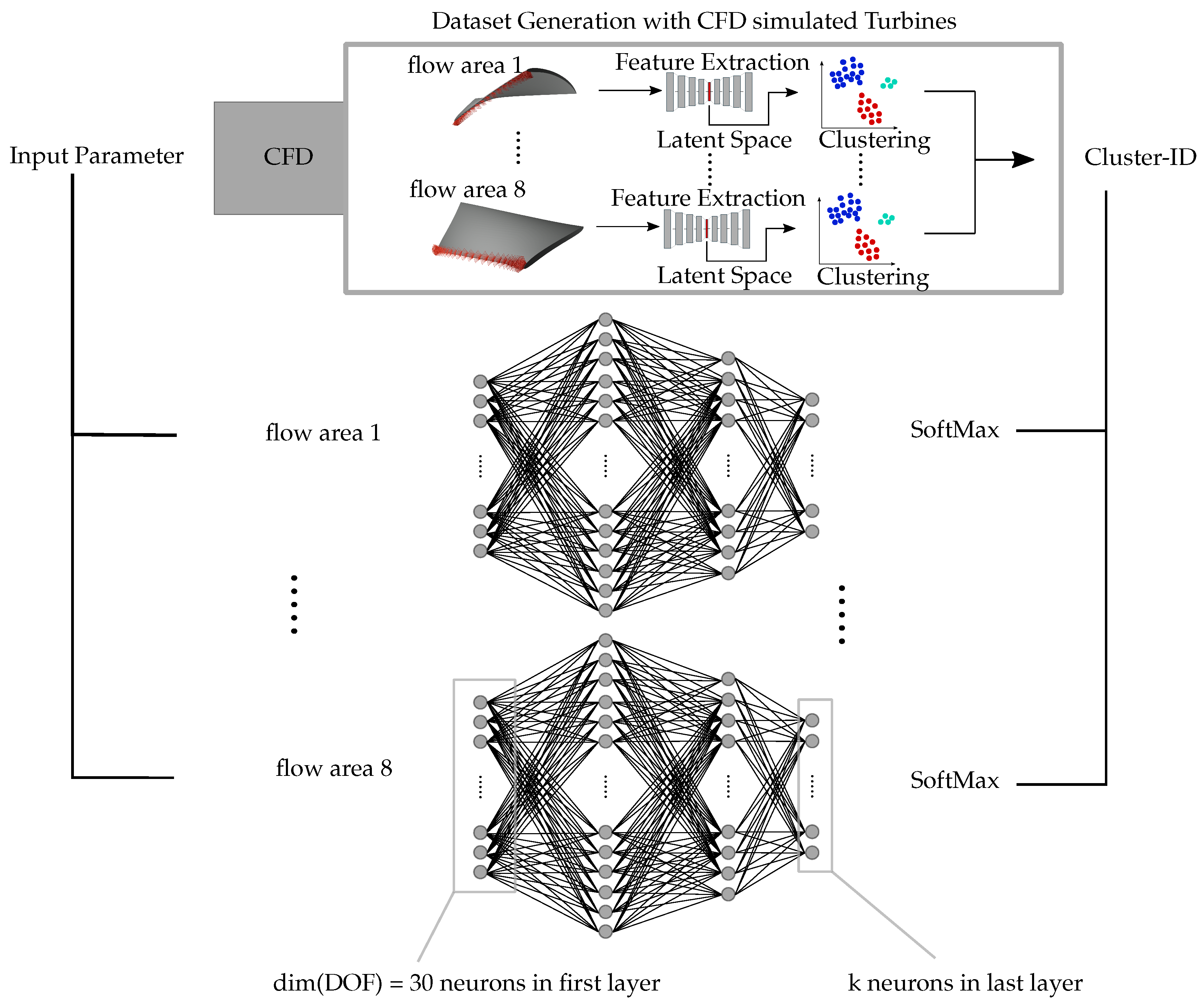
Figure 9.
Scheme Design Assistant: From NSGA-II suggested input parameters are evaluated by NNs. Based on predicted CI decision to simulate or to estimate is made. Fitness values are either extracted from Post-Processing CFD results or directly from design assistant’s estimation.
Figure 9.
Scheme Design Assistant: From NSGA-II suggested input parameters are evaluated by NNs. Based on predicted CI decision to simulate or to estimate is made. Fitness values are either extracted from Post-Processing CFD results or directly from design assistant’s estimation.
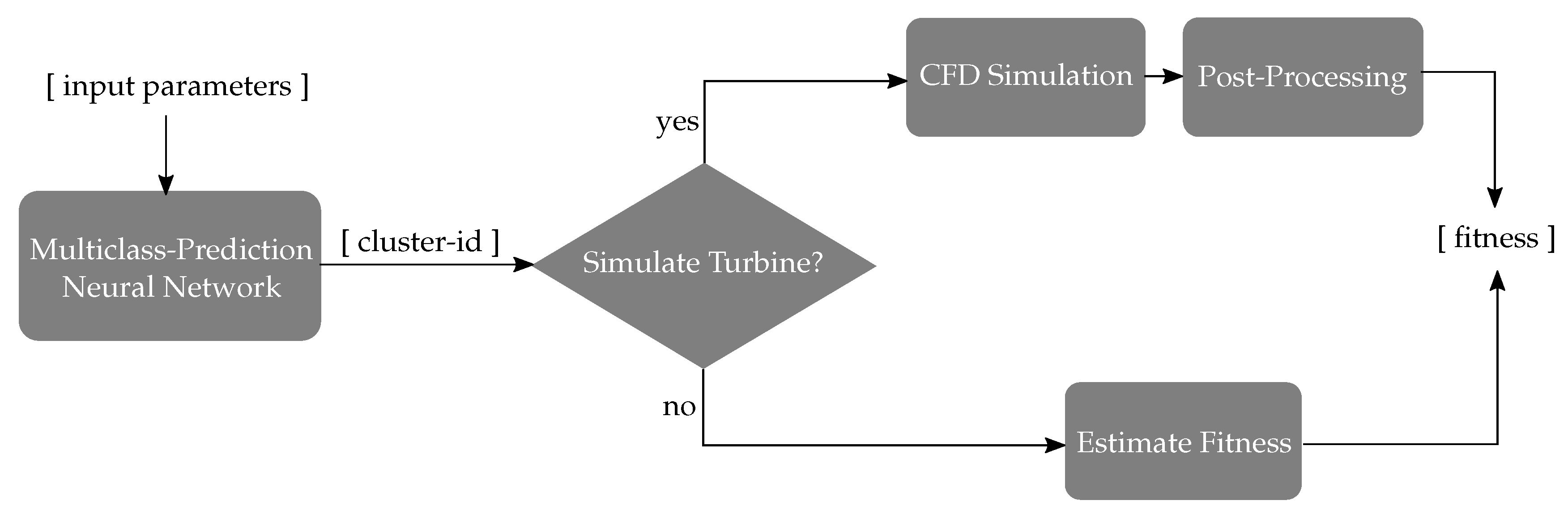
Figure 10.
Comparison between predicted and simulated fitness values sorted from worst to best prediction accuracy of the first 100 candidates. Clustering algorithm with k. Left (a): Design assistant without GPR. Right (b): Design assistant with GPR. Red and black horizontal lines mark the standard deviation and the mean of all simulated fitness values, respectively.
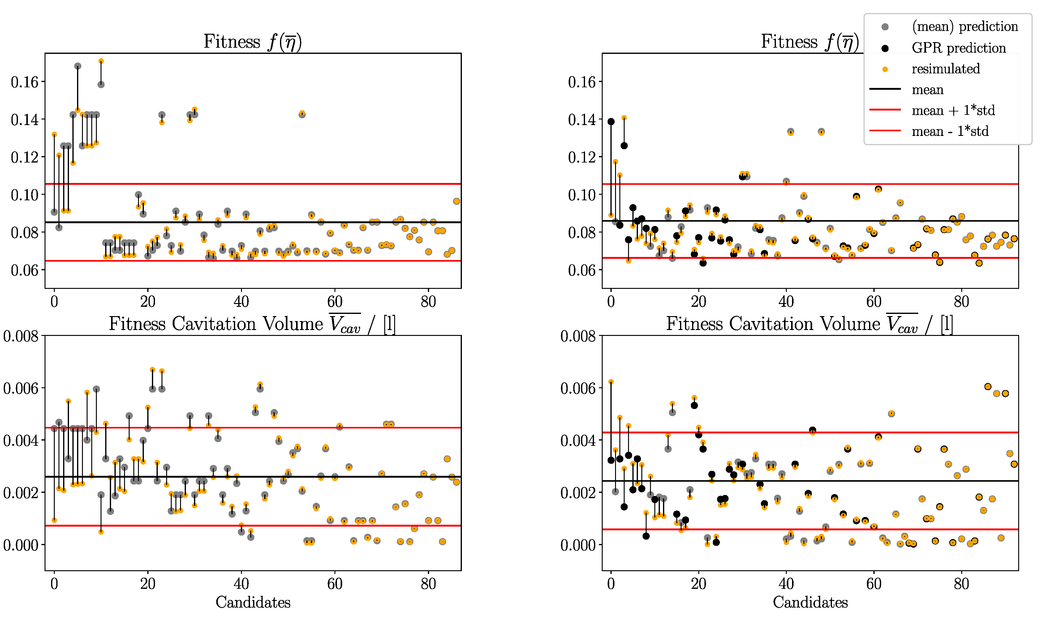
Figure 11.
Resimulated fitness values of previously predicted turbines in chronological order (orange). Green line marks the current threshold value. The dynamic threshold adaption is used here. Target of the design assistant is to avoid resimulated fitness values (orange) below the threshold line. The amount of resimulated turbines equals the amount of by the design assistant predicted turbines during optimization. These turbines do not require a CFD simulation during optimization and are only resimulated for evaluation purposes. In gray: All turbines’ fitness values.
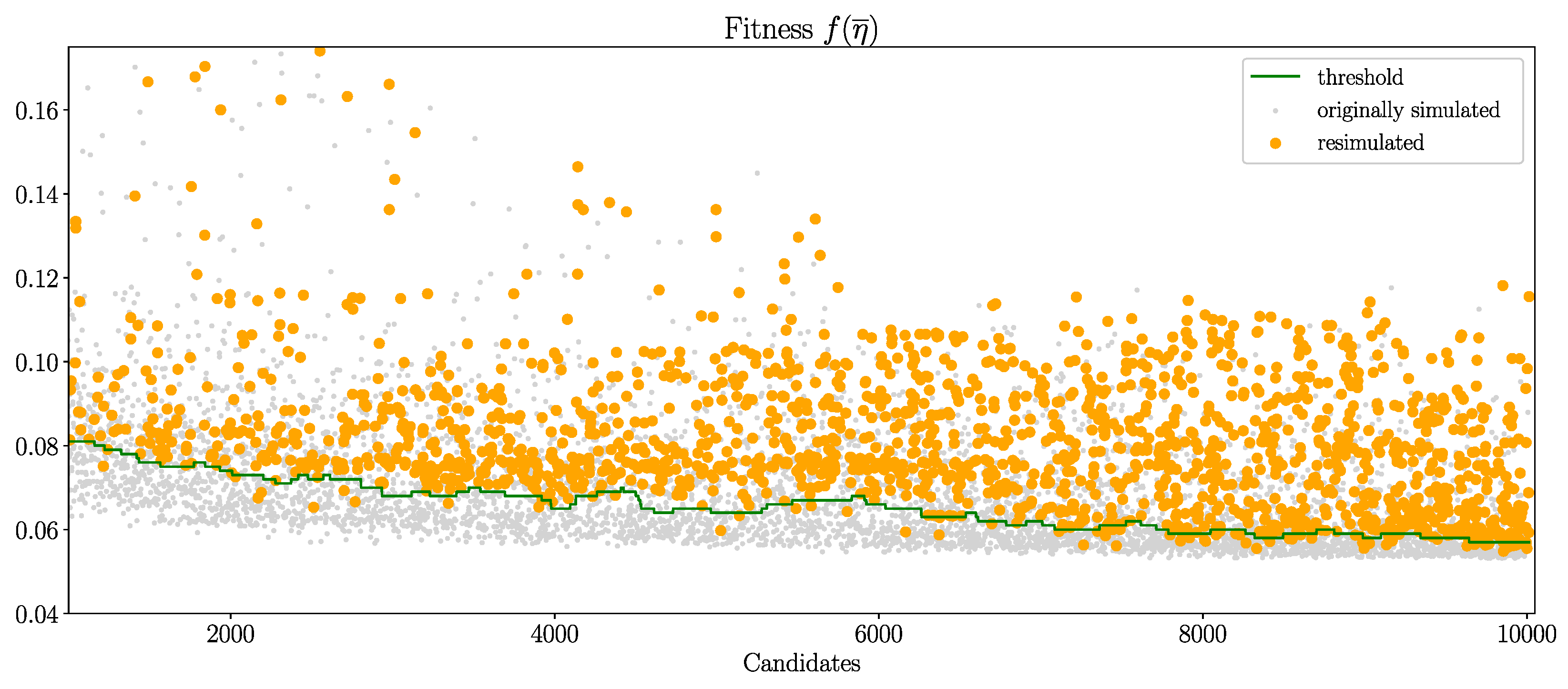
Figure 12.
Ratio of estimated turbines over the course of the simulation (a). Prediction deviation (b) during the optimization for and cavitation volume. Figure (c) shows the maximum amount of turbines sharing the same CI. For all three Figures the x-axis pictures the course of optimization by all suggested candidates.

Figure 13.
Pareto Front for Adapted Optimization: Circles mark the Pareto front of the initialization dataset of 1000 turbines. The triangles mark the new Pareto front after 10 000 individuals. Colors represent the head deviation. Target head is 2.4m.
Figure 13.
Pareto Front for Adapted Optimization: Circles mark the Pareto front of the initialization dataset of 1000 turbines. The triangles mark the new Pareto front after 10 000 individuals. Colors represent the head deviation. Target head is 2.4m.
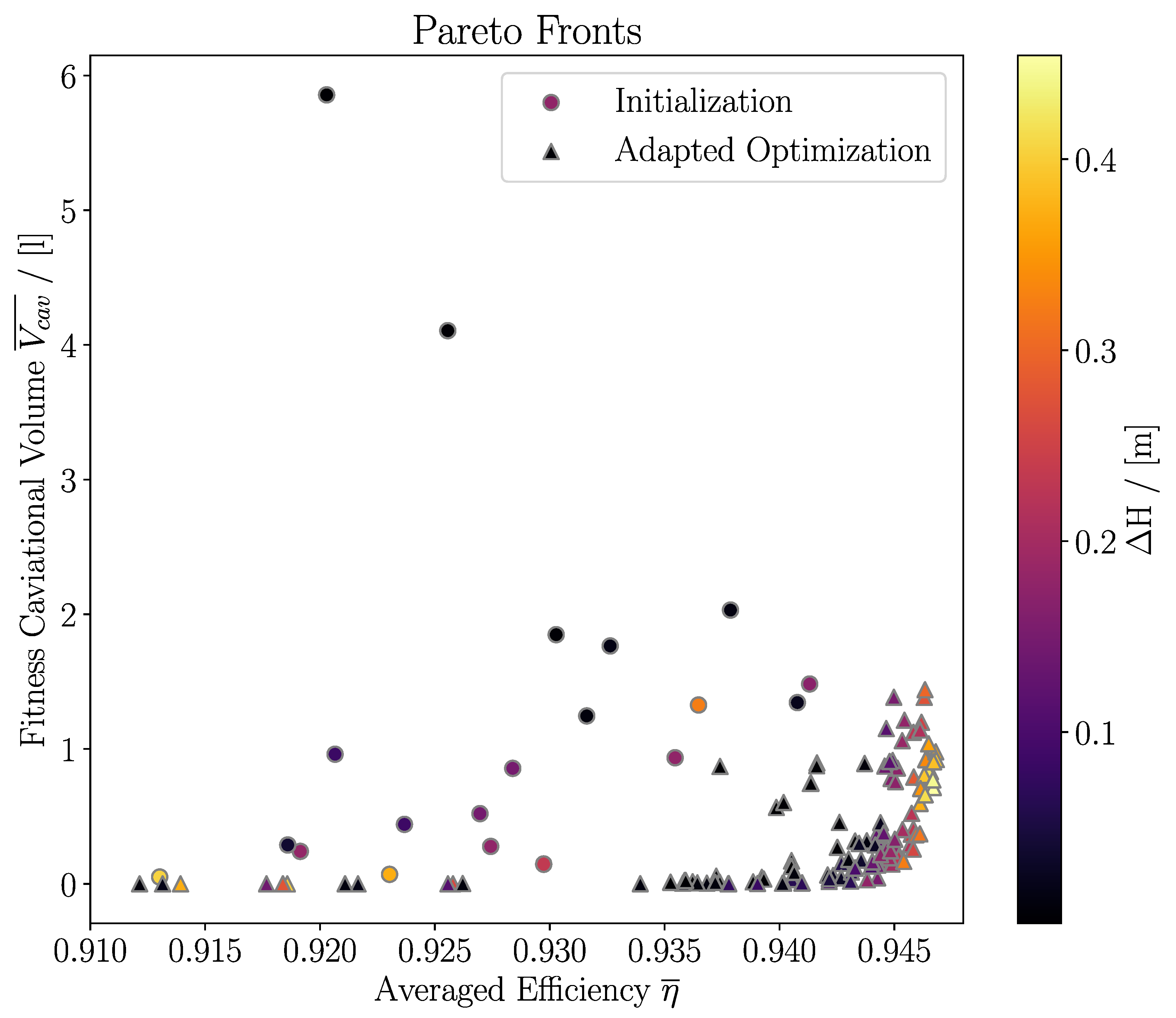

Table 1.
Fitness deviation of the first 100 predicted turbines for different values of k and with or without GPR for fitness values approximation
Table 1.
Fitness deviation of the first 100 predicted turbines for different values of k and with or without GPR for fitness values approximation
| Prediction Deviation | Deviation Fitness [%] | Deviation Fitness Cavitational Volume [l] |
|---|---|---|
| k = 16 | 0.32 | 0.38 |
| k = 16 | 0.28 | 0.44 |
| k = 20 | 0.495 | 0.54 |
| k = 20 | 0.29 | 0.25 |
Disclaimer/Publisher’s Note: The statements, opinions and data contained in all publications are solely those of the individual author(s) and contributor(s) and not of MDPI and/or the editor(s). MDPI and/or the editor(s) disclaim responsibility for any injury to people or property resulting from any ideas, methods, instructions or products referred to in the content. |
© 2024 by the authors. Licensee MDPI, Basel, Switzerland. This article is an open access article distributed under the terms and conditions of the Creative Commons Attribution (CC BY) license (http://creativecommons.org/licenses/by/4.0/).
Copyright: This open access article is published under a Creative Commons CC BY 4.0 license, which permit the free download, distribution, and reuse, provided that the author and preprint are cited in any reuse.


