
Submitted:
13 December 2024
Posted:
16 December 2024
You are already at the latest version
Abstract
Mounting pressure on emissions strictly connected to aviation has led to the development of SAF or Sustainable Aviation Fuel, an efficient tool by which aircraft operations are expected to cut emissions of climate altering agents considerably. According to several estimates, CO2 (carbon dioxide) emissions could be cut significantly, and the emission of sulfur compounds into the atmosphere could also be vastly reduced via SAF. Though this form of alternative fuel is still somehow challenged by costs, production availability and related concerns, it’s still expected to lead to considerable reductions in terms of aviation-related emissions over the course of forthcoming years. As of today, the attention is almost entirely focused on reduced emissions and how to make the implementation of SAF more efficient, but there’s a remarkable side effect of SAF’s replacement of conventional fossil fuels – namely, its characteristic carbon isotope fingerprint – which could be used to improve estimates and other models at least on local scales.
Keywords:
sustainable aviation fuel
; SAF
; aviation emissions
; CO2
; carbon isotopes
Introduction
Though safe and efficient, aviation is facing more and more pressure due to its relatively high passenger-to-emission ratio: though aviation-related emissions only constitute approximately 2.5% of global anthropogenic CO2 emissions, the percentage is not proportional to the total number of travelers by means of transport (Bergero et al., 2023, and references therein). The introduction of Sustainable Aviation Fuel (SAF) is now expected to turn the odds in aviation’s favor (Qasem et al., 2024), with an estimated reduction of up to 80% in CO2 emissions and some estimates providing even higher yields (Prussi et al., 2021). Carbon dioxide (CO2) is a powerful climate-altering agent due to its GWP (Global Warming Potential), which essentially indicates its capacity to perform a radiative forcing effect on Earth’s atmosphere, and therefore alter the climate of our planet (Liu et al., 2017). In addition to CO2, standard aviation fuel also results in the release of sulfur compounds which have a number of effects on the environment (Brown et al., 1996), effects SAF will attempt to tackle with reductions on that front as well. However, it’s worth noting that about two thirds of aviation’s radiative forcing effect is due to contrail cirrus clouds caused by dispersed water vapor, as largely highlighted in Lee et al. (2021). With respect to NOx (nitrogen oxides), which are also a byproduct of fossil fuels, it has been demonstrated that some alternate fuels could reduce their emissions (e.g., Timko et al., 2011), though this statement is not applicable to the broader family of alternate fuels as a whole (e.g., Khandelwal et al., 2019).
SAF is also set to change fuel lines of production, as small-scale production, even on a municipal scale, would be possible while fossil fuel production relies heavily on key spots located across the globe, such as the Middle East (Anser et al., 2020). One notable example of production on local scales would be the conversion of urban waste that would otherwise end up in landfills, accumulating over time and contributing to additional releases. SAF is also intended to reach impressive degrees of carbon neutrality (Braun et al., 2024). Broadly speaking, SAF constitute a family of fuels whose compositions, sources and production processes are heterogenous: in addition to the above-mentioned municipal waste, other sources such as pure food waste, oils/fats/greases and woody biomass have the potential to become SAF; this heterogeneity leads to numerous characteristics such as energy output, emission typology and intensity, and accordance with specific regulatory requirements (Undavalli et al., 2023, and references therein).
Speaking of CO2, there’s a side effect to the replacement of standard fuel with SAF, which also serves as an atmospheric tracer of said change. An atmospheric tracer is an element or compound, at times a physical parameter or even a combination of the two, which can pinpoint an emission source. In nature, CO2 isn’t always the same: the ratio between carbon-13 (13C) and carbon-12 (12C) isotopes in molecules changes depending on the emission source, while the carbon-14 isotope (14C) – due to its radioactive nature and consequent decay over the course of several thousands of years – is totally absent in fossil fuels, which are millions of years old.
The 13C/12C ratio of a given source, commonly reported as δ13C (delta carbon-13) in Geosciences, is calculated as a deviation per mille (‰) from the Vienna Pee Dee Belemnite standard (VPDB), which is the ratio extrapolated from the shell of a Late Cretaceous Belemnitella (d'Orbigny, 1840) cephalopod fossil from South Carolina (Craig, 1957). The δ13C of a given sample is calculated as follows:
For instance, fossil fuels have lower δ13CO2 compared to the standard ratios detectable in the atmosphere, and the overall CO2 concentration is also on the rise because of fossil fuels. In fact, the source apportionment made possible by δ13C analyses has been used to further demonstrate that the CO2 increase in the atmosphere is attributable to anthropogenic sources: as the absolute concentration of this compound increases, its isotopic fingerprint leans towards that of fossil fuels and diverges from standard Cenozoic Era values (Tipple et al., 2010).
The radioactive isotope 14C also has its own standard and observational parameters, named Δ14C, whose value in fossil fuels is −1000‰ due to the fact that said fuels are totally depleted in this isotope (Stuiver & Polach, 1977). The story behind 14C ratios in the atmosphere is intertwined with notable events of the past century: following the first use of atomic bombs in World War II and the consequent tests performed for decades by both the USA and USSR, as well as their allies, 14C values in the atmosphere have been perturbed and a milestone-study by Suess (1955) allowed to highlight the phenomenon. Following the reduction in atomic bomb tests, Δ14C have gradually reduced buy the so called “Suess Effect” is still considered when using radioactive carbon for purposes such as radiometric dating (Köhler, 2016). In the context of climate change research, this effect is used collectively to define both 13C and 14C composition perturbations caused by anthropic activities (Keeling, 1979).
Therefore, the carbon isotope fingerprint of SAF CO2 would possess certain properties, distinct from those of CO2 resulting from conventional fuel emissions: the analysis of carbon isotopes in the atmosphere could potentially pinpoint the influence of SAF’s introduction and improve local emission models in terms of source apportionment and sustainability. In a recent example by Kim et al. (2023), δ13CO2 and Δ14CO2 measurements have been efficiently integrated with CO (carbon monoxide, a typical byproduct of combustion processes) data to provide more details on source apportionment in the greater Los Angeles, CA area.
In a world that is working hard to struggle against the challenge of climate change, the study of carbon isotopes in the atmosphere provides very detail insights on environmental balance and human influence over them.
Methodology and Results
International networks of atmospheric observatories have been performing continuous measurements for decades; one notable example is NOAA’s (National Oceanic and Atmospheric Administration) Mauna Loa observatory, regarded in scientific research as the pillar of CO2 trend monitoring over the course of several decades (Keeling et al., 1976). The precision and accuracy of atmospheric measurements has to match strict standards due to the concentration of analyzed compounds: in order to detect changes of a few ppm or parts per million (10,000 ppm = 1%), instruments need to provide reliable results. For instance, detecting a 10 ppm increase in atmospheric CO2 from 415 to 425 ppm is the equivalent of detecting a compositional change from 0.0415% to 0.0425% in overall atmospheric data. In the past decade, technological breakthroughs have allowed the optimization and consequent testing of instruments capable of calculating δ13C in CO2, CH4 (methane) and other compounds (Rella et al., 2015; Dickinson et al., 2017). Thanks to these instruments, observatories can provide continuous and reliable data on carbon isotope fractionation, and by extent they can potentially detect the influence of SAF’s replacement over conventional aviation fuels. The accuracy and precision required to perform carbon isotope measurements is remarkable: in the case of CO2, if we were to assume an atmospheric composition of 425 ppm (0.0425%), carbon isotope detectors would then be capable of measuring deviations per mille from the VPDB standard of 0.01123720, which is the 13C:12C ratio used as reference. Since the industrial revolution, the average δ13CO2 in the atmosphere fell from −6.5‰ (note that it’s per mille, not per cent) to the currently observed value of ≈−8.5‰ (Graven et al., 2017, 2020).
In fossil fuels, δ13CO2 is known to fall in the −44‰ to −19‰ range, as demonstrated by Andres et al. (2000), while its Δ14CO2 counterpart is −1000‰. In the biosphere, the values are −29‰ to −12‰, and −150‰ to 150‰, respectively (Figure 1) (Bowling et al., 2008; Graven et al., 2020, and references therein). These values will be used as the baseline for a hypothetical example of data analysis on SAF vs. conventional fuels in the context of aviation.
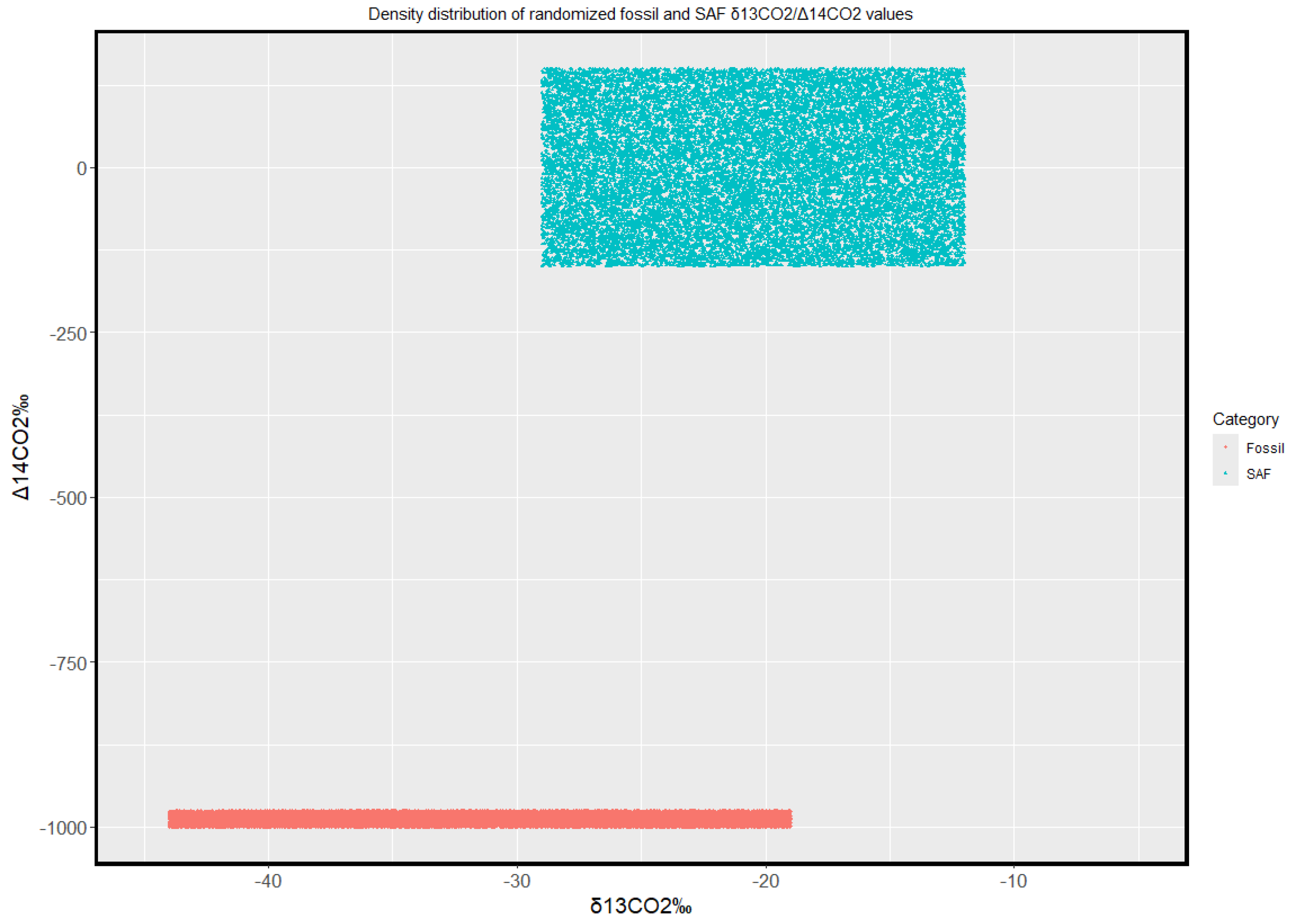
A simulation was performed in R v. 4.3.3 using 80,000 randomized values (40,000 per category, SAF and fossil, equally distributed between δ13CO2 and Δ14CO2) within the ranges stated above; Ggplot visual functions were integrated to improve the overall quality of the graph. A buffer zone of 25‰ (−1000‰ to −975‰) was assigned to Δ14CO2 values in order to make them noticeable, as a fixed value of −1000‰ would have lined them up on a defined δ13CO2 interval. The purpose of this graph (Figure 2) – which assumes that SAF, due to its variability, would reflect a wide range of δ13CO2 and Δ14CO2 values compatible in variability with Earth’s biosphere – is hereby presented as an example of SAF’s influence on atmospheric carbon isotope continuous measurements.
These are the end terms of fossil and SAF carbon isotope fingerprints: actual measurements, influenced by a number of factors as well as multiple sources, would result in intermediate values and the observed deltas would reflect the relative abundance of each source’s contribution to the total amount of CO2 being detected. The lower bound of Δ14CO2 however is to be considered an absolute boundary to the value of this parameter, as it’s effectively equal to zero.
With the two end members of the graph defined, it’s possible to assume that continuous carbon isotope measurements could detect the change in aviation fuels being used. The gradual replacement of standard fossil fuel with SAF would – in addition to lower emissions – result in a gradual shift from the lower end member of Figure 2 towards the higher. Though aviation’s contribution to global CO2 emissions is not particularly high in absolute terms, shifts could become more noticeable in the context of air quality/pollution measurements, where instruments would be placed close enough to airports to detect such changes. For the changes to be detectable, however, instruments would require to be in place prior to the substitution of fossil fuel with SAF, so that the change over time could be tracked efficiently.
Obviously, that needs more parameters being considered, such as dispersion models and outputs from other anthropic, as well as natural, sources. One extra factor in data variability over time could be seasonality: CO2, as well as other compounds, has seasonal cycles affecting absolute concentrations and isotopic ratios (Pataki et al., 2003).
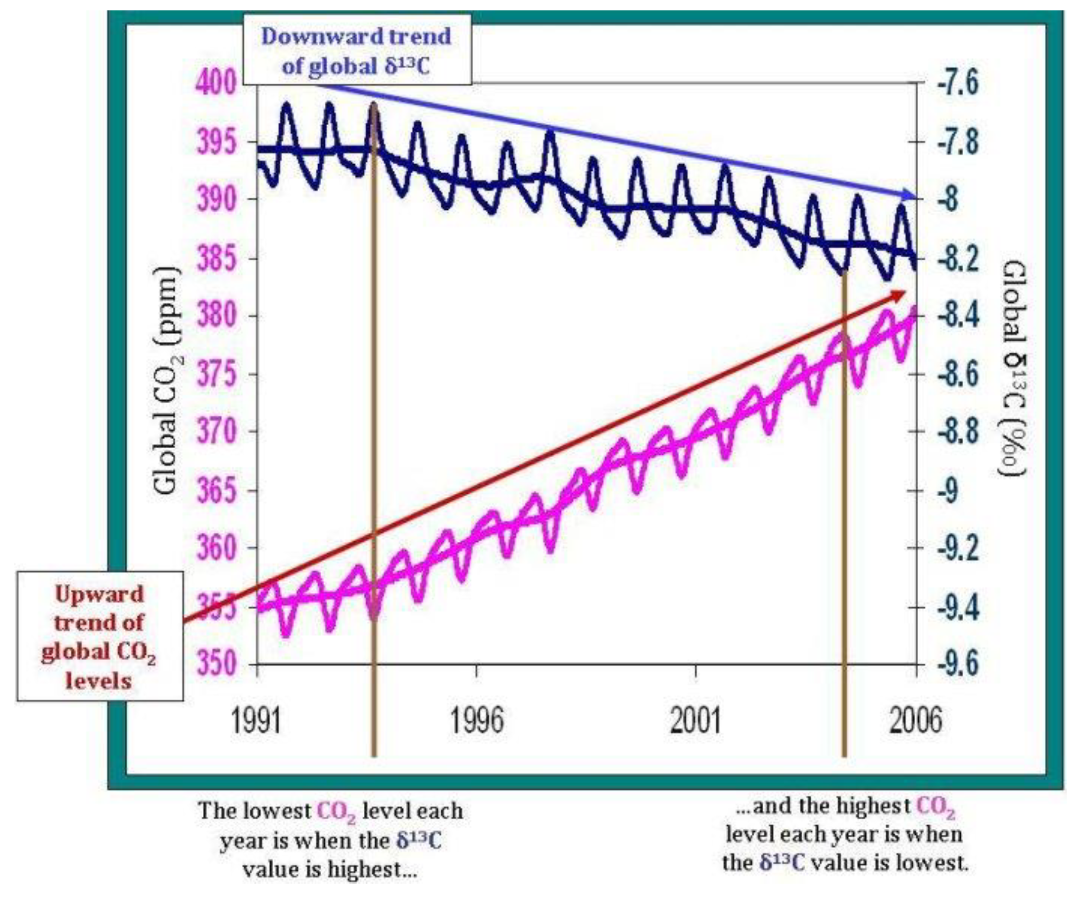
Figure 3.
The effects of photosynthesis and other processes driving seasonal trends in CO2 and δ13CO2 can be easily recognized. Note how low δ13CO2 values are tied to higher CO2 concentrations. From NOAA’s Global Monitoring Laboratory. https://gml.noaa.gov/ccgg/isotopes/c13tellsus.html.
Figure 3.
The effects of photosynthesis and other processes driving seasonal trends in CO2 and δ13CO2 can be easily recognized. Note how low δ13CO2 values are tied to higher CO2 concentrations. From NOAA’s Global Monitoring Laboratory. https://gml.noaa.gov/ccgg/isotopes/c13tellsus.html.
Another challenge that may have to be faced prior to the accomplishment of such accurate measurements on the fossil to SAF fuel transition are connected to Δ14CO2 estimations. In fact, though continuous measurements of this kind could be achieved via portable CRDS (Cavity Rind-Down Spectrometry) devices, the current state of the art of detailed 14C analyses relies on flasks being collected and sent to specific laboratories for processing (Yu et al., 2022, and references therein. On a regular basis, this implies that results are not instantaneous, and flasks have to be collected at selected time windows, meaning that any analysis has to take place when strictly necessary (in the case of SAF vs. fossil fuel evaluations, this could be performed for engine test beds, or even at selected airports during peaks of operating traffic).
The full implementation of continuous 14C measurements could therefore be a significant factor in discriminating SAF and fossil fuel, as 13C alone results in a partial overlap of isotopic values which can be easily recognized in Figure 2.
Though emissions in general contribute to global outputs and climate change, local effects are more susceptible to source apportionment. In the case of airports, the runways themselves are built to align with dominating wind directions in the area, and that in turn results into dispersions of pollutants and other byproducts of aviation fuel consumption that do not spread equally in all directions. The assessment of air quality around airports is generally performed on a per radius basis; in fact, the so called “near-airport” category range applies within a 6.21 miles radius from a given airport, regardless of the alignment of its runways. In the case of airports having two or more runways, dispersion models and consequent estimates on pollutant spreading would be more articulated. Several studies such as Carslaw et al. (2006) and Carslaw & Beevers (2013) have warned on the health hazards to workers and citizens alike spending extended periods of time in that radius, on the assumption that dispersion spreads pollutants in all directions. The implementation of continuous atmospheric measurements around airports, accounting for carbon isotope fractionation, could provide new insights on the actual influence of local air traffic and guide regulators towards improved policies.
Conclusions and Perspectives
Sustainable Aviation Fuels (SAF) are perhaps the key towards carbon neutrality, or near carbon neutrality, in the context of aviation. Their effective implementation is still challenged by costs, production chain logistics and availability, but all obstacles are in the process of being managed properly and it’s safe to foresee widespread use of SAF within years. Due to its nature, SAF possesses carbon isotope characteristics distinct from those of fossil fuels, in particular with respect to radiocarbon or carbon-14 (14C), which is effectively absent in fossil fuels. Carbon-13 (13C) isotope fractionation ratios partially overlap, but the combination of both parameters provides two distinct categories or “end members” in a plotted δ13CO2–Δ14CO2 graph which significantly improve the capacity to differentiate SAF from fossil fuel sources. Actual measurements aren’t likely to match any of the two end members, as detected carbon dioxide (CO2) will be result of different sources mixing in the atmospheric medium. The gradual shift from fossil fuels to SAF in aviation will result in lower emissions, but also in different CO2 isotopic fingerprints. These fingerprints may be of use in particular with respect to local air quality and pollution measurements around airports. The optimization of 14C measurements in particular could constitute a new technological breakthrough capable of bringing the source apportionment of CO2 to more efficient levels.
Declaration on AI Use
Though it’s not a requirement per se, the author would like to declare that at no point during the development of this paper AI and comparable tools were used. This statement applies to all aspects of this research, ranging from conceptualization to writing.
Acknowledgments
The author would like to thank the anonymous referee(s) for their insight and recommendations.
Conflicts of interest
The author declares no conflicts of interest regarding this article and its content. Moreso, the author declares that this paper is the result of an independent research endeavor and therefore does not represent the view of the two institutions the author is currently affiliated to.
References
- Andres, R.J.; Marland, G.; Boden, T.; Bischof, S. (2000). Carbon dioxide emissions from fossil fuel consumption and cement manufacture, 1751–1991, and an estimate of their isotopic composition and latitudinal distribution. In T. M. Wigley & D. S. Schimel (Eds.), The Carbon Cycle, pgs. 53–62. Cambridge: Cambridge University Press.
- Anser, M.K.; Abbas, Q.; Chaudhry, I.S. Khan, A. Optimal oil stockpiling, peak oil, and general equilibrium: case study of South Asia (oil importers) and Middle East (oil supplier). Environmental Science and Pollution Research, 2020; 27, 19304–19313. [Google Scholar] [CrossRef]
- Bergero, C.; Gosnell, G.; Gielen, D.; Kang, S.; Bazilian, M.; Davis, S.J. (2023). Pathways to net-zero emissions from aviation. Nature Sustainability 6, pgs. 404–414. [CrossRef]
- Braun, M.; Grimme, W.; Oesingmann, K. (2024). Pathway to net zero: Reviewing sustainable aviation fuels, environmental impacts and pricing. Journal of Air Transport Management 117, art.no. 102580. [CrossRef]
- Brown, R.C.; Anderson, M.R.; Miake-Lye, R.C.; Kolb, C.E.; Sorokin, A.A:; Buriko, Y.Y. (1996). Aircraft exhaust sulfur emissions. Geophysical Research Letters 23(24), pgs. 3603-3606. [CrossRef]
- Carslaw, D.C.; Beevers, S.D.; Ropkins, K.; Bell, M.C. (2006). Detecting and quantifying aircraft and other on-airport contributions to ambient nitrogen oxides in the vicinity of a large international airport. Atmospheric Environment 40, issue 28, pgs. 5424-5434. [CrossRef]
- Carslaw, D.C. & Beevers, S.D. (2013). Characterising and understanding emission sources using bivariate polar plots and k-means clustering. Environmental Modelling & Software 40, pgs. 325-329. [CrossRef]
- Craig, H. (1957). Isotopic standards for carbon and oxygen and correction factors for mass-spectrometric analysis of carbon dioxide. Geochimica et Cosmochimica Acta 12(1-2), pgs. 133-149. [CrossRef]
- Dickinson, D.; Bodé, S.; Boeckx, P. (2017). System for δ13C–CO2 and xCO2 analysis of discrete gas samples by cavity ring-down spectroscopy. Atmospheric Measurement Techniques 10(11), pgs. 4507–4519. [CrossRef]
- d’Orbigny, A.D. (1840). Paléontologie française; Terrains Crétacés, 1. Céphalopodes. Paris (Masson): pgs. 1-120.
- Graven, H.; Allison, C.E.; Etheridge, D.M.; Hammer, S.; Keeling, R.F.; Levin, I.; Meijer, H.A.J.; Rubino, M.; Tans, P.P.; Trudinger, C.M.; Vaughn, B.H.; White, J.W.C. (2017). Compiled records of carbon isotopes in atmospheric CO2 for historical simulations in CMIP6. Geoscientific Model Development 10(12), pgs. 4405–4417. [CrossRef]
- Graven, H.; Keeling, R.F.; Rogelj, J. (2020). Changes to Carbon Isotopes in Atmospheric CO2 Over the Industrial Era and Into the Future. Global Biogeochemical Cycles 34(11), e2019GB006170. [CrossRef]
- Keeling, C.D. (1979). The Suess effect: 13Carbon-14Carbon interrelations. Environment International 2(4–6), pgs. 229-300. [CrossRef]
- Keeling, C.D.; Bacastow, R.B.; Bainbridge, A.E.; Ekdahl, C.A.; Guenther, P.R.; Waterman, L.S; Chin, J.F.S. (1976). Atmospheric carbon dioxide variations at Mauna Loa Observatory, Hawaii. Tellus 28, pgs. 538-551. [CrossRef]
- Khandelwal, B.; Cronly, J.; Ahmed, I.S.; Wijesinghe, C.J.; Lewis, C. (2019). The effect of alternative fuels on gaseous and particulate matter (PM) emission performance in an auxiliary power unit (APU). The Aeronautical Journal 123(1263): pgs. 617-634. [CrossRef]
- Kim, J.; Miller, J.B.; Miller, C.E.; Lehman, S.J.; Michel, S.E.; Yadav, V.; Rollins, N.E.; Berelson, W.M. (2023). Quantification of fossil fuel CO2 from combined CO, δ13CO2 and ∆14CO2 observations. Atmospheric Chemistry and Physics 23, 14425–14436. [CrossRef]
- Köhler, P. (2016). Using the Suess effect on the stable carbon isotope to distinguish the future from the past in radiocarbon. Environmental Research Letters 11, no. 12. [CrossRef]
- Lee, D.S.; Fahey, D.W.; Skowron, A.; Allen, M.R.; Burkhardt, U.; Chen, Q.; Doherty, S.J.; Freeman, S.; Forster, P.M.; Fuglestvedt, J.; Gettelman, A.; DeLeón, R.R.; Lim, L.L.; Lund, M.T.; Millar, R.J.; Owen, B.; Penner, J.E.; Pitari, G.; Prather, M.J.; Sausen, R.; Wilcox, L.J. (2021). The contribution of global aviation to anthropogenic climate forcing for 2000 to 2018. Atmospheric Environment 244, art.no. 117834. [CrossRef]
- Liu, W.; Zhang, Z.; Xie, X.; Yu, Z.; von Gadow, K.; Xu, J.; Zhao, S.; Yang, Y. (2017). Analysis of the Global Warming Potential of Biogenic CO2 Emission in Life Cycle Assessments. Scientific Reports 7, art.no. 39857. [CrossRef]
- Pataki, D.E.; Bowling, D.R.; Ehleringer, J.R. (2003). Seasonal cycle of carbon dioxide and its isotopic composition in an urban atmosphere: Anthropogenic and biogenic effects. Journal of Geophysical Research: Atmospheres 108, D23. [CrossRef]
- Prussi, M.; Lee, U.; Wang, M.; Malina, R.; Valin, H.; Taheripour, F.; Velarde, C.; Staples, M.D.; Lonza, L.; Hileman, J.I. (2021). CORSIA: The first internationally adopted approach to calculate life-cycle GHG emissions for aviation fuels. Renewable and Sustainable Energy Reviews 150, art.no. 111398. [CrossRef]
- Qasem, N.A.A.; Mourad, A.; Abderrahmane, A.; Said, Z.; Younis, O.; Guedri, K.; Kolsi, L. (2024). A recent review of aviation fuels and sustainable aviation fuels. Journal of Thermal Analysis and Calorimetry. [CrossRef]
- Rella, C.W.; Hoffnagle, J.; He, Y.; Tajima, S. (2015). Local- and regional-scale measurements of CH4, δ13CH4, and C2H6 in the Uintah Basin using a mobile stable isotope analyzer. Atmospheric Measurement Techniques 8(10), pgs. 4539–4559. [CrossRef]
- Stuiver, M. & Polach, H.A. (1977). Discussion: Reporting of 14C Data. Radiocarbon 19(3), pgs. 355–363. [CrossRef]
- Suess, H.E. (1955). Radiocarbon Concentration in Modern Wood. Science 122, issue 3166, pgs. 415-417. [CrossRef]
- Timko, M.T.; Herndon, S.C.; de la Rosa Blanco, E.; Wood, E.C.; Yu, Z.; Miake-Lye, R.C.; Knighton, W.B.; Shafer, L.; DeWitt, M.J.; Corporan, E. (2011). Combustion Products of Petroleum Jet Fuel, a Fischer–Tropsch Synthetic Fuel, and a Biomass Fatty Acid Methyl Ester Fuel for a Gas Turbine Engine. Combustion Science and Technology 183(10), pgs. 1039–1068. [CrossRef]
- Tipple, B.J.; Meyers, S.R.; Pagani, M. (2010). Carbon isotope ratio of Cenozoic CO2: A comparative evaluation of available geochemical proxies. Paleoceanography and Paleoclimatology 25(3). [CrossRef]
- Undavalli, V.; Gbadamosi Olatunde, O.B.; Boylu, R.; Wei, C.; Haeker, J.; Hamilton, J.; Khandelwal, B. (2023). Recent advancements in sustainable aviation fuels. Progress in Aerospace Sciences 136, art.no. 100876. [CrossRef]
- Yu, M.-Y.; Lin, Y.-C.; Zhang, Y.-L. (2022). Estimation of Atmospheric Fossil Fuel CO2 Traced by Δ14C: Current Status and Outlook. Atmosphere 13(12), 2131. [CrossRef]
Figure 1.
Carbon-13 (up) and carbon-14 (down) fractionations in different environments. For the purpose of this research, it is assumed that SAF would fall in the broader Biosphere category ranges. From Graven et al. (2020), modified.
Figure 1.
Carbon-13 (up) and carbon-14 (down) fractionations in different environments. For the purpose of this research, it is assumed that SAF would fall in the broader Biosphere category ranges. From Graven et al. (2020), modified.
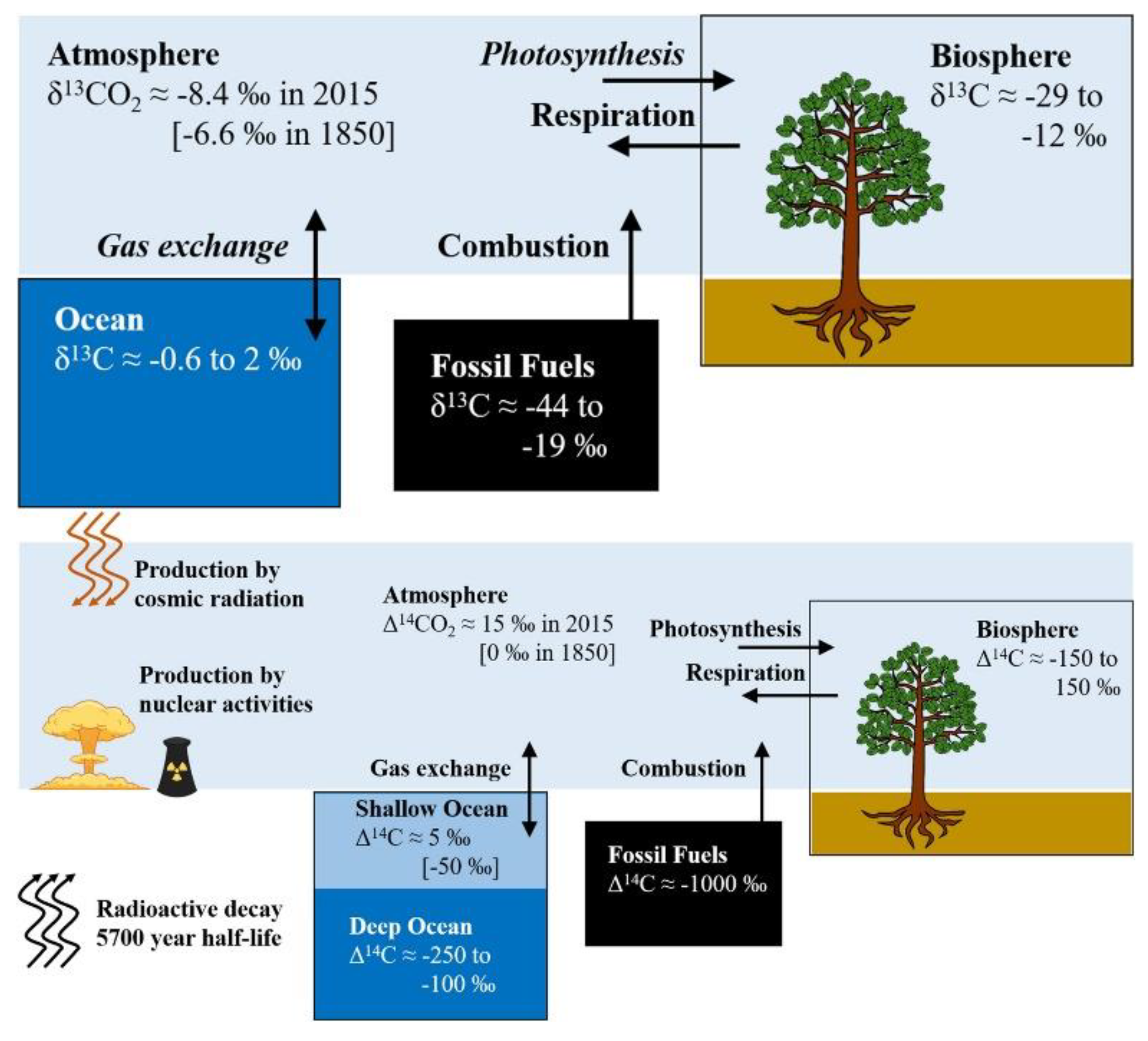
Figure 2.
Plotted example of δ13CO2 and Δ14CO2 values, divided by category of fuel (SAF vs. fossil). Please note that a 25‰ buffer zone was added to fossil fuel Δ14CO2. Though this was done for data visualization purposes, it does show a plausible scenario of contamination between aviation fuel CO2, and CO2 attributable to other sources.
Disclaimer/Publisher’s Note: The statements, opinions and data contained in all publications are solely those of the individual author(s) and contributor(s) and not of MDPI and/or the editor(s). MDPI and/or the editor(s) disclaim responsibility for any injury to people or property resulting from any ideas, methods, instructions or products referred to in the content. |
© 2024 by the authors. Licensee MDPI, Basel, Switzerland. This article is an open access article distributed under the terms and conditions of the Creative Commons Attribution (CC BY) license (http://creativecommons.org/licenses/by/4.0/).
Copyright: This open access article is published under a Creative Commons CC BY 4.0 license, which permit the free download, distribution, and reuse, provided that the author and preprint are cited in any reuse.


