Submitted:
14 December 2024
Posted:
16 December 2024
You are already at the latest version
Abstract
The present paper introduces the so-called scintillators footprints, made of schemes showing XRF-escape peaks and their relative emission intensities in the energy range of interest for nuclear medicine SPECT and PET. A footprint describes the suitability of a scintillator for quantitative investigation with the best possible detectabilility. Sixteen scintillation materials have been identified in Literature, characterized by effective atomic number ranging between 22 to 75. The footprints of NaI:Tl and BGO, confirm the best suitability for quantitative spectral analisys at 140.5 keV and 511 keV, respectively. Moreover, for the low-Z eff scintillators like CaF 2 and CMSM, the XRF-escape effect is foresee irrelevant even at 140.5 keV, due to the small energy value of X-ray fluorescences.
Keywords:
gamma-ray scintillation detector
; XRF-escape
; SPECT
; PET
1. Introduction
The purpose of this paper is to foresee, for sixteen scintillators, information about the distribution of XRF-escape peaks within the given energy Region of Interest (RoI). The last are the ones typical interest in nuclear medicine imaging, and are located around the photoelectric peaks at 140.5 or 511 keV, from 99-Tc decay and β+ annihilation radiation, respectively. The RoI at 661.6 keV, was added to present study because it is usually used as standard reference in gamma-ray spectrometry.
This study summarizes the values of energy and relative intensities of XRF-escape peaks for 16 scintillation materials, included the most widely used ones, and describes, at a glance, the distribution of these escape-peaks along with the schematized scintillator response-functions for gamma-ray energy up to about 700 keV.
From a spectrometric point of view, the crowding of XRF-escape peaks from scintillator components in the valley between Compton-edge and full-energy peak make difficult the peak search and identification and the assessment of their area, that is crucial for quantitative spectrometry.
Figure 1 displays the distributions of K-, L- and M-shell edges energy values for all the elements whose atomic number Z ranges between 4 and 83. Data have been arranged from Ref [1].
1.1. The Search for New Scintillators
After Robert Hofstadter who introduced NaI:Tl in 1948 [2], the studies on new scintillators have never discarded worldwide. A plurality of parameters are usually evaluated when designing new scintillators for nuclear medicine imaging, or gamma ray spectrometry in other fields. Among these parameters, the following should be mentioned, but not in order of importance: the light output per unit of deposited energy, the scintillation decay-time constant, the wavelength range of the scintillation light and the corresponding transmittance trend, the energy resolution for gamma emissions of the radioisotope of preferential use, the detection efficiency, as well as basic mechanical, optical and physical characteristics relating to the crystal growth processes and their post-production processing. As one can see, the optimization of all these parameters is very complicated due to the many restrictions to take into account at the same time.
2. Materials and Methods
In Figure 1 it is to be noted that, starting from the uppermost K orbitals, between the shells, a decrease of at least one order of magnitude in the characteristic energy values is observed for the same value of Z [1]. Therefore, the considerations regarding the shift of the centroids of the XRF-escape peaks can be reasonably limited to the emissions of the K orbitals alone since the effects of such dislocations are quite predominant compared to the rest of the orbitals.
It should also be noted that the intensity of X-rays generated by the K orbitals are prevalent, even due to fluorescence-yield value ωK(Z) , that is much higher compared to the yields of other orbitals ωL(Z) and ωM(Z) [1].
2.1. XRF-Escape Peak-Energy Calculation
For an hypothetic single-element scintillator, one can write the energies of the photons involved in a K-Xray escape process as in the Eq.(1):
where the symbols represent the values of photon energy as follows:
EEsc = Eγ – EXrf ,
EEsc : escaping X-ray,
Eγ : incoming photon,
EXrf : X-ray fluorescence from the given K atomic shell.
Since, in a first approximation, EXrf is a quantity characteristic of the element constituting the scintillator, therefore a peak will appear in the gamma pulse-height spectrum, to the left of Eγ , whose centroid is coincident exactly with EEsc . But, since in a second approximation, EXrf is characterized by a certain spread, also depending on Z , corresponding to the energy levels of the different orbitals of K-shell for the element in question, a certain additional spread must be expected in the values of EEsc (also increasingly dependent on Z ) which, in principle, will worsen the energy resolution value expected for single-photons falling in full-energy peaks.
Since a fluorescence photon is emitted following ionization, one must have:
Eγ ≥ EXrf .
In other words, the XRF-emission is a threshold-process conditioned by the occurrence of Eq.(2).
In the case of a scintillator with Nc ≥ 2 components, and adding a term of percent abundance for the ith element in the mixture constituting the scintillator, we can derive the Eq.(3) from Eq.(1).
The Eq.(3) describes, if the value of the energy of the incident photon Eγ has been set, the pairs of values EEsc(i) and Ab(i) which characterize the XRF-escape emission and the composition of a certain scintillator for each component:
EEsc (i) = Eγ – EXrf (i) , Ab(i) ( i = 1, … , Nc )
Such couples of values, represent in the (photon energy, abundance) Cartesian plane the so-called scintillator footprint, describing the positions expected for the XRF-escape peaks of components.
In the Figs. such positions are compared with those of full-energy peaks, Eγ , and of Compton edges, Eγ’ , calculated, the latter, using the well known Eq.(4) with θ = π (see Ref.[3], p.51):
where: θ is the angle between the directions of the photons γ and γ’ , and m0 c2 stays for the electron rest-mass (511 keV).
Eγ’ = Eγ / [ 1 + ( Eγ ( 1 - cos θ ) / m0 c2 ) ] ,
2.2. Evolution of the Arsenal Available for Medical Application
Following the introduction of NaI:Tl detectors [2], the first advance in the field of medical imaging with radionuclides was achieved starting from the late 1940s, particularly by B. Cassen at LBNL, California, USA, whose research was oriented towards intraoperative devices for tracking radioactive substances within biological organisms, based on ZnS and CaWO4 scintillators [4].
At this time R. Hofstadter, at Princeton, New Jersey, USA, was working on NaI:Tl scintillators, whose commercial availability within PMT-based detectors allowed B. Cassen the construction of a human-scale whole-body scanner [5].
Efforts dedicated to nuclear medicine development also benefited from the fundamental contemporary discoveries of technetium radioisotopes by C. Perrier and E. Segrè as well as of those of iodine by G. Seaborg and J. Livingood. Some radioisotopes of these elements now cover almost all diagnostic needs in nuclear medicine.
After M. Casey and R. Nutt, two important innovations have been introduced, particularly for PET systems, regarding the use of block-detectors, based on BGO scintillators, and, mostly, the scintillation crystals made of array of scintillators [6]. The high Z value of bismuth become more adequate to the photon energy to be detected with respect to foregoing NaI:Tl experimental assemblies, and the fine scintillators segmentation witch increases the ratio of XRF-escapes events to total ones.
2.3. Selection of Scintillators for Present Study
An extensive bibliographic investigation, concerning the elemental composition of many scintillators, was conducted, aimed to carrying out the present study. The Literature inquiry has found 149 materials including the most popular ones, according to the following specifications: (i) inorganic mixtures, (ii) known compositions by weight or stoichiometry, (iii) suitability for gamma-ray spectrometry, (iv) values of Z ≤ 83.
Among the materials exiting the selection, sixteen have been enrolled in present study, whose main data are reported in Table I, where the number of components is between 2 and 7, and Zeff values, calculated according to Ishii and Kobayashi (see Ref.[10], p.251), are distributed, with a certain equidistance, between 22 and 76.

Table I.
List of the 16 inorganic scintillators selected for present study. Mixtures are characterized by number of elements from 2 to 7, and by Zeff values ranging from 22 to 76.
Table I.
List of the 16 inorganic scintillators selected for present study. Mixtures are characterized by number of elements from 2 to 7, and by Zeff values ranging from 22 to 76.
| Mixture/Compound | Formula | Z of Components (1) | Composition (% wt) (1) | Zeff (2) | Ref. |
| CaF2 | CaF2:Eu1% | 20; 9; 63. | 50.8195; 48.1805; 1. . | 22.18 | [11] |
| GaO | Ga2O3:Sn2% | 31; 8; 50. | 72.9055; 25.0945; 2. . | 29.90 | [12] |
| CMSM | Ca2MgSi2O7:Ce_Eu1% | 20; 12; 14; 8; 58, 63. | 28.8133; 8.73698; 20.1912; 40.2586; 1.; 1. . | 23.93 | [13] |
| RCB | RbCaBr3:Eu1% | 37; 20; 35; 63. | 23.1653; 10.8628; 64.9719; 1 . | 35.48 | [14] |
| YSO | Y2SiO5:Ce0.2% | 39; 14; 8; 58. | 62.0706; 9.8039; 27.9254; 0.2 . | 34.78 | [15] |
| NaI | NaI:Tl1% | 11; 53; 81. | 15.1840; 83.8160; 1 . | 50.91 | [16] |
| CsI | CsI:Tl1% | 55; 53; 81. | 50.6433; 48.3567; 1 . | 54.59 | [17] |
| LaCl | LaCl3:Ce10% | 57; 17; 58. | 50.9724; 39.0276: 10 . | 50.58 | [18] |
| GYAGG | (Gd0.5Y0.5)3 Al2 Ga3O12:Ce1%Mg0.1% | 64; 39; 13; 31; 8; 58; 12. | 28.2984; 15.9993; 6.47406; 25.0944; 23.0338, 0.1 , 0.1 . | 48.35 | [19] |
| CeF3 | CeF3 | 58; 9. | 71.0847; 28.9253 . | 53.26 | [20] |
| LuYGAGG | (LuYGd)3(GaAl)5O12:Ce1% | 71; 39; 64; 31; 13; 8; 58. | 26.8016; 13.6187; 24.0877; 17.8004; 6.8884; 9.8032; 1. . | 58.17 | [21] |
| LYSO | Lu2Y2SiO5:Ce1% | 71; 39; 14; 8; 58. | 54.4856; 27.6858; 4.3729; 12.4557; 1.0 . | 61.82 | [8] |
| LuYAP | (Lu0.7Y0.3)AlO3: Ce0.4% | 71; 39; 13; 8; 58. | 54.4273; 11.8526; 11.9903; 21.3298; 0.4 . | 61.34 | [9] |
| LSO | Lu2SiO5:Ce1% | 71; 14; 8; 58. | 75.6381; 6.0706; 17.2913; 1 . | 66.31 | [7] |
| LHO | Lu2Hf2O7 | 71; 72, 8. | 42.7317; 43.5921; 13.6762 . | 68.93 | [22] |
| BGO | Bi4Ge3O12 | 83; 32; 8. | 67.0989; 17.4890; 15.4112 . | 75.23 | [23] |
(1) For each scintillator the elements are reported in the same order of the respective formula, from left to right. If the reference gave only the chemical formulas of the mixtures, then the elemental compositions in percent by weight (%wt) were calculated at Chemical Portal - WebQC.Org. Available at: https://www.webqc.org/ (Accessed: September 2024). (2) Calculated according to Ishii and Kobayashi (see Ref.[10], p.251).
2.4. Scintillators Footprints
From the above it emerges that, without performing accurate Monte Carlo calculations, it is impossible to estimate the fraction of incident photons that give rise to the XRF-escape process. Infact, the factors affecting that fraction are multiple and can be grouped as follows:
- elemental composition, geometrical shape and dimensions of the scintillator;
- radioisotopic composition, geometrical shape and dimensions of the particle source(s);
- particles spectrum(a) from source(s);
- complete spatial map including source(s), detector, shielding, walls, etc … .
However, for simple cases of monoenergetic gamma-ray point source with a hypothesis of scintillator composition, it is possible to predict the ability of an assembly to best carry out quantitative analises.
Present study allows predicting that capability at 140.5 keV (from Tc-99 β-- decay) and at 511 keV (from ε F-18 decay). Furthermore the assessment is performed at 661.6 keV (from β-- Cs-137 decay).
By using the composition data associated with the selected compounds, plots have been produced containing XRF-escape footprints, characteristics of the components at the given energies, superimposed on the stylized pulse-height spectra. The last represent the Compton-continuum with its edge and the full-energy-peak (dashed curves) that constitute the ideal limits of a valley.
The energy-values of XRF-escape peaks from the mixture components are represented by bold segments ended by solid triangles. Such extremities represent the characteristic energies of Kα2 line (to the left) and of Kedge (to the right) for the given element. The XRF-escape photons from the rest of K-shell orbitals by increasing energy (i.e.: Kα1, Kβ3, Kβ1 and Kβ2 , respectively) will evidently fall at intermediate points of that segment (see Eq.(1)), whose intensities are reported in [1]. It is to be noted that for elements having values of Z small, the triangular symbols can appear coincident because of the size of symbols itself used.
3. Results
It is to be noted that predicted values of XRF-escape photons reported in Figs.2-13 are referred to a mono-energetic gamma-ray source emitting photons with the given energy. This means that, if a multi-gamma source is used, the response-function should be obtained by appropriately summing those relating to the respective gamma-energy values.
3.1. Footprints at 140.5 keV Photon Energy
It is to be remarked that, in order to obtain the number of counts falling under the full-energy peak in absence of XRF-escape process, one must first recognize the XRF-peak position in the pulse-height spectrum, and second evaluate the number of events under it to be added as a correction to that found under the full-energy peak.
Therefore, the other emissions of the source falling within the RoI for reasons of limited energy resolution must also be taken into account. This, in general, corresponds to the need to know all the emissions of the source itself.
As an example regarding the Tc-99, the escape lines for (a) the γ 2 emissions at 140.5, (b) for the Ce-L, γ 2 emissions at 137.0 keV, and for the (c) Ce-K, γ 2 emissions at 190.0 keV, were taken into account, for a NaI scintillator and the K-shell of iodine-component only (see Ref.[24] p.33, Table 3).
In the following four Subsections the footprints evaluated at 140.5 keV photon energy are presented by groups of four selected scintillators.
3.1.1. CaF2 , GaO, CMSM and RCB Footprints at 140.5 keV
Reduced impacts on the left-symmetry of full-energy peaks have to be expected, in Figure 2, for CaF2 and CMSM. Discarding in a first approximation the contributions from dopants, all the rest of XRF-emissions are from elements with Z ≤ 20. The dopants are contained at only 2% by weight at maximum, but their higher values of fluorescence yields ωK(Z) enhance contributions with respect to the low-Z components.
The valley between Compton-edges and centroids of full-energy peaks are, for GaO and RCB, very crowded by the XRF-escape emissions from scintillators with Z > 20 components, due to this, a certain left-asymmetry of full-energy peak is to be expected.
3.1.2. YSO, NaI, CsI and LaCl Footprints at 140.5 keV
With the exception of YSO, Figure 3 shows a certain presence of triangles in the valleys between Compton-edges and full-energy peaks, due to XRF-emissions from elements with Z > 50 .
The example of CsI ( Z = 55 and Z = 53, respectively) shows that both high-abundances and peaks-closeness in the Mendeleev Table could allow the recognition of XRF-escape peaks by using appropriate software tools, even if the peaks do not fall in the bottom-walley. It is to be also emphasized that the very similar contribution in energy of both components is expected because of their closeness in the Mendeleev Table.
The high-Z value of thallium is expected to shift its XRF-contributions of the even smallest abundances away from the full-energy peaks, beyond the Compton-edges. It should noted that these contributions are directly proportional to both the values of abundance in mixture and of the Z-dependent fluorescence yield ωK(Z) .
For the other Ce-containing scintillators, a certain stretching-down of the Compton continuum queues have to be expected producing rising of the valley-bottoms. The increment would be more marked for LaCl, due to the 10% by weight of Ce content.
3.1.3. GYAGG, CeF3 , LuYGAGG and LYSO Footprints at 140.5 keV
The Figure 4 lets realistically foresee the combined contributions of the higher-Z components (Gd , Z = 64 and Ce , Z = 58 , respectively) making XRF-escape peaks above the Compton-edges and the lower-Z ones (Ga , Z = 31 and Y , and Z = 39 , respectively) producing peaks below the Compton-edges itself. The mixtures utilized in these scintillators are expected to produce certain increase of bottom-valleys, worsening the values of peak-to-valley ratios as well as the energy-resolutions. Similar contributions are expected from Lu components, if any, whose XRF-escape peaks enhance the maximum of Compton-continuums.
The modifications of response-functions make very difficult to recognize XRF-escape peaks, preventing the quantification of peak-areas that is a prerequisite for quantitative pulse-height spectrum investigations.
On the contrary, the lower-Z components (below Ga , Z = 31) are expected to give negligible contributions to the asymmetry of full-energy peaks.
3.1.4. LuYAP, LSO, LHO and BGO Footprints at 140.5 keV
Also the plots of Figure 5 let foresee combined contributions from the higher-Z elements to increase of counts above the Compton-edges pulse-heights (Lu, Hf and Bi, with Z = 71, 72 and 83, respectively). This lets foresee certain raising of the bottom-valleys levels, worsening the values of peak-to-valley ratios and, consequently, those of the energy-resolutions.
The lower-Z components (Ge and Y, with Z = 32 and Z = 39, respectively) produce peaks below the full-energy peaks, similarly worsening the peak-to-valley ratios.
These modifications of detector response-functions make recognition of XRF-escape peaks very difficult, preventing the quantification of peaks areas that, on the contrary, are prerequisites for quantitative pulse-height spectrums investigations.
However, the lower-Z components (with Z < 32) are expected to produce negligible contributions to the left-asymmetry of full-energy peaks.
3.2-. Footprints at 511 keV Photon Energy
The following considerations concern the behavior of the scintillators at the energy of the 511 keV gamma-rays like those emitted, in the annihilation of the β+ produced by the decay of F-18, usually used as radiotracer in the PET technique for nuclear medicine diagnostics.
In the following four Subsections the footprints evaluated for 511 keV photon energy are presented by groups of four scintillators.
3.2.1. CaF2 , GaO, CMSM and RCB Footprints at 511 keV
The comparison of Figure 6 with the homologous Figure 2 , highlights the expected significant decreases in the contributions of the XRF-escape emissions making left-asymmetric the photo-peaks. In addition, due to the smaller-Z values of scintillators components, the valleys between Compton-edge and full-energy peaks are expected to show little changes in counts. Therefore, with this premise, the observations regarding Figure 2 can be applied also to Figure 6.
3.2.2. YSO, NaI, CsI and LaCl Footprints at 511 keV
The Figure 7 lets foresee a certain presence of XRF-escape peaks in the valleys between Compton-edges and full-energy peaks, due to elements with Z values ranging from 39 to 58 (from Y to Ce, namely). These effects, added to the expected left-widenings of full-energy peaks, worsen the energy resolutions at 511 keV. Such modifications of the response-functions, expected for thin crystals and/or for pixellated ones, make really difficult the evaluations of XRF-escape areas of peaks, needed for intensity corrections of the correspondent photo-peaks.
The use of thallium as dopant with both NaI and CsI move the dopant itself XRF-escape peaks from the respective full-energy peaks. Even if the Tl content is small, however their XRF-escape peaks fall in proximity of the minimum of the valleys, where the peaks itself could be better evaluated. The high-value of Tl fluorescence-yield ωK(Z) strengthens the hypothesis.
Regarding CsI compound it is to be remarked that XRF-escape peaks from components are very close to each other in energy, as well as in abundance values (and in fluorescence yields ωK(Z) too) due to the proximity of components in the Mendeleev Table ( Z = 55 and 53, for Cs and I, respectively). Furthermore such peaks are located at about 29.5 keV, on average, from the photo-peaks, needing a detector energy-resolution at 511 keV of 11.5% FWHM (or better) to be resolved.
Better performances for quantitative investigations have to be expected from a LaCl:Ce_10%wt scintillator because the XRF-escape peaks from La and Ce will fall at about 33.6 keV on average from the photo-peak ( Z = 57 and Z = 58, respectively). This would require less restrictive conditions, with respect to CsI, for energy resolution at 511 keV, that would be of 13.2% FWHM (or better).
3.2.3. GYAGG, CeF3 , LuYGAGG and LYSO Footprints at 511 keV
With the exception of CeF3 , the Figure 8 lets expect certain crowding of XRF-escape peaks in the valleys that are from higher-Z elements, namely Ce, Gd, and Lu (Z = 58, 64, and 71, respectively), that would rise the bottom-valley level. On the left-side of photo-peaks, the rest of lower-Z components, are expected to make asymmetric the peaks itself by raising their left-tails.
On the contrary, the CeF3 plot lets foresee a solitary peak within a low-bottom valley (but located in its descending tail), offering fairly possible conditions for the evaluation of corrections to be adopted for quantitative analysis. The Ce XRF-escape peaks recognition, would require 13.4% FWHM detector energy resolution (or better) because these peaks fall at about 34.3 keV from the photo-peaks itself.
3.2.4. LuYAP, LSO, LHO and BGO Footprints at 511 keV
The plots of Figure 9 show slightly favorable conditions allowing calculations of corrections more suitable for quantitative analyses. The least favorable conditions, with respect to other mixtures, appear to be those of LuYAP and BGO due to Y and Ge components, respectively, responsible of left-widenings of full-energy peaks. In reality the contribution of Ge has to be expected less important, with respect to Y, due to both the closer position to the full-energy peak (producing minor widening), and to the larger distance of Bi XRF-escape peak from the full-energy peak (making minor bottom-valley raising). Furthermore the Bi XRF-escape peak is foreseen at quite exactly the bottom-level of the walley, in correspondence of the minimum counts value.
It should be noted that LHO will show very similar contributions from Lu and Hf, both in energy and in abundances (and also in fluorescence yields ωK(Z) ) due to the similar Z values ( Z = 71 and Z = 72, for Lu and Hf, respectively).
Modifications of detector response-functions, for thin crystals and for pixellated ones, have to be expected because of the major escape probability, with respect to full-size crystals, due to thicknesses reductions. Furthermore the overlapping of escape-peaks to the response-function make challenging the evaluations of XRF-escape peaks areas to be added to the full-energy peaks in order to obtain the correct quantitative evaluations.
3.3-. Footprints at 661.6 keV Photon Energy
The comments on the Figs.10-13 substantially follow those on the above plots of Figs.6-9 for 511 keV photon energy, but with a smaller effect due to the minor relative shifting of XRF-escape peaks with respect to their full-energy peaks.
In the following four Subsections the footprints evaluated for 661.6 keV photon energy are presented.
3.3.1. CaF2 , GaO, CMSM and RCB Footprints at 661.6 keV
3.3.2. YSO, NaI, CsI and LaCl Footprints at 661.6 keV
3.3.3. GYAGG, CeF3 , LuYGAGG and LYSO Footprints at 661.6 keV
3.3.4. LuYAP, LSO, LHO and BGO Footprints at 661.6 keV
4. Discussion and Conclusion
The footprints show that the spacing between Compton-edges and photo-peaks are of around 50, 165, and 180 keV for the given photon energies of 140.5, or 511, or 661.6 keV, respectively.
In a first spectrometric approximation, it can be assumed that the values of bottom-levels of valleys occur at about half of the respective valley-width. Bearing in mind the above, the following considerations may be made.
As the sequence of footprints is in connection with Zeff values, an overview of 140.5 keV footprints (Figs.2-5) is expected, figure by figure, to highlight an increasing distance of XRF-escape peaks from the full-energy one. At the same time the number of scintillator components in the entire set of examined materials changes from 2 to 7, producing a density of XRF-escape peaks that is related to the number of elements composing the scintillators.
If the Zeff value of a component changes below the indicatory threshold of Z = 20 (Ca), one can suppose still applicable (but with a certain asymmetry) the ideal model of the scintillator response-function made by a Dirac-delta representing the full-energy peak and a separate low-energy zone corresponding to Compton-continuum (see CaF2 and CMSM in Figure 2).
If the value of Zeff of a component changes below the indicatory threshold of Z = 20 (Ca), one can neglect its effect on RoI peak-shift because the XRF-energy is at most a few percent of the given photon energy [1]. Furthermore, the elements below that threshold also show values of fluorescence yield ωK(Z) that are small fractions ≤ 0.2 relative to the yields of heaviest elements [1].
Due to the increase in Zeff of components, one should observe quite frequently, overlapping of the XRF-escape peaks at the Compton-edge descending tails. Those, of course, take place for scintillators components and/or dopants whose atomic numbers are Z ≥ 64 (Gd), and make prohibitive identifications and evaluations of XRF-escape peaks. In these conditions it must be noted that the model of response-function would expected showing strong modifications.
The Figs.2-5 show that only NaI:Tl and CsI:Tl scintillators are in the condition of best detectable XRF-escape peak, i.e. falling in proximity of the middle of valley, that is the most clean available spectral region.
About the 511 keV footprints the following observations can be made. The Figure 6 lets foresee very small left-asymmetries for Z ≤ 20 elements, like in the cases of CaF2 and CMSM, firstly due to the small values of XRF energies from their K orbitals. Moreover, a second contribution is predicted due to the combined increase of photon-energy and to the conservation of distances between the XRF-escape peaks and the full-energy peak (see Eq(1)).
From the rest of heaviest investigated scintillators, a considerable crowding of triangles in the valleys is to be foreseen, making the peak-search very difficult (Figs.7-9).
An exception to be remarked happen for BGO because of the Bi XRF-escape peak is foreseen quite exactly in the center-valley, that is the most clean available spectral region with the lowest pedestal (Figure 9).
Finally, the Lu-based scintillators display conditions similar to BGO, but related to strong self-activity due to Lu-176 gamma-ray emissions (Figs.8-9).
The footprints at 661.6 keV photon energy show small differences in the response-functions with respect to 511 keV ones because the width of valleys show an increase of 10% only. So the overview of footprints at 661.6 keV photon-energy does not suggest particular observation (Figs.10-13).
Assuming that the valleys bottoms occur in the middle of the respective valley-widths, the following XRF-energy values of 25, or, 83 or 90 keV can be considered for photon energy of 140.5, or 511, or 661.6 keV, respectively. In terms of atomic numbers, this would take place if Z = 47 (Ag), or Z = 85 (At), or Z = 88 (Ra). In reality the most heavy stable element to be used as scintillator component is Bi ( Z = 83), because of high radioactivity of elements with Z ≥ 84 [1].
If these suggestions are adopted as guiding-criterion in the choice of scintillators components for medical imaging detectors, the scintillators itself are expected to show the best possible experimental precondition for assuring quantitative investigations, even at high-probability of XRF-escape events in applications like SPECT or PET. In fact these diagnostic thechniques can use scintillator configurations like thin crystals or arrays of crystal-pixels showing a-few millimeter pitch in order to optimize the detector energy- and/or spatial-resolution for SPECT or PET, respectively.
A specific diagnostic imaging instrumentation to be used with 111-In radiotracer would assure quantitative results by using optimized shapes of scintillation crystals made by appropriate scintillation components. In fact, 111-In radiotracer produce two gamma-rays at 172 and 246 keV, and a gamma-camera tuned for 99-Tc would not show the best performances. Similar considerations may be proposed for other radiotracers, like 51-Cr, emitting gamma-rays of 320 keV energy.
Finally, it is useful to point out that, once the scintillator most suitable for quantitative analisys has been selected at the first step, appropriate Monte Carlo simulation studies of the response of the detector must be performed in order to optimize its geometry.
Acknowledgements
This research did not receive any specific grant from funding agencies in the public, commercial, or not-for-profit sectors.
References
- Kaye; Laby. Tables of Physical & Chemical Constants, X-ray absorption edges, characteristic X-ray lines and fluorescence yields; NPL, National Physical Laboratory: UK, 2013; Available online: http://www.kayelaby.npl.co.uk/atomic_and_nuclear_physics/4_2/4_2_1.html (accessed on 27 August 2023).
- Hofstadter, R. Alkali Halide Scintillation Counters. Phys. Rev. 1948, 74, 100–101. [Google Scholar] [CrossRef]
- Knoll, G.F. Radiation Detection and Measurement, 3rd ed.; John Wiley & Sons, Inc.: New York, Copyright © 2000; ISBN 0-471-07338-5. [Google Scholar]
- Tapscott, E. Nuclear Medicine Pioneer, Hal O. Anger, 1920–2005. J Nucl Med_46-12(2005), pp. 11N–14N, reprint.
- Cassen, B.; Curtis, L. Measurement of Ionizing Radiations In Vivo. Science 1950, 110, 94–95. [Google Scholar] [CrossRef] [PubMed]
- Casey, M.E.; Nutt, R. A multicrystal two dimensional BGO detector system for positron emission tomography. IEEE Trans. Nucl. Sci. 1986, 33, 460–463. [Google Scholar] [CrossRef]
- Melcher, C.L.; Schweitzer, J.S. A promising new scintillator: cerium-doped lutetium oxyorthosilicate. Nucl. Instr. Meth. A 1992, 314, 212–214. [Google Scholar] [CrossRef]
- Pépin, C.M.; Bérard, P.; Perrot, A.-L.; Pépin, C.; Houde, D.; Lecomte, R.; Melcher, C.L.; Dautet, H. Properties of LYSO and Recent LSO Scintillators for Phoswich PET Detectors. IEEE Trans. Nucl. Sci. 2004, 51–53, 789–795. [Google Scholar] [CrossRef]
- Szupryczynski, P.; Spurrier, M.A.; Rawn, C.J.; Melcher, C.L.; Carey, A.A. Scintillation and optical properties of LuAP and LuYAP crystals. IEEE Nucl. Sci. Symp. Conf. Rec. 2005, 3, 1305–1309. [Google Scholar]
- Ishii, M.; Kobayashi, M. Single Crystals for Radiation Detectors. Prog. Crystal Growth and Charact 1991, 23, 245–311. [Google Scholar] [CrossRef]
- Sakai, E. Recent Measurements on Scintillator-Photodetector Systems. IEEE Trans. Nucl. Sci 1987, NS-34, 418–422. [Google Scholar] [CrossRef]
- YUsui; Nakauchi, D. ; Kawano, N.; Okada, G.; Kawaguchi, N.; Yanagida, T. Scintillation and optical properties of Sn-doped Ga2O3 single crystals. J. Phys. Chem. Sol. 2018, 117, 36–41. [Google Scholar] [CrossRef]
- Ogawa, T.; Nakauchi, D.; Okada, G.; Kawaguchi, N.; Yanagida, T. Scintillation properties of Ce- and Eu-doped Ca2MgSi2O7 crystals. Optical Materials 2019, 89, 63–67. [Google Scholar] [CrossRef]
- Pestovich, K.S.; Stand, L.; Van Loef, E.; Melcher, C.L.; Zhuravleva, M. Crystal Growth & Characterization of Europium-Doped Rubidium Calcium Bromide Scintillators. IEEE Trans. Nucl. Sci 2023, 70–77, 1370–1377. [Google Scholar]
- Balcerzyk, M.; Moszynski, M.; Kapusta, M.; Wolski, D.; Pawelke, J.; Melcher, C.L. YSO, LSO, GSO and LGSO; A Study of Energy Resolution and Nonproportionality. IEEE Trans. Nucl. Sci. 2000, 47, 1319–1323. [Google Scholar] [CrossRef]
- Krämer, K.W.; Dorenbos, P.; Güdel, H.U.; van Eijk, C.W.E. Development and characterization of highly efficient new cerium doped rare earth halide scintillator materials. J. Mater. Chem. 2006, 16, 2773–2780. [Google Scholar] [CrossRef]
- Van Sciver, W.; Hofstadter, R. Scintillations in Thallium-Activated CaI2 and CsI. Phys. Rev. 1951, 84, 1062–1063. [Google Scholar] [CrossRef]
- Evan Loef, V.D.; Dorenbos, P.; van Eijk, C.W.E.; Krämer, K.W.; Güdel, H.U. High-energy-resolution scintillator: Ce3+ activated LaBr3. Appl. Phys. Lett 2001, 79, 1573–1575. [Google Scholar] [CrossRef]
- Korzhik, M.; Alenkov, V.; Buzanov, O.; Dosovitskiy, G.; Fedorov, A.; Kozlov, D.; Mechinsky, V.; Nargelas, S.; Tamulaitis, G.; Vaitkevičius, A. Engineering of a new single-crystal multi-ionic fast and high-light-yield scintillation material (Gd0.5,Y0.5)3 Al2 Ga3 O12:Ce,Mg. Cryst. Eng. Comm. 2020, 22, 2502–2506. [Google Scholar] [CrossRef]
- Moses, W.W.; Derenzo, S.E. Cerium floride: a new fast, heavy scintillator. IEEE Trans. Nucl. Sci. 1989, 36, 173–176. [Google Scholar] [CrossRef]
- Mihóková, E.; Vávrů, K.; Kamada, K.; Babin, V.; Yoshikawa, A.; Nikl, M. Deep trapping states in Cerium doped (Lu,Y,Gd)3 (Ga,Al)5 O12 single crystal scintillators. Arxiv 2012, 1211.1256, 1–6. [Google Scholar]
- Nakauchi, D.; Okada, G.; Kawaguchi, N.; Yanagida, T. Scintillation properties of RE2Hf2O7 (RE= La, Gd, Lu) single crystals prepared by xenon arc floating zone furnace. Jap. J. Appl. Phys. 2018, 57, 100307. [Google Scholar] [CrossRef]
- Weber, M.J.; Monchamp, R.R. Luminescence of Bi4 Ge3 O12. J. Appl. Phys. 1973, 44, 5495–5499. [Google Scholar] [CrossRef]
- Scafè, R.; Puccini, M.; Pellegrini, R.; Pani, R. The Impact of XRF-Escape on Energy Resolution of NaI:Tl Scintillation Detectors for Medical Imaging or Gamma-Ray Spectroscopy. Am. J. Appl. Sci. 2024, 21, 28–40. [Google Scholar] [CrossRef]
Figure 1.
Plot of energy values of XRF edges as a function of the atomic number Z for 4 ≤ Z ≤ 83 and for Kα2 , LI , and Mα2 of atomic shells (from top to bottom, respectively). Data have been arranged from [1].
Figure 1.
Plot of energy values of XRF edges as a function of the atomic number Z for 4 ≤ Z ≤ 83 and for Kα2 , LI , and Mα2 of atomic shells (from top to bottom, respectively). Data have been arranged from [1].
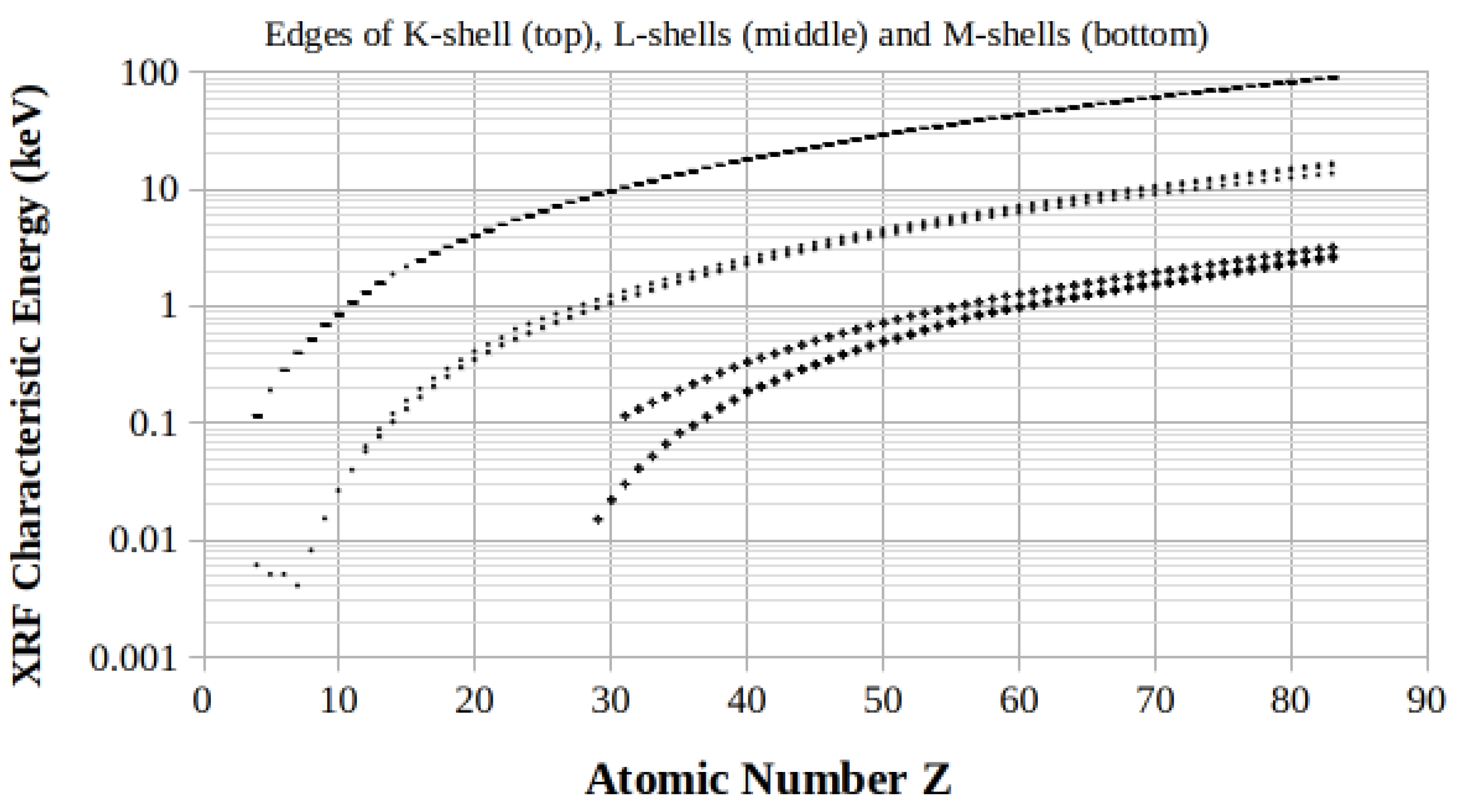
Figure 2.
CaF2 , GaO, CMSM and RCB footprints for 140.5 keV photon energy. The logarithmic scales are in counts (a.u.) for both the Compton profiles and the full-energy peaks, while they are in %wt for the elements abundances in the mixtures, respectively.
Figure 2.
CaF2 , GaO, CMSM and RCB footprints for 140.5 keV photon energy. The logarithmic scales are in counts (a.u.) for both the Compton profiles and the full-energy peaks, while they are in %wt for the elements abundances in the mixtures, respectively.
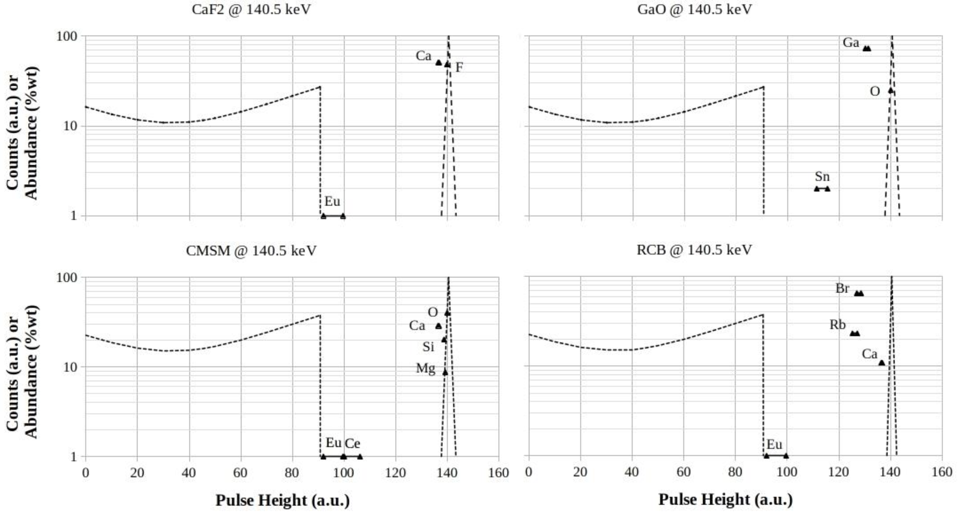
Figure 3.
YSO, NaI, CsI and LaCl footprints for 140.5 keV photon energy. The logarithmic scales are in counts (a.u.) for both the Compton profiles and the full-energy peaks, while they are in %wt for the elements abundances in the mixtures, respectively.
Figure 3.
YSO, NaI, CsI and LaCl footprints for 140.5 keV photon energy. The logarithmic scales are in counts (a.u.) for both the Compton profiles and the full-energy peaks, while they are in %wt for the elements abundances in the mixtures, respectively.
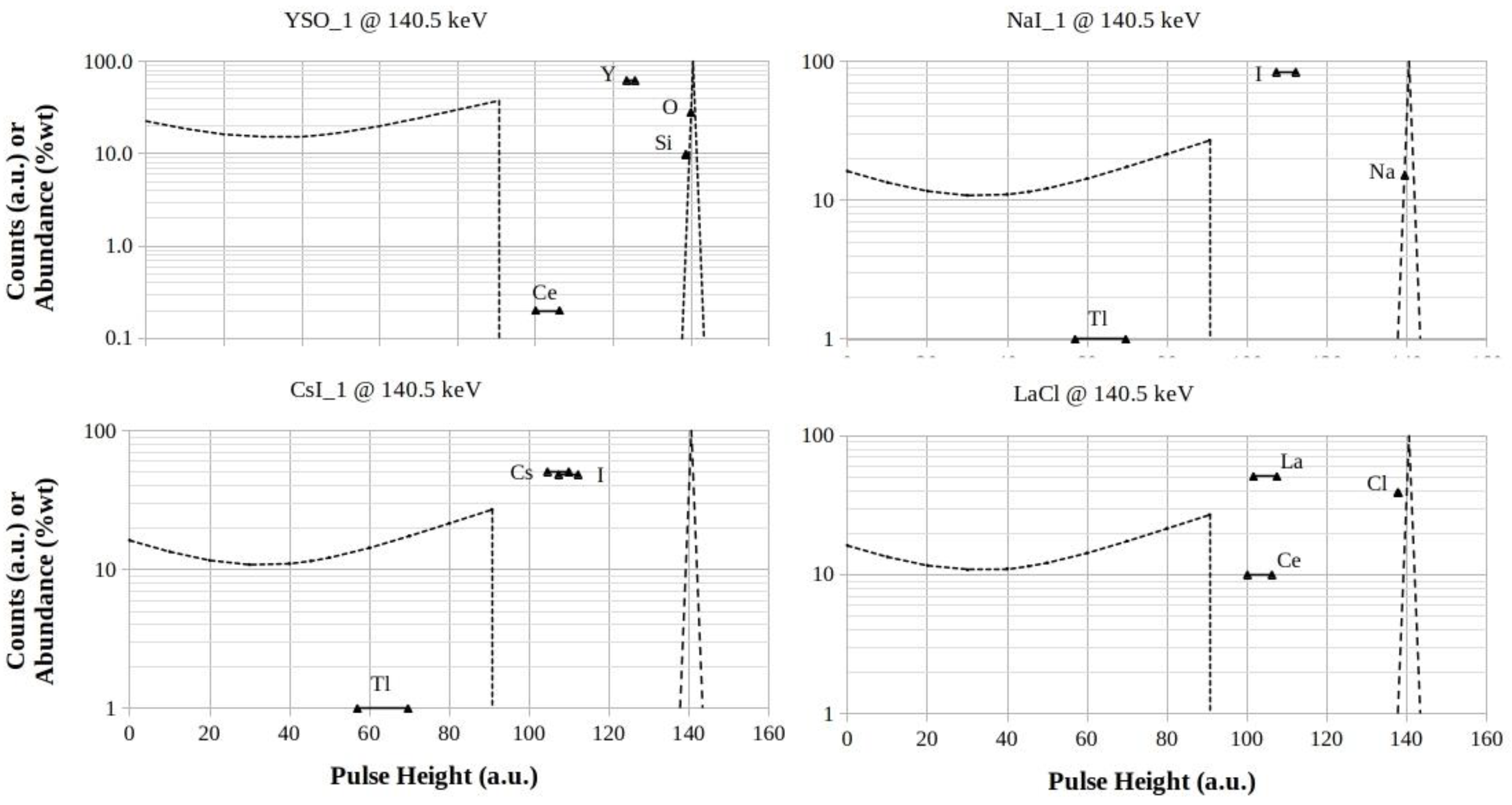
Figure 4.
GYAGG, CeF3 , LuYGAGG and LYSO footprints for 140.5 keV photon energy. The logarithmic scales are in counts (a.u.) for both the Compton profiles and the full-energy peaks, while they are in %wt for the elements abundances in the mixtures, respectively.
Figure 4.
GYAGG, CeF3 , LuYGAGG and LYSO footprints for 140.5 keV photon energy. The logarithmic scales are in counts (a.u.) for both the Compton profiles and the full-energy peaks, while they are in %wt for the elements abundances in the mixtures, respectively.
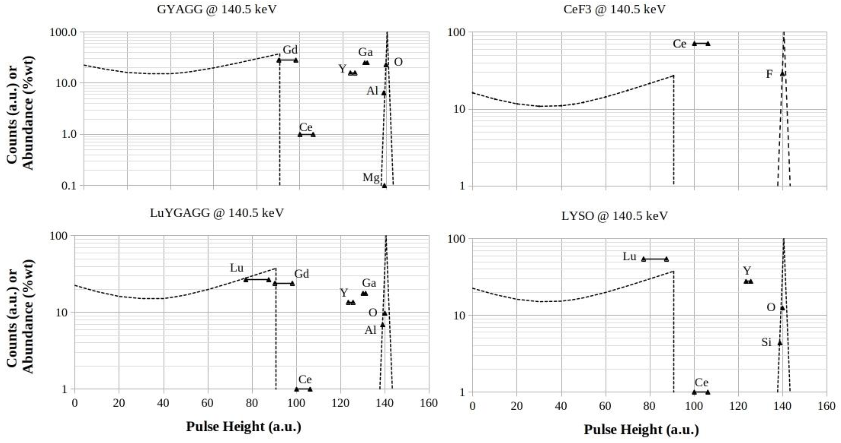
Figure 5.
LuYAP, LSO, LHO and BGO footprints for 140.5 keV photon energy. The logarithmic scales are in counts (a.u.) for both the Compton profiles and the full-energy peaks, while they are in %wt for the elements abundances in the mixtures, respectively.
Figure 5.
LuYAP, LSO, LHO and BGO footprints for 140.5 keV photon energy. The logarithmic scales are in counts (a.u.) for both the Compton profiles and the full-energy peaks, while they are in %wt for the elements abundances in the mixtures, respectively.
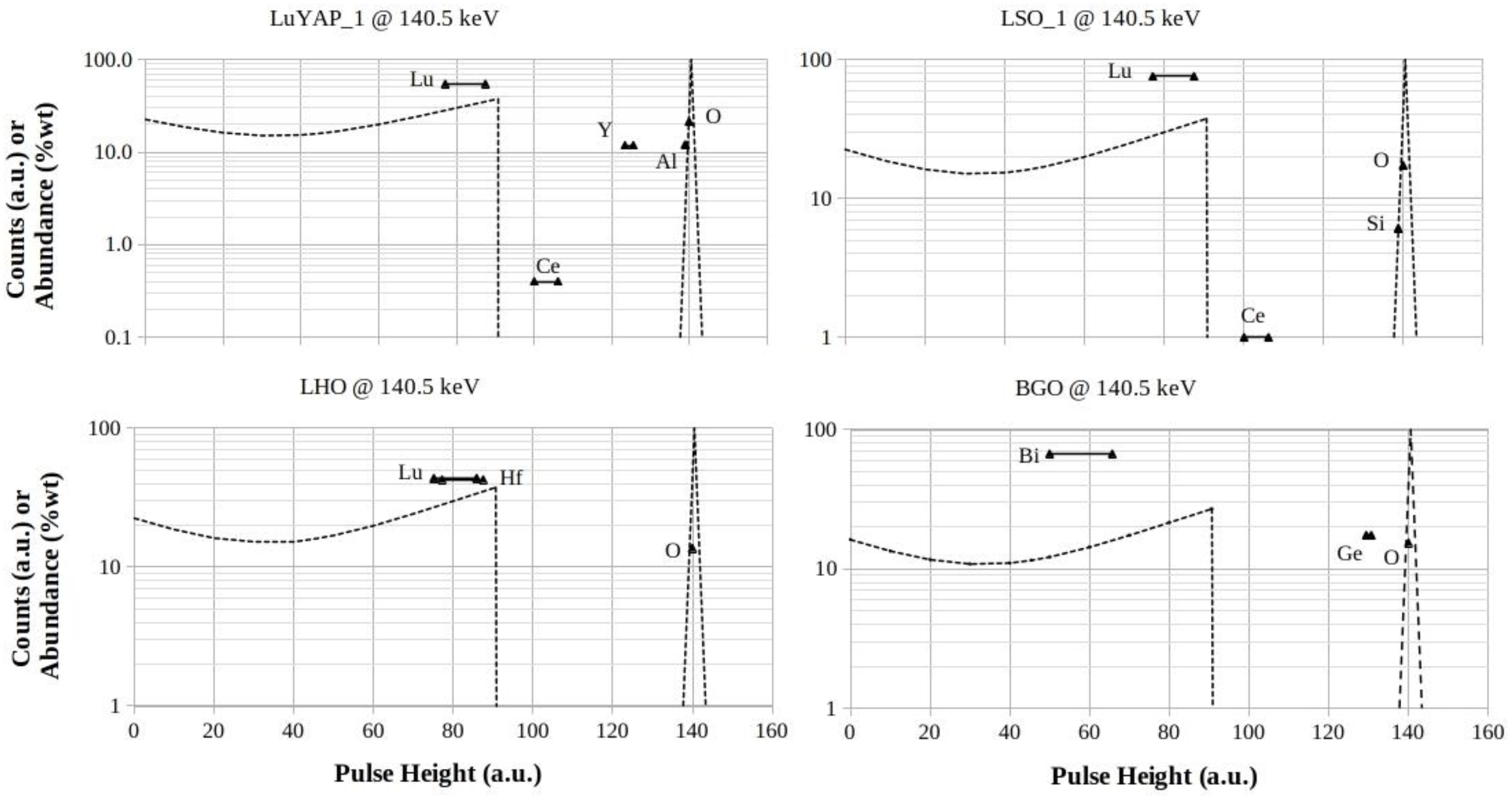
Figure 6.
CaF2 , GaO, CMSM and RCB footprints for 511 keV photon energy. The logarithmic scales are in counts (a.u.) for both the Compton profiles and the full-energy peaks, while they are in %wt for the elements abundances in the mixtures, respectively.
Figure 6.
CaF2 , GaO, CMSM and RCB footprints for 511 keV photon energy. The logarithmic scales are in counts (a.u.) for both the Compton profiles and the full-energy peaks, while they are in %wt for the elements abundances in the mixtures, respectively.
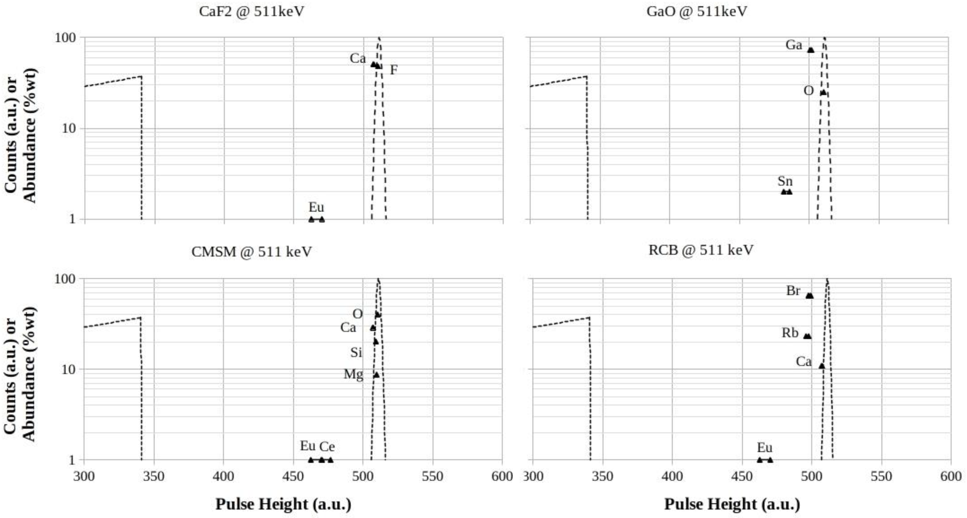
Figure 7.
YSO, NaI, CsI and LaCl footprints for 511 keV photon energy. The logarithmic scales are in counts (a.u.) for both the Compton profiles and the full-energy peaks, while they are in %wt for the elements abundances in the mixtures, respectively.
Figure 7.
YSO, NaI, CsI and LaCl footprints for 511 keV photon energy. The logarithmic scales are in counts (a.u.) for both the Compton profiles and the full-energy peaks, while they are in %wt for the elements abundances in the mixtures, respectively.
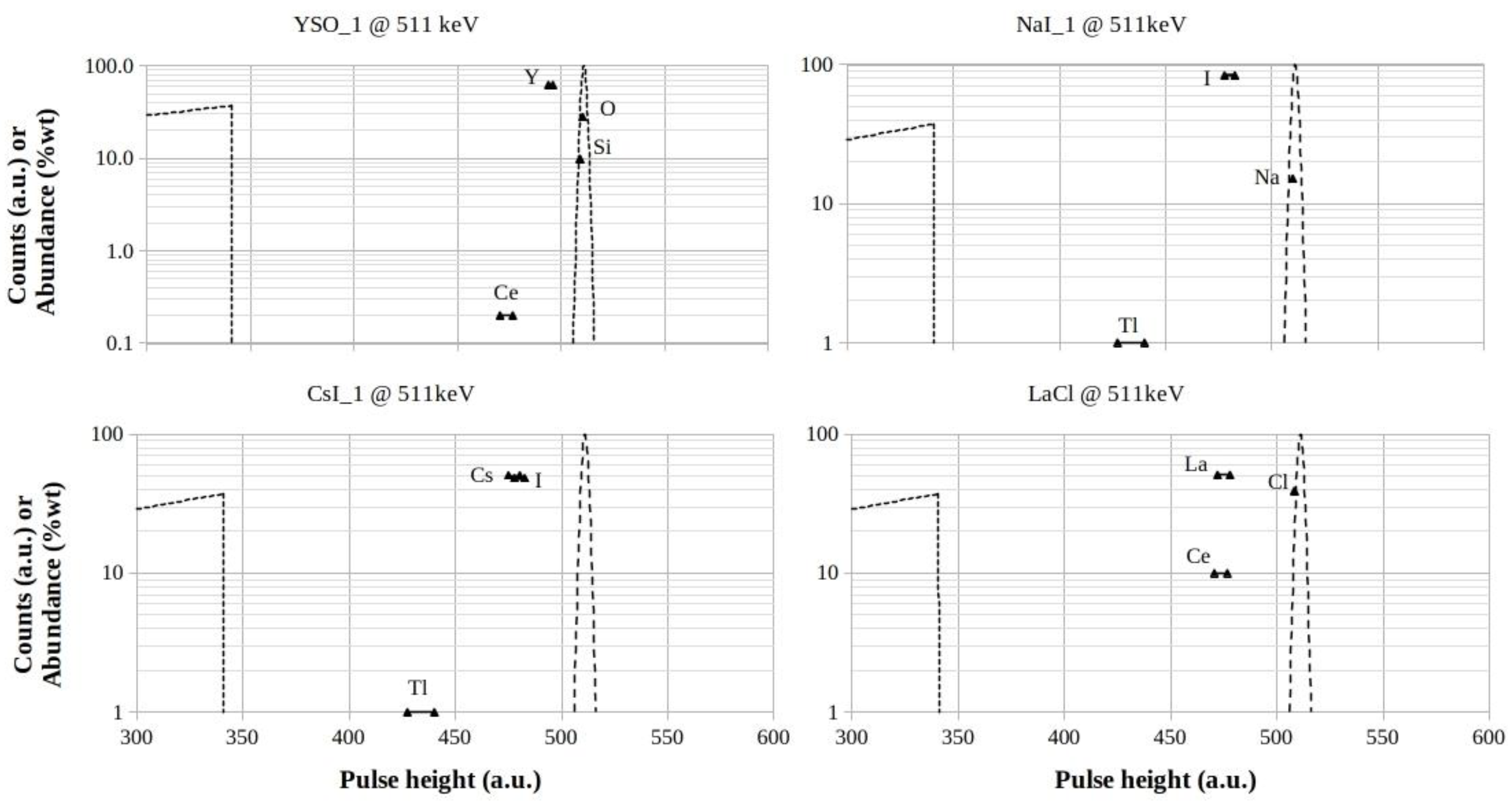
Figure 8.
GYAGG, CeF3 , LuYGAGG and LYSO footprints for 511 keV photon energy. The logarithmic scales are in counts (a.u.) for both the Compton profiles and the full-energy peaks, while they are in %wt for the elements abundances in the mixtures, respectively.
Figure 8.
GYAGG, CeF3 , LuYGAGG and LYSO footprints for 511 keV photon energy. The logarithmic scales are in counts (a.u.) for both the Compton profiles and the full-energy peaks, while they are in %wt for the elements abundances in the mixtures, respectively.
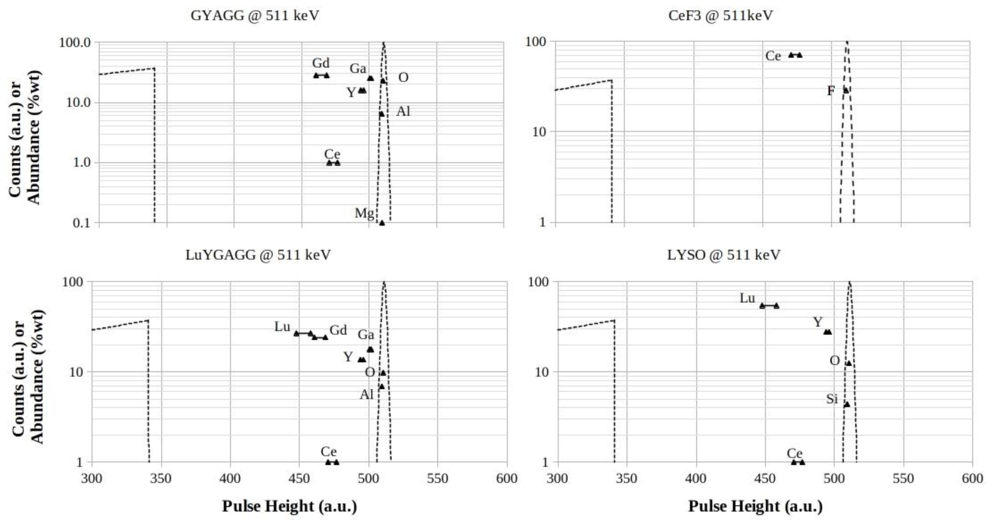
Figure 9.
LuYAP, LSO, LHO and BGO footprints for 511 keV photon energy. The logarithmic scales are in counts (a.u.) for both the Compton profiles and the full-energy peaks, while they are in %wt for the elements abundances in the mixtures, respectively.
Figure 9.
LuYAP, LSO, LHO and BGO footprints for 511 keV photon energy. The logarithmic scales are in counts (a.u.) for both the Compton profiles and the full-energy peaks, while they are in %wt for the elements abundances in the mixtures, respectively.
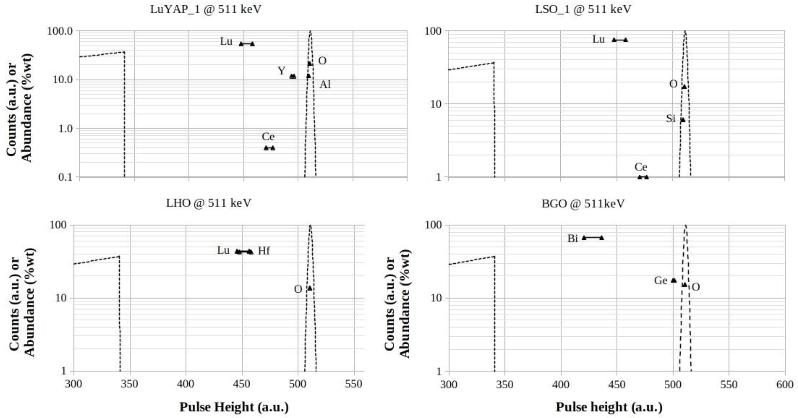
Figure 10.
CaF2 , GaO, CMSM and RCB footprints for 661.6 keV photon energy. The logarithmic scales are in counts (a.u.) for both the Compton profiles and the full-energy peaks, while they are in %wt for the elements abundances in the mixtures, respectively.
Figure 10.
CaF2 , GaO, CMSM and RCB footprints for 661.6 keV photon energy. The logarithmic scales are in counts (a.u.) for both the Compton profiles and the full-energy peaks, while they are in %wt for the elements abundances in the mixtures, respectively.
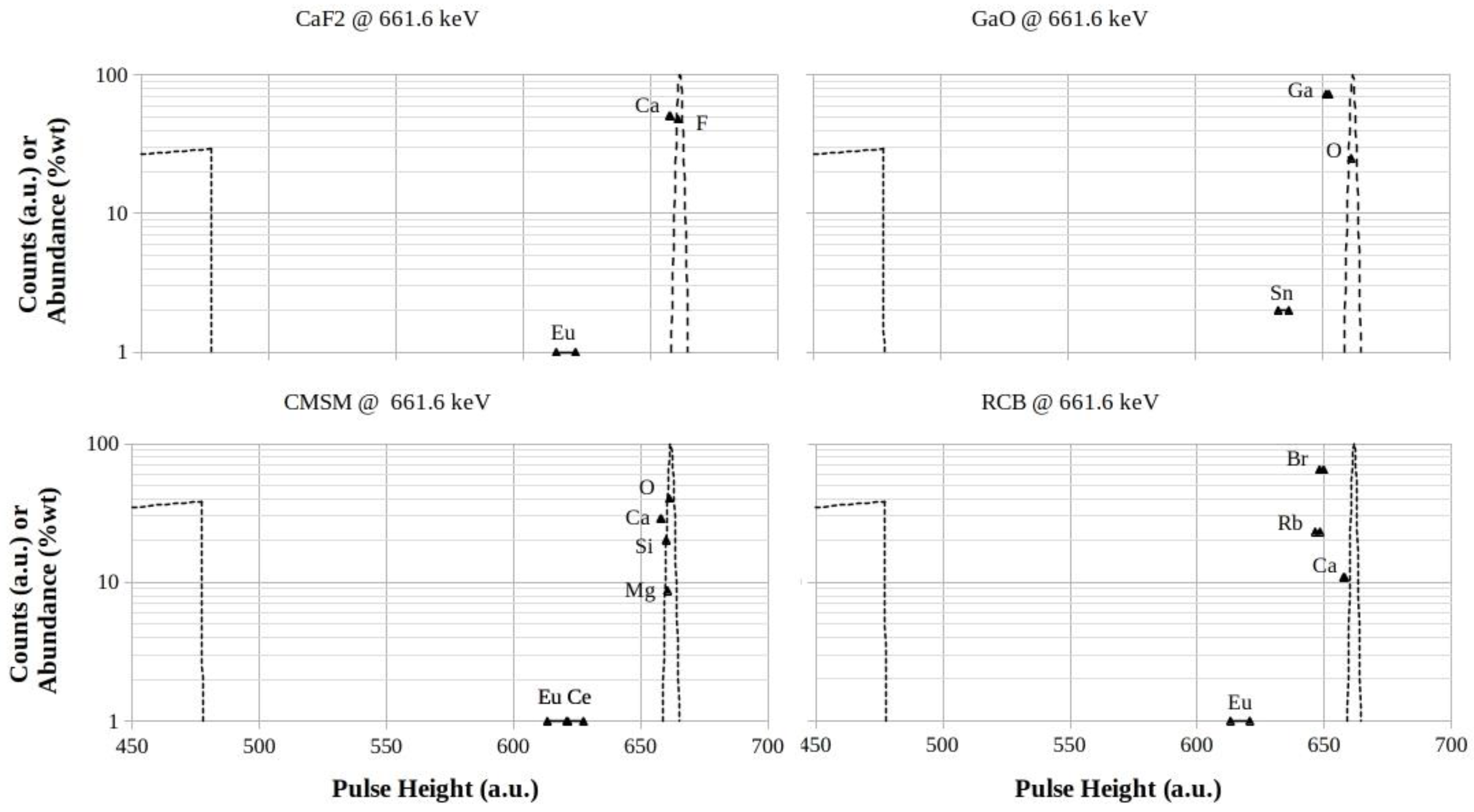
Figure 11.
YSO, NaI, CsI and LaCl footprints for 661.6 keV photon energy. The logarithmic scales are in counts (a.u.) for both the Compton profiles and the full-energy peaks, while they are in %wt for the elements abundances in the mixtures, respectively.
Figure 11.
YSO, NaI, CsI and LaCl footprints for 661.6 keV photon energy. The logarithmic scales are in counts (a.u.) for both the Compton profiles and the full-energy peaks, while they are in %wt for the elements abundances in the mixtures, respectively.
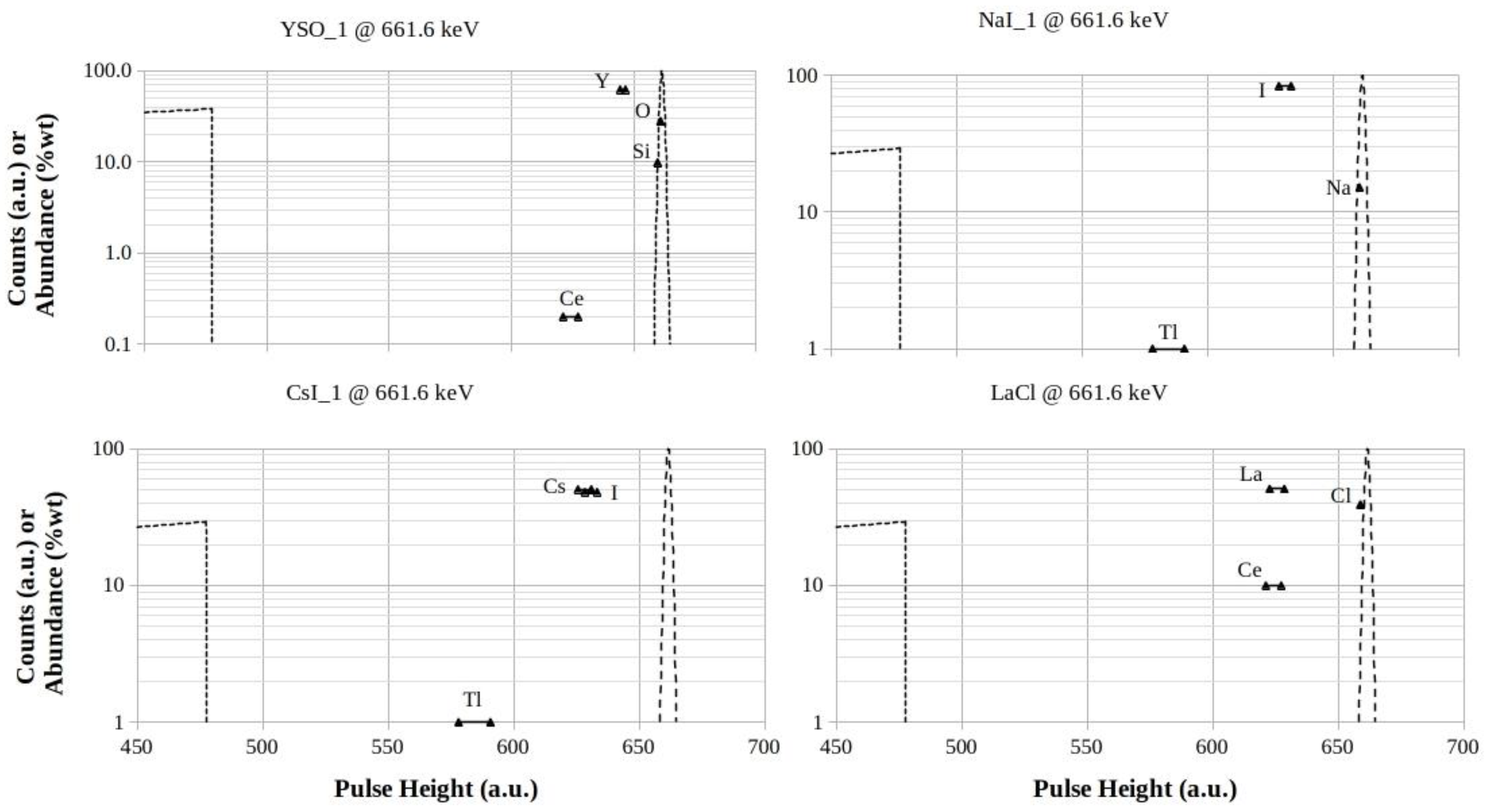
Figure 12.
GYAGG, CeF3 , LuYGAGG and LYSO footprints for 661.6 keV photon energy. The logarithmic scales are in counts (a.u.) for both the Compton profiles and the full-energy peaks, while they are in %wt for the elements abundances in the mixtures, respectively.
Figure 12.
GYAGG, CeF3 , LuYGAGG and LYSO footprints for 661.6 keV photon energy. The logarithmic scales are in counts (a.u.) for both the Compton profiles and the full-energy peaks, while they are in %wt for the elements abundances in the mixtures, respectively.
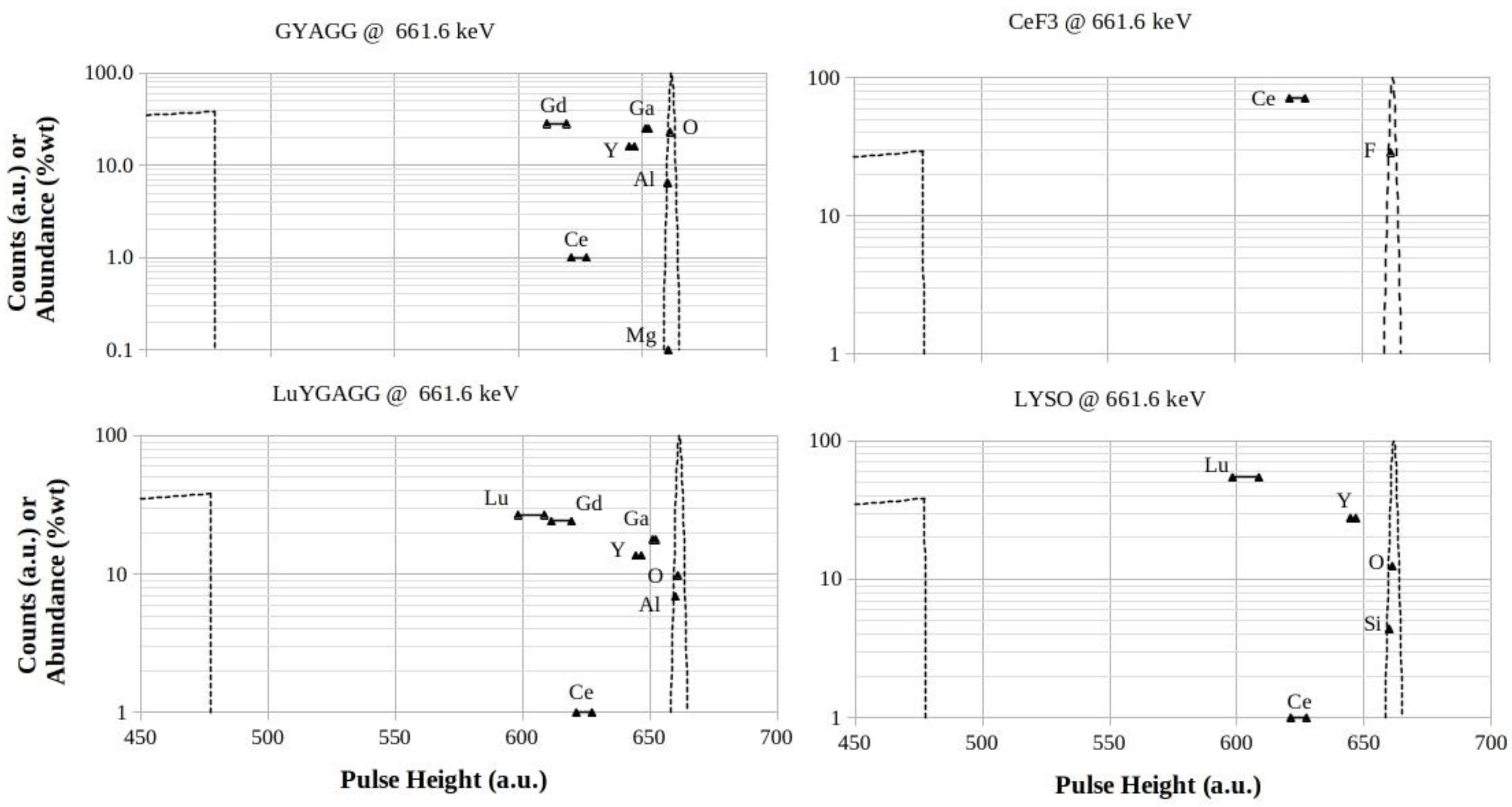
Figure 13.
LuYAP, LSO, LHO and BGO footprints for 661.6 keV photon energy. The logarithmic scales are in counts (a.u.) for both the Compton profiles and the full-energy peaks, while they are in %wt for the elements abundances in the mixtures, respectively.
Figure 13.
LuYAP, LSO, LHO and BGO footprints for 661.6 keV photon energy. The logarithmic scales are in counts (a.u.) for both the Compton profiles and the full-energy peaks, while they are in %wt for the elements abundances in the mixtures, respectively.

Disclaimer/Publisher’s Note: The statements, opinions and data contained in all publications are solely those of the individual author(s) and contributor(s) and not of MDPI and/or the editor(s). MDPI and/or the editor(s) disclaim responsibility for any injury to people or property resulting from any ideas, methods, instructions or products referred to in the content. |
© 2024 by the authors. Licensee MDPI, Basel, Switzerland. This article is an open access article distributed under the terms and conditions of the Creative Commons Attribution (CC BY) license (http://creativecommons.org/licenses/by/4.0/).
Copyright: This open access article is published under a Creative Commons CC BY 4.0 license, which permit the free download, distribution, and reuse, provided that the author and preprint are cited in any reuse.


