
Submitted:
13 December 2024
Posted:
16 December 2024
You are already at the latest version
Abstract
Holders of life insurance policies can exercise various options that lead to contract modifications, e.g.
full surrender, partial surrender, paid-up and dynamic premium increase options. Transitions between
these contract states materially affect (current and future) cash flows, and thus represent a serious
source of uncertainty for an insurance company. It is common practice to determining best estimate
assumptions for these transitions independently, i.e. without considering joint determinants of the
different aspects of policyholder behaviour. Our paper shows how consistent best estimate transition
rates for multiple status transitions can be derived using data science methods. More specifically,
we extend existing multivariate approaches with the Lasso method such that the key drivers for
each transition can be identified automatically. We discuss the performance, the complexity and the
practical applicability of the different modelling approaches based on data from a European insurer.
Keywords:
multistate
; multi-class
; lapse rate
; paid-up
; life insurance
; Lasso
1. Introduction
A crucial part in the risk management of a life insurance company is the proper modelling of future policyholder behaviour. Contract modifications for existing policies are an important part of this customer behaviour and there are several different legal and contractual options for the policyholder, e.g. full surrender, partial surrender, paid-up and dynamic premium increase options. The resulting various contract states and in particular the transition between states have a material impact on the cash flow profile of the insurance company. This poses a serious risk, as the cash flows have a direct impact on the asset liability management. Consequently, under the European regulatory framework Solvency II, all contractual options and the factors affecting the exercise of these options need to be taken into account in the best estimate valuation, and the risk related to all legal and contractual policyholder rights has to be assessed in a separate risk sub-module denoted as `lapse risk’ (see articles 32 and 142 in [9]). In practice, independent models for each policyholder option are built with the Whittaker-Henderson approach (a univariate smoothing algorithm), see for example SAV [28] or Generalised Linear Models (GLM), see for example Haberman and Renshaw [14]. However, modelling these risks separately can lead to false interpretations and bad management decisions. We therefore advocate for a holistic modelling of policyholder options that allows for a consistent prediction of future cash flows. Furthermore, the choice of the `correct’ variables for the Whittaker-Henderson approach and the GLM is both manual (and therefore subjective) and time-consuming, since a potential new covariate (or interaction) requires a full readjustment of the previously considered covariates.
In this paper, we show how holistic policyholder behaviour models can be set up efficiently. Of course, there are different multivariate modelling approaches with different levels of manual interventions. In particular, data analytics techniques such as the Lasso can be used to replace the manual process of variable selection with a data driven approach. This also enables us to compare the different multivariate modelling approaches objectively and fairly. The joint modelling approach also addresses modelling issues due to low data volume for policyholder options that are less frequently exercised.
Building a multi-state model for policyholder behaviour has two core dimensions of complexity. First, the overall model choice: Several approaches in the field of survival analysis, (generalised) linear models and other machine learning areas are available. We choose to focus on GLM based models using extended Lasso penalties. By that, we can model complex policyholder behaviour while retaining parsimony and interpretability. But even within the Lasso based models, there are numerous ways of allowing for multiple states. Second, the inclusion of the transition history to the model: There are different ways of including information about previous states of a life insurance contract, that may impact the probability of future transitions.
In actuarial literature, binary lapse behaviour for insurance companies has been analysed thoroughly. Most research focuses on macroeconomic variables (e.g. interest rate or unemployment rate) and analyses hypotheses like the interest rate hypotheses or the emerging fund hypothesis. See for example [18] for the German market. Due to the confidentiality of policyholder data, there is limited research on the effect of policy specific variables (e.g. contract duration or sum insured) on lapse behaviour. Refer to [8] for an overview of both macroeconomic and policy specific research on lapse in life insurance.
The main tools used to analyse lapse behaviour on a policyholder level are survival analysis, see e.g. [25], and Generalised Linear Models (GLM), see e.g. [3] and [7]. There are also machine learning approaches to analyse lapse behaviour. Refer to [27], [2] and [31] for an extended Lasso approach, a random forest or a neural network, and a support vector machine, respectively.
In these papers, lapse is the only state (besides active), meaning that the response is treated as a binary variable. Now we allow for more states and address multi-state policyholder behaviour (with lapse being one possible state). Modelling several states and transitions between these states is not an entirely new topic in actuarial science and was already discussed in [12]. In fact, this type of analysis is common in certain areas, especially in health insurance, e.g. with possible states active, disabled and dead. Of course, the specific states and possible transitions depend on the insurance product, see e.g. [4].
There are also some multi-state applications in life insurance: [32] uses a Markov process to model different fitness states (and transitions between them) and their effect on mortality. [21] analyse mortality rates for potentially changing states of socio-economic factors (e.g. income or smoking). [25] analyse lapse behaviour with multiple possible states using a competing risk approach (survival analysis). Finally, [5] analyse customer churn using a multinomial logistic regression (MLR) and a second-order Markov assumption. They also compare the MLR with a binary one-versus-all model, as well as a gradient boosting machine and a support vector machine.
In this paper, the actuarial literature is extended by the implementation of different modelling approaches based on extended versions of the Lasso. This includes a discussion of the architecture of the different approaches, the corresponding aggregation schemes applied to get the overall predictions, and different orders of the Markov assumption. We compare the different modelling approaches and Markov assumptions quantitatively and qualitatively.
The remainder of this paper is organised as follows: In Section 2, we introduce different modelling approaches for the underlying multi-state problem and discuss qualitative features of each approach. We also present different ways of including the transition history in each modelling approach. Section 3 introduces the data set and other details of the implementation. It supplements the previous section by adding quantitative aspects of the different modelling approaches. In Section 4, we show the numerical results, and compare the different modelling approaches and the different ways of including the transition history. Finally, Section 5 concludes.
2. Modelling Multiple Status Transitions
In this section, we present different approaches for modelling multiple status transitions and focus on qualitative aspects for the model selection: we differentiate with respect to structure, uniqueness, complexity of the model, and the possibility to generalise to an arbitrary number of transitions. We also analyse and compare approaches to consider the history of an insurance contract in a model. This section focuses on the architecture for the different modelling approaches, while the specific implementation and application for our data set is described in Section 3 and compared in Section 4.
In our analysis of a typical insurance portfolio, only annual status transitions are tracked. Therefore, the initial status at the beginning of a year and the status at the end of the year is recorded and exactly one potential transition during the year can be further analysed and considered in a multi-class problem. In the literature, there are several model structures for multi-class response variables where an estimated probability for each potential class is derived, and there are basically two ways of modelling such a multi-class problem: Firstly, decomposition strategies transform the original multi-class problem into several binary problems and subsequently combine them to get a multi-class model. Those approaches are particularly interesting for machine learning models like support vector machines which were originally designed for binary problems. In the GLM framework, the binary model corresponds to a logistic regression. An overview for decomposition strategies is given in [23]. The decomposition strategies used for this analysis are described and discussed in SubSection 2.1 - Section 2.3. Secondly, models with a holistic strategy can handle multiple classes directly with no need for a decomposition. In the GLM framework, this corresponds to a MLR as described in [10]. This approach is described in SubSection 2.4.
In the analysis of policyholder behaviour, the transition history may impact future transition probabilities, e.g. the lapse probability may be increased for a contract that was made paid-up recently compared to a contract that has been paid-up for a longer time. Therefore, different approaches of including the history to the model are discussed in SubSection 2.5. These approaches can be applied for both the decomposition approaches and the holistic approach.
For recurring terms, we use the notation:
- K is the set of possible classes for the response variable Y with potential classes.
- Based on [1], M corresponds to a coding matrix with possible entries . Each column j corresponds to a binary base model, indicating whether the class (in row i) has a positive label (), has a negative label () or is not included (). The latter means that data from class i is not reflected in the calibration of model j.
- describes the (predicted) probability that an observation x is in the subset of classes I.
- denotes the subset of the observations, where .
- .
- In general, p describes a (predicted) probability from a binary model, i.e. before aggregation, and q describes a (predicted) probability for a multi-class model, i.e. after aggregation.
Hypothetical example: We illustrate each model with a hypothetical data set with three classes ( and ) for the response variable and two not further specified covariates and (adopted from [33]), see Figure 1. Each observation in this example is depicted in the two-dimensional plane (covariates) where each class (response) is visualised by a different colour and symbol.
2.1. One vs. All Model
The one vs. all (OVA) model (also called one against all (OAA)) is a popular choice among the decomposition strategies. As the name suggests, the OVA approach builds several binary models, where each models one class versus all the other classes:
Figure 2 shows the model architecture for the hypothetical example. The black lines represent binary model results separating the two relevant classes using the two covariates.
An aggregation scheme is necessary to transform the probabilities from the binary models into a multinomial model with probabilities for each class1. Note that the models themselves are unbiased, in the sense that the average predicted value equals the average observed value. Therefore, the average predicted values of the individual models add up to one. However, this is not necessarily valid for a single observation and in general, the sum of the predicted probabilities is not equal to one here. An intuitive approach for the aggregation is a rescaling of the individual probabilities, such that the original ratios are conserved, but the probabilities also add up to one for each single observation:
This aggregation scheme is also statistically motivated, since the rescaled probabilities are closest (in terms of Kullback-Leibler distance, see [20]) to the individual probabilities , while adding up to one:
There are also other possible aggregation schemes.
For the OVA model with the rescaling aggregation scheme, there are m binary models that have a unique definition and are independent from each other. However, the aggregation scheme implies a dependency for the actual target q. Thus, a prediction for a specific class may impact or even worsen the predictions for other classes.
2.2. One vs. One Model
The one vs. one (OVO) model (also called one against one (OAO)) is another popular choice among the decomposition strategies. As the name suggests, the OVO approach builds several binary models, where each models one class versus another class:
Figure 3 shows the model architecture for the hypothetical example. Again, an aggregation scheme is necessary to obtain a multinomial model with probabilities for each class2. There are several possibilities on how to aggregate the probabilities from the individual binary models in order to estimate the probability distribution of the underlying data set , see e.g. [11]. Also note that the individual models in the OVO approach can `contradict’ each other in the sense, that there is no compatible set of probabilities , e.g. if and .
In this analysis, we apply pairwise coupling as proposed by [16] for the aggregation. The idea is to minimise the (weighted) sum of the Kullback-Leibler distances between and , where the weights correspond to the number of observations in :
For the example above, where and , the proposed aggregation scheme (with ) gives and . Since the individual models would imply that A is more likely than B, B is more likely than C, but then C is more likely than A, the aggregated probabilities around seem reasonable. The order appears plausible as well since the combined estimated probabilities from the individual models are for classes and B.
An alternative and intuitive aggregation scheme for the OVO approach is the rescaling of the combined estimated probabilities such that the resulting probabilities add up to one. In the example above, this would lead to and . Even though the resulting probabilities (for this example) are very similar to those from the pairwise coupling, the alternative aggregation scheme performed significantly worse in the comparisons as laid out in Section 4. Therefore, we decided to omit this alternative aggregation scheme and focus on the pairwise coupling, even though the interpretability of the OVO approach suffers from the rather complicated aggregation scheme.
The number of necessary binary models increases rapidly with the cardinality of K. In general, there are models in case of m classes for the response variable and the individual models are independent for the sub-samples. As for the OVA, the aggregation scheme implies a dependency for the actual target q.
2.3. Nested Model
Nested models (also called hierarchical models) are another example for combining binary models to arrive at a multinomial model. OVA and OVO are symmetric in the sense that changing the order of the classes does not impact the result, i.e. these models have one unique definition. Within the nested approach, there are multiple ways of defining the hierarchical model setup. For example, in case of three classes, there are three possible model architectures:
Figure 4 shows the first model architecture (Nested A) for the hypothetical example.
In general, there are many separation possibilities, see Equation 1 below. In each step of the hierarchy, the remaining classes are split into two (potentially imbalanced) parts until finally, each class is separated. Therefore, each individual class k has subsets describing the unique separation path of length s: .
The hierarchical design of the aggregation scheme ensures well defined probabilities, and thus an aggregation scheme is not necessary for the nested approaches. To obtain the prediction of a class, we use the specific path for that class:
The specific order is rather arbitrary and has a major impact on the complexity of the prediction . We will see in Section 3 that this order also affects the quality of the model fit tremendously. This dependency on the order is a major disadvantage of the nested models. In some applications, expert judgement can help to identify a reasonable order. In many applications, however, the best possible order is a-priori unknown.
In general, there are models in case of m classes for the response variable, as for the OVO approach. However, this time the order matters. The models are not independent, since in each step of the hierarchy, the models condition on the result of the higher levels of the hierarchy. We have seen in the hypothetical example that for three classes only three different orders are possible. But with four classes there are 15 possible orders and with five classes already 105. To obtain a general formula for the number of possible orders, we derived a recursive formula based on combinatorial terms and then transformed it into the following compact representation using the Gamma-function:
where is the number of possible orders for m final classes.
Thus, there is potentially a huge number of possible model specifications and a high complexity introduced by the number of binary models.
2.4. Multinomial model
Instead of decomposing the multi-class problem into several binary problems (e.g. using the OVA, OVO or nested method), we can also approach the multinomial problem directly. Within the GLM framework, the most intuitive way is to use a MLR which is a direct generalisation of the logistic regression, see e.g. [10]. Figure 5 shows the model architecture for the hypothetical example. Also, outside of the GLM framework, there are several algorithms capable of modelling multiple classes, e.g. neural networks with softmax layer or random forests.
The MLR estimates all probabilities simultaneously. Therefore, we do not need to transform individual probabilities by an aggregation scheme as before. The black line in Figure 5 represents a hypothetical model to separate the classes - this time three classes simultaneously, instead of just two classes at a time.
This approach only uses one model, no matter how many states the response variable has. Hence it uses all information simultaneously for the prediction of an observation. The model structure is unique; therefore the model imposes a significant complexity reduction.
2.5. Transition History
There are many applications - including ours - where observations are made over time. In our data set (see Section 3.1), this corresponds to a yearly observation for each in-force contract. At the end of each complete contract year, the current state is tracked (which can be active, paid-up or lapse). Therefore, we do not differentiate between, for example, lapse after 4.5 contract years or 4.8 contract years. The remaining covariates do not change over time. This results in a sequence of possible states and transitions for each observation. The transition history of an observation may impact the probabilities of future transitions, e.g. the lapse probability may be increased for a contract that was made paid-up recently compared to a contract that has been paid-up for a longer time. In order to improve estimates of transition probabilities, it may be useful to consider the past of an observation in the model. There are several ways of including the transition history in the model and we focus on the following three approaches:
- No previous information: There is always the possibility to ignore any information about previous states. This is the easiest and most primitive way of dealing with the transition history but can still be legitimate for applications where the history is obviously irrelevant.
- Markov property: A Markov property can be assumed, see [6]. The `past’ (transition history) does not matter for the `future’ (predictions), given that the `present’ (current state) is known, i.e.:where t indicates the time (=contract duration) of an observation and corresponds to the state (active, paid-up or lapse) in that year t. Hence, we are modelling yearly lapse and paid-up rates.
- Full transition history: There are also applications in which it is possible to define one new covariate (or more), which represents the state history sufficiently. This highly depends on the number of states and the structure and dependencies of the underlying data set. In our specific example, the time since being paid-up seems to sufficiently describe the state history, see Section 3.1 for details.
In the second and third approach, there is still flexibility of how to include the information in the model. Let the status history be sufficiently described in one (or more) new covariate . Subsequently, it can be treated as a normal covariate in the model. Alternatively, the covariate and all its interactions with the remaining covariates can be included in the model. This allows the model to identify more complex structures in the data. A third way is splitting the data according to that covariate and building separate models for each subset. Note that this increases the number of individual models for each model architecture. Including the covariate to the model formula is no longer necessary since it is just constant for each subset. However, in cases where the history can only be captured sufficiently by many new covariates or if the number of possible classes is high this third approach may not be feasible. All above-mentioned approaches are analysed for our data set in Section 4.
3. Application for a European Life Insurer
In this section, we further specify, apply and compare the approaches for modelling multiple status transitions for a portfolio of life insurance contracts provided by a pan-European Insurer operating in four countries. An elaborate description of the considered models can be found in [24] for GLMs, in [29] for the Lasso, in [30] for the fused Lasso and in [19] for the trend filtering. Also see [27] for the application of the extended versions of the Lasso to a logistic lapse model.
3.1. Data Description
The data set contains a large number of insurance contracts over an observation period of around 21 years. This particular portfolio went into run-off after about 11 years, which means that no new contracts were written after that. However, this does not affect the proposed modelling approaches - they can also be applied to portfolios that are not in run-off.
Life insurance contracts typically include several options available to policyholders, such as full surrender (lapse) and stop of regular premium payments (paid-up), but also the option of reinstatement of premium payments after being paid-up, partial surrender, pre-defined dynamic premium increases and other premium increases, or payment of top-up premiums. For the contracts in this particular portfolio, the key observed status transitions of the contracts are the option of making a contract paid-up and the exercise of a full surrender (lapse) option. Thus, the data set appears well suited to apply the presented models using three possible states: active (A), paid-up (P), lapse (L). Note that for other portfolios significantly more transitions may need to be modelled.
In this paper, the option to `lapse’ is defined to comprise surrender (policyholder cancels the contract and gets the surrender value), pure lapse (insurance contract is terminated without a surrender value payment) and transfer (policyholder cancels the contract and transfers the surrender value to another insurance company). The second option `paid-up’ is defined by a reduction of regular premium payments to zero but the contract remains in force. Obviously, an execution of the first option implies a transition to a terminal status. The paid-up option leaves a potential lapse option for the future open.
There are observations ( unique contracts) with an extended set of up to covariates: contract duration (number of years between inception and observation time), insurance type (traditional or unit-linked), country (four European countries), gender, payment frequency (e.g. monthly or annually), payment method (e.g. debit advice or depositor), nationality (whether or not the country, in which the insurance was sold equals the nationality of the policyholder), dynamic premium increase percentage, entry age, original term of the contract, premium payment duration, sum insured and yearly premium. We extend this original set of covariates by including two covariates that contain information about the previous state(s) of a policyholder. For some models, we only consider the previous status (i.e. active or paid-up, since lapse is the terminal status). For other models, we also add another covariate: time since paid-up which counts the years between being made paid-up and the observation time. It is defined as 0 as long as a policyholder is still active (of course, each policyholder initially starts in the active state). For this data set, there are no observations with reinstatement, meaning that we do not observe the transition P → A. Other covariates do not change over time and are therefore deterministic for our life insurance portfolio. Hence, the covariates contract duration and time since paid-up uniquely determine the full state history of a contract3.
For modelling purposes, a separate row is created for each in-force contract in each observation year. As a consequence, one single contract may occur in several rows in the data set - once for each observation year where the contract is still in force. This differs from a standard survival analysis setup, where we would typically have one observation per contract. This observation would then contain information about the duration (until being paid-up and until lapsing), a potential censoring and the final state. This modification leads to a data set where the rows are no longer fully independent, and we also have a selection bias (contracts being in-force longer get more weight than contracts lapsing early). Given the size of our data set, this modification seems justifiable. However, in general, the effect of this modelling approach should be analysed carefully.
Figure 6 shows the decreasing exposure (upper part) and the composition of the three states (lower part) for different values of contract duration. The one-year lapse rates clearly decrease rapidly in the first three years which is consistent with the well-known higher lapse rate at the beginning of an insurance contract. The one-year paid-up rate shows a different trend: starting with a very small percentage for the first year of the contract, the rate increases over time until it reaches a certain threshold. Although the rates have different trends, they should be modelled consistently together.
One useful pre-processing step in this framework is the binning of continuous covariates. By that, the corresponding covariate has several pre-defined category levels (bins). Without binning, the model can either estimate a single parameter for the continuous covariate (and potentially underfit) or estimate a parameter for every single value of the covariate by treating it as a factor (and potentially overfit). With binning, we are therefore able to derive an interpretable model with a good predictive power to satisfy the requirements of an insurance company.
There are different possibilities for choosing adequate bins, e.g. bucket binning (each bin has the same length), quantile binning (each bin has the same number of observations) or simply relying on expert knowledge. There are also more complex ways of defining bins: [17] use evolutionary trees as described in [13] to estimate optimal bins for continuous variables. These evolutionary trees incorporate genetic algorithms to the classical tree framework to find the global optimum by allowing changes also in previous splits. We choose a rather simple data-driven approach (no expert knowledge) to derive the bins and follow the approach of [27] using a univariate decision tree for each continuous covariate in the data set: entry age, original term of the contract, premium payment duration, sum insured and yearly premium. To avoid overfitting, we use small trees with at least 5% of the observations in each terminal leaf (see again [27]). Note that contract duration is not assumed to be continuous, and no univariate decision tree is built. The category levels are therefore just the natural numbers up to 20.
3.2. General Model Setup
Since we are looking for a parsimonious and interpretable model, we focus on GLM based models using extended versions of the Lasso in our analysis. The probabilities are defined as:
The first equation corresponds to the logistic regression (binary case of the decomposition strategies) and the second equation corresponds to the MLR with m classes. The logistic regression is a special case of the MLR with . However, in Equation 2 the reference level for the logistic regression is implicitly set to one of the two classes, while there is no explicit reference level for the MLR. Consequently, we only consider those coefficients not corresponding to class A in the results Table 3 to make the comparison of the number of coefficients in the models fair.
For the logistic regression, we have the following log-likelihood function:
The parameters are estimated with a penalised maximum likelihood optimisation (regularisation). We use the methodology proposed by [27]:
where represents different versions of the Lasso, i.e. regular Lasso, fused Lasso and trend filtering. The regular Lasso penalises the difference of each category level to the intercept () and can be used for covariates without ordinal scale. The fused Lasso penalises the difference between two adjacent category levels () and is therefore suitable for fusing neighbouring category levels. Finally, the trend filtering penalises the difference in linear trend between category levels (). It is hence used for modelling a piecewise linear and often monotone structure within that covariate.
For the MLR, the equations can be adjusted according to:
and
These extended versions of the Lasso allow the model to capture structures within covariates - however only for the effect on a specific value of the response variable. A penalisation across different values of the response variable is not possible in this modelling setup. For example, two different coefficients for the effect of a covariate j on lapse and may be fused together. Similarly, the two different coefficients for the effect of covariate j on paid-up and may be fused together. However, a fusing between and or between and is not possible. To our knowledge, this form of optimisation has not been implemented yet.
For the implementation, we essentially use the same setup as described in [27], which can be summarised by
- modelling the trend and fused Lasso penalty with contrast matrices, and
- determining the hyper-parameter based on a 5-fold cross-validation using the one standard error (1-se) rule.
3.3. Specific Model Setup and Parameter Estimation
For the decomposition strategies, Equation 3 can be applied for each binary model independently, based on the coding matrices M. This results in the calibration of three independent binary models, see and , or two independent binary models, see and . Therefore, we perform three (two) independent penalised maximum likelihood estimations using Equation 3 with corresponding and . The calibration of the binary models is independent and therefore the values of penalisation terms differ in general, see Table 1. In contrast, the MLR only requires a single model calibration using Equation 4.
The table shows some main findings:
- The second model of each nested approach is identical to a model in the OVO approach. Of course, this can also be seen when comparing the columns of in Section 2.2 with and in Section 2.3.
- Splitting the data set requires an additional model which is identical for all approaches (cf. last entry in the last column). For the subset with initial state `active’, the number of models is identical to the previous number of models (including both initial states), because the corresponding response variable can still have all three states `active’, `paid-up’ and `lapse’. For the subset with initial state `paid-up’ however, one additional model is required with possible levels `paid-up’ and `lapse’ for the response variable. It is just a single logistic regression with initial state ’paid-up’ and response ’paid-up’ or ’lapse’.
- Whenever a model distinguishes class P from one (or all) other classes, the corresponding value is rather high - especially when comparing P and L (see e.g. Nested A, second model). A plausible interpretation might be that separating class P is comparably easy for a model in the sense that the model performance does not decrease when the penalisation is increased.
- The decomposition strategies have a higher degree of freedom in terms of value, because they might differ for the individual binary models. In this application, however, the values seem to have a similar magnitude across the different modelling approaches. Note that we also optimised the penalised likelihood functions from the decomposition strategies with the restriction of a constant penalisation term for all binary models. As expected, the impact on the results was rather small. This might be different in applications where the independently calibrated values vary more. In the end, we chose the penalisation terms of Table 1, which is consistent with the independent model definitions.
In principle, may also differ for the individual binary models within a decomposition strategy. This again leads to a high degree of flexibility, e.g. if and . However, this flexibility did not seem to impact the result significantly, such that we chose the same penalty type for all models, as described in Table 2 and in line with [27].
Finally, the estimated coefficients are fed into Equation 2. For the decomposition strategies, the resulting probabilities are then transformed using the aggregation schemes presented in Section 2. For the MLR, the resulting probabilities are directly well defined and do not require further modifications.
4. Results and Comparison of the Modelling Approaches
After we have described the different modelling approaches as well as the calibration to the underlying data set, we now analyse and compare the results. We focus on two dimensions: the different model architectures (see Section 2.1 - Section 2.4) and the inclusion of the transition history (see Section 2.5). We have seen that due to their architecture, some of the models require a considerable effort and readjustment to generate multinomial probabilities. Therefore, we also include the complexity (number of models and number of parameters) and the computing time of the models as additional components that are obviously important for the model selection.
Table 3 shows the two dimensions of the analysis: The rows show different model architectures, and the columns show different ways of including the transition history. Note that we may also consider other dimensions in a sensitivity analysis, like for example different penalty types (regular, fused and trend), values, regularisation types (ridge, elastic net) or binning techniques. We would expect similar results as in [27].
The table is split into three parts: The upper part shows the performance of the models. The performance measure is defined as , where corresponds to the deviance of the model and corresponds to the deviance of the intercept only model (or null model). Therefore, it can be interpreted as the relative improvement over the intercept only model. This measure is similar to the measure for normally distributed response variables, with a similar interpretation. Since the measure is based on the deviance, it is also consistent with the likelihood optimisation described in Section 3.2. Other performance measures (e.g. the multi-class area under the curve (AUC) as defined by Hand and Till [15]) show a similar pattern. The middle part of the table shows the number of models, the number of parameters and the number of potential parameters. An entry thus means, that a individual models were built to get the overall prediction, a total of b parameters were selected by the underlying Lasso out of c possible parameters from the underlying dataset(s). Parameters where the Lasso assigns a value of zero are not included in this entry b as they implicitly disappear from the model. The lower part of the table shows the computing time (in minutes) on a standard computer. The aggregation scheme for the OVA model is very simple, so there is no measurable effort here. For the OVO model, however, the aggregation effort is considerable. For this model, the aggregation effort is given in parentheses.

Table 3.
Comparison of the different modelling types and transition histories, showing a performance measure based on the deviance (upper part), the number of models and parameters (middle part) and the computing time (lower part).
Table 3.
Comparison of the different modelling types and transition histories, showing a performance measure based on the deviance (upper part), the number of models and parameters (middle part) and the computing time (lower part).
| Markov property | |||||
|---|---|---|---|---|---|
| Model |
no previous information |
Markov property |
full transition history |
including interactions |
splitting the data set |
| Improvement over intercept only model: [in %] | |||||
| Intercept only | 0.0 | 0.0 | 0.0 | 0.0 | 0.0 |
| OVA | 37.6 | 48.4 | 48.5 | 50.0 | 49.9 |
| OVO | 39.9 | 50.8 | 50.9 | 51.4 | 51.3 |
| Nested A | 30.0 | 46.6 | 46.7 | 47.4 | 47.3 |
| Nested P | 37.9 | 48.2 | 48.5 | 50.4 | 50.2 |
| Nested L | 42.5 | 50.1 | 50.1 | 50.9 | 50.8 |
| MLR | 37.9 | 48.2 | 48.6 | 50.4 | 50.3 |
| Number of models, parameters and potential parameters | |||||
| Intercept only | 1/1 | 1/1 | 1/1 | 1/1 | 1/1 |
| OVA | 3/179/225 | 3/170/228 | 3/212/276 | 3/276/447 | 4/162/298 |
| OVO | 3/159/225 | 3/148/228 | 3/191/274 | 3/199/447 | 4/160/298 |
| Nested A | 2/104/150 | 2/108/152 | 2/134/184 | 2/154/298 | 3/126/223 |
| Nested P | 2/122/150 | 2/107/152 | 2/134/182 | 2/161/298 | 3/101/223 |
| Nested L | 2/112/150 | 2/103/152 | 2/135/184 | 2/160/298 | 3/113/223 |
| MLR | 1/94/150 | 1/86/152 | 1/108/184 | 1/171/298 | 2/104/223 |
| Computing time [in minutes] | |||||
| Intercept only | 0 | 0 | 0 | 0 | 0 |
| OVA | 8 | 12 | 13 | 16 | 8 |
| OVO | 7 (138) | 8 (140) | 8 (136) | 9 (136) | 5 (95) |
| Nested A | 5 | 5 | 6 | 7 | 3 |
| Nested P | 6 | 7 | 7 | 10 | 6 |
| Nested L | 7 | 7 | 8 | 10 | 5 |
| MLR | 14 | 16 | 17 | 26 | 10 |
Figure 7 visualises a part of the information from Table 3. The different models (except the intercept only model) are visualised by colours and the different transition histories are visualised by shapes. The x-axis shows the number of parameters, and the y-axis shows the relative improvement over the intercept only model.
4.1. Transition History
Markov property (vs. no previous information): We can clearly see in the figure (or in the Markov property column) that the previous state contains valuable information. All models perform significantly better with the previous state compared to the corresponding model without any previous information (between 8 and 17 percentage points). This is intuitive since the fact that a contract was already paid-up before impacts the chance of being paid-up in the current year. Since only one potential coefficient is added to the model (), the number of parameters does not change a lot (all changes within plus and minus 15%) and for most of the models even decreases, e.g. from 112 to 103 for Nested L. This is an indicator that the additional covariate contains valuable information such that other covariates are then no longer required in the model. Of course, this highlights one of the major advantages of using the Lasso approach: it selects the covariates automatically.
Full transition history (vs. Markov property): The full transition history including the time since being paid-up does not seem to improve the model significantly. Even though it increases the number of parameters (e.g. by 31% for the Nested L), the deviance is equal to or only marginally better than the deviance of the model with only the previous state (all changes less than half a percentage point). This holds true for all models. Therefore, the time since being paid-up does not seem to add value to the model - as long as the previous state is included.
Markov property with interaction (vs. Markov property): When using the previous state including its interaction terms, the performance is somewhat better than the corresponding model without interactions (up to 2.2 percentage points). This illustrates the selective property of the Lasso: Models with these interaction terms are able to recognise different structures for the impact of a covariate on the target variable, depending on the initial state. However, the number of parameters increases significantly (e.g. almost doubles for the MLR). This is not surprising, as an interaction term is included for every covariate, i.e. the number of potential parameters is essentially doubled (previous state can be A or P). If the number of initial states increases further, the number of interaction terms increases accordingly.
Markov property with splitting (vs. Markov property): Using the previous state by splitting the data set also seems to perform somewhat better than the corresponding model using the previous state as a covariate (up to 2.1 percentage points). The number of parameters seems to be on a similar level (some are higher, some are lower). Note that there is always one additional model when splitting the data set. As described above, this additional model is exactly the same for all modelling approaches.
Markov property with splitting (vs. Markov property with interaction): In terms of model performance, there is no material difference between splitting of the data set and allowance for interactions (decrease by 0.1 to 0.2 percentage points). However, the models based on splitting the data set have much less parameters (between c. 20% and 40%).
Qualitative comparison: We analysed and compared different alternatives for the inclusion of the transition history of a contract. Increasing the number of potential states, the first one (adding the previous state as a covariate) increases the complexity of the model only marginally. The second one (adding the previous state and its interaction terms) can also be generalised to more potential states - however increases the number of parameters significantly. The third one (splitting data set) requires further splits and might not be feasible for many more states - especially when some states only show few observations. The inclusion of the `full transition history’ in a single covariate is only possible for our specific example. In general, with an increasing number of states, several covariates are necessary to replicate the full transition history.
4.2. Modelling Approaches
Quantitative comparison: Overall, the different models show a similar performance, e.g. in the range of 46.6% - 51.4% when including the previous state as a covariate. The OVO approach has the best deviance across different ways of including the transition history. Within the nested models, the order seems to play an important role for the performance. Without further empirical knowledge, Nested A may seem like a good choice, as the majority class is separated in the first step (actives vs. paid-up/lapse). However, this model performs worst among all models. To find the best nested model, all possible orders have to be analysed, which can be very time-consuming. In this case, nested L performs best among the nested models (first separating lapse from active/paid-up). The performance of the OVA, nested P and MLR are similar in terms of deviance.
Figure 8 shows the predictions of the models (black line) using a similar format as the lower part of Figure 6. All modelling approaches show a similar shape for the predicted lapse rate, i.e. a strongly decreasing trend for the first two contract years, followed by a constant or slightly increasing trend until year 11, before eventually decreasing again until year 20. The shapes of the predicted paid-up rates are also similar for the different models. The multivariate predictions (with respect to contract duration) are consistent for all approaches.
For the number of parameters, the MLR has an advantage over the other approaches. After that, the nested models follow. OVO and especially OVA have the most parameters.
The computing time shows that the MLR is comparatively slow (it takes about twice as long as a nested case). The penalised maximum likelihood optimisation is based on a multinomial distribution here, compared to binomial distributions for the other approaches. Presumably, the numerical optimisation is more complex for MLR. The OVO model is a clear outlier due to the time-consuming aggregation that is much more expensive than the actual calibration of the binary models. Note that this aggregation must also be applied for each individual case, so that the effort is also incurred in the application of the model and not only in the calibration. If the number of classes increases, we would expect a similar computing time for the multinomial model. For the decomposition models, however, the computing time is expected to increase rapidly.
Qualitative comparison: We now compare qualitative aspects of the models: complexity and interpretability of the model architecture as well as the ability to generalise to more potential states. We also show the marginal effect of the models with respect to the covariate contract duration, see Figure 9. For that, we use the estimated coefficients for contract duration (and the intercept) in each individual model (and set all other coefficients to zero) to predict the individual probabilities. Then, we use the same aggregation scheme as for the overall prediction. Especially the OVO aggregation changes the interpretability of the individual probabilities significantly. The corresponding line therefore only partly reflects the overall model behaviour for the OVO. In general, the shape is similar for the models with a decreasing trend for the first three years, followed by a slightly increasing trend until year six. After that, there is a constant (or only slightly decreasing) trend until year eleven, followed by a clear trend change resulting in a decreasing trend until the end. The Lasso approach therefore decreases the number of parameters significantly by grouping certain category levels. For example, instead of the six original category levels 6, 7, 8, 9, 10, 11 for contract duration we might only need to consider one group 6-11 (depending on the modelling approach). Since we used the trend filtering for contract duration, one group follows one linear trend and between different groups are then trend changes.
It is also noteworthy that the marginal effect of the OVO approach is almost identical to the marginal effect of the Nested P model. This is due to the fact that the first and third model in the OVO approach as well as the first model in the nested P approach hardly use the contract duration as a predictor. Instead, they focus on other covariates (like ), which are set to 0 for the marginal plot and are therefore omitted in the prediction. Thus, the two lines appear to be congruent.
The OVA and OVO approach have a rather simple architecture and are still easy to generalise. The number of required models is for the OVA approach and for the OVO approach. Both approaches require an aggregation scheme to obtain the final probability for each class. The OVA aggregation scheme basically builds a weighted sum of the individual models and therefore remains fully interpretable. The OVO aggregation scheme is rather complex, such that there is no direct and interpretable connection between the final prediction and the individual predictions. This is a big disadvantage of the OVO approach.
The nested models have a more complex architecture. The order of the classes is critical here, which makes this approach unfeasible for situations with a higher number of classes. This can be seen in Figure 9 as the marginal effects for the nested approaches differ significantly. Therefore, the generalisation to more potential states is not trivial. The number of possible orders is and the number of required models for each order is . Although, the aggregation scheme seems rather intuitive, the multiplication of models complicates the model interpretability. Thus, the nested approach has qualitative disadvantages in terms of loss of generalisation and interpretability.
The MLR has the most qualitative advantages: It is a single model (i.e. ) and therefore easy to set up. It does not require any aggregation and coefficients can be explained and interpreted directly. The model has the ability to include more states without the need of further models.
5. Conclusion
In the previous sections, we derived and compared quantitative and qualitative aspects for the modelling of multiple transition probabilities. Among the analysed models, OVO and nested L showed the best performance in terms of model deviance improvement. For MLR, OVA and Nested P, the deviance was only slightly higher (with mostly no material differences between the models). The Nested A model performed significantly worse. In terms of the number of parameters, the MLR showed clear advantages.
We also analysed and compared different ways of incorporating the transition history in the models. In general, the information contained in the transition history of an insurance contract should be considered as it improved the predictions for all models. Including the full transition history did not further improve the model and the previous status seemed to contain all necessary information. Assuming the Markov property and including interaction terms with the previous state performed best and also has a higher flexibility than the separation of the data set or the consideration as a simple covariate.
Although the models showed comparable quantitative results, they differ significantly in several qualitative aspects: The OVA/OVO and MLR can be generalised (in the sense of adding further classes/status transitions) and remain interpretable - especially the MLR, as it only consists of a single model. The OVO model lacks a clear interpretation in the aggregation step. Due to the many different ways of setting up the nested architecture, the nested modelling approach is more difficult to generalise. Overall, the MLR has clear qualitative advantages, since no aggregation scheme is required and no further individual models are needed if further classes are added.
In a model selection process, qualitative and quantitative criteria should always be considered carefully. Depending on the application, the importance of one or the other vary. This analysis should therefore be of interest to anyone who wants to consistently model multiple transition probabilities.
Our analysis points at several fields for further research. In particular, the model flexibility of the MLR is still rigid as a penalisation across different values of the response variable is not possible yet. However, a fusing between parameters for different values of the response variable, e.g. and , may further increase the accuracy of the MLR.
References
- Allwein, E.L. Schapire, R.E. and Singer, Y. (2000). Reducing multiclass to binary: A unifying approach for margin classifiers. Journal of machine learning research, 1, 113-141.
- Azzone, M. Barucci, E., Moncayo, G.G. and Marazzina, D. (2022). A machine learning model for lapse prediction in life insurance contracts. Expert Systems with Applications, 191, 116261. [CrossRef]
- Barucci, E. Colozza, T., Marazzina, D. and Rroji, E. (2020). The determinants of lapse rates in the Italian life insurance market. European Actuarial Journal, 10(1), 149-178. [CrossRef]
- Christiansen, M.C. (2012). Multistate models in health insurance. AStA Adv Stat Anal, 96, 155-186. [CrossRef]
- Dong, Y. Frees, E.W., Huang, F. and Hui, F.K.C. (2022). Multi-State Modelling Of Customer Churn. ASTIN Bulletin: The Journal of the IAA, 52(3), 735-764. [CrossRef]
- Dynkin, E.B. (1965). Markov processes. Springer, 77-104. [CrossRef]
- Eling, M. and Kiesenbauer, D. (2014). What policy features determine life insurance lapse? An analysis of the German market. Journal of Risk and Insurance, 81(2), 241-269. [CrossRef]
- Eling, M. and Kochanski, M. (2013). Research on lapse in life insurance: what has been done and what needs to be done?. The Journal of Risk Finance, 14(4), 392-413. [CrossRef]
- EU (2015). Commission Delegated Regulation (EU) 2015/35. Official Journal of the European Union, L 12, 1-797.
- Frees, E. (2004). Longitudinal and panel data: analysis and applications in the social sciences. Cambridge University Press, 387-416. [CrossRef]
- Galar, M. Fernández, A., Barrenechea, E., Bustince, H. and Herrera, F. (2011). An overview of ensemble methods for binary classifiers in multi-class problems: Experimental study on one-vs-one and one-vs-all schemes. Pattern Recognition, 44(8), 1761-1776. [CrossRef]
- Gatenby, P. and Ward, N. (1994). Multiple state modelling. Staple Inn Actuarial Society, 1.
- Grubinger, T. Zeileis, A. and Pfeiffer, K.-P. (2014). evtree: Evolutionary learning of globally optimal classification and regression trees in R. Journal of statistical software, 61, 1-29. [CrossRef]
- Haberman, S. and Renshaw, A. E. (1996). Generalized linear models and actuarial science. Journal of the Royal Statistical Society: Series D (The Statistician), 45(4), 407-436. [CrossRef]
- Hand, D.J. and Till, R.J. (2001). A simple generalisation of the area under the ROC curve for multiple class classification problems. Machine learning, 45, 171–186. [CrossRef]
- Hastie, T. and Tibshirani, R. (1997). Classification by pairwise coupling. Advances in neural information processing systems, 10.
- Henckaerts, R. Antonio, K., Clijsters, M. and Verbelen, R. (2018). A data driven binning strategy for the construction of insurance tariff classes. Scandinavian Actuarial Journal, 8, 681-705. [CrossRef]
- Kiesenbauer, D. (2012). Main Determinants of Lapse in the German Life Insurance Industry. North American Actuarial Journal, 16(1), 52-73. [CrossRef]
- Kim, S. J. Koh, K., Boyd, S. and Gorinevsky, D. (2009). ℓ1 Trend Filtering. SIAM review, 51(2), 339-360. [CrossRef]
- Kullback, S. and Leibler, R.A. (1951). On information and sufficiency. The annals of mathematical statistics, 22(1), 79-86. Available online: https://www.jstor.org/stable/2236703.
- Kwon, H. and Jones, B.L. (2008). Applications of a multi-state risk factor/mortality model in life insurance. Insurance: Mathematics and Economics, 43(3), 394-402. [CrossRef]
- LeDell, E. Gill, N., Aiello, S., Fu, A., Candel, A., Click, C., Kraljevic, T., Nykodym T., Aboyoun, P., Kurka M. and Malohlava M. (2022). h2o: R Interface for the ’H2O’ Scalable Machine Learning Platform. R package version 3.38.0.1. Available online: https://github.com/h2oai/h2o-3.
- Lorena, A.C. De Carvalho, A.C.P.L.F. and Gama, J.M.P. (2008). A review on the combination of binary classifiers in multi-class problems. Artificial Intelligence Review, 30(1), 19-37. [CrossRef]
- McCullagh, P. and Nelder J. A. (1989). Generalized linear models. Chapman & Hall/CRC, 2nd edition.
- Milhaud, X. and Dutang, C. (2018). Lapse tables for lapse risk management in insurance: a competing risk approach. European Actuarial Journal, 8(1), 97-126. [CrossRef]
- R Core Team (2022). R: A Language and Environment for Statistical Computing. R Foundation for Statistical Computing. Vienna, Austria. Available online: https://www.R-project.org/.
- Reck, L. Schupp, J. and Reuß, A. (2022). Identifying the determinants of lapse rates in life insurance: an automated Lasso approach. European Actuarial Journal, 1-29. [CrossRef]
- Schweizerische Aktuarvereinigung (2018). Richtlinie der Schweizerischen Aktuarvereinigung zur Bestimmung ausreichender technischer Rückstellungen Leben gemäss FINMA Rundschreiben 2008/43 “Rückstellungen Lebensversicherung”. Available online: https://www.actuaries.ch/de/downloads/aid!b4ae4834-66cd-464b-bd27-1497194efc96/id!39/Richtlinie%20%C3%9Cberpr%C3%BCfung%20technische%20R%C3%BCckstellungen%20Leben_Version%202018.pdf.
- Tibshirani, R. (1996). Regression shrinkage and selection via the lasso. Journal of the Royal Statistical Society: Series B (Methodological), 58, 267–288. [CrossRef]
- Tibshirani, R. , Saunders, M., Rosset, S., Zhu, J. and Knight, K. (2005). Sparsity and smoothness via the fused lasso. Journal of the Royal Statistical Society: Series B (Statistical Methodology), 67, 91–108. [CrossRef]
- Xong, L.J. and Kang, H.M. (2019). A Comparison of Classification Models for Life Insurance Lapse Risk. International Journal of Recent Technology and Engineering (IJRTE), 7(5S), 245–250.
- Zhang, L. (2016). A multi-state model for a life insurance product with integrated health rewards program. Simon Fraser University.
- Zhang, Z. , Krawczyk, B., Garcia, S., Rosales-Pérez, A. and Herrera, F. (2016). Empowering one-vs-one decomposition with ensemble learning for multi-class imbalanced data. Knowledge-Based Systems, 106, 251–263. [CrossRef]
| 1 | In pure classification problems, the predicted class would typically be the class with the highest overall estimate, see [23]. |
| 2 | In pure classification problems, the overall estimate for the OVO model would typically be based on the majority vote, see [23]. |
| 3 | Say for example, contract duration equals three and time since paid-up equals zero. The only possible transition history is therefore A → A → A → A. If the contract duration equals three and the time since paid-up equals two, we can derive the transition history A → A → P → P. |
Figure 1.
Hypothetical example with three states.
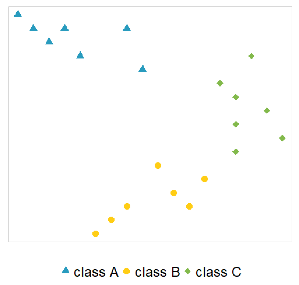
Figure 2.
One vs. all model architecture for three states.
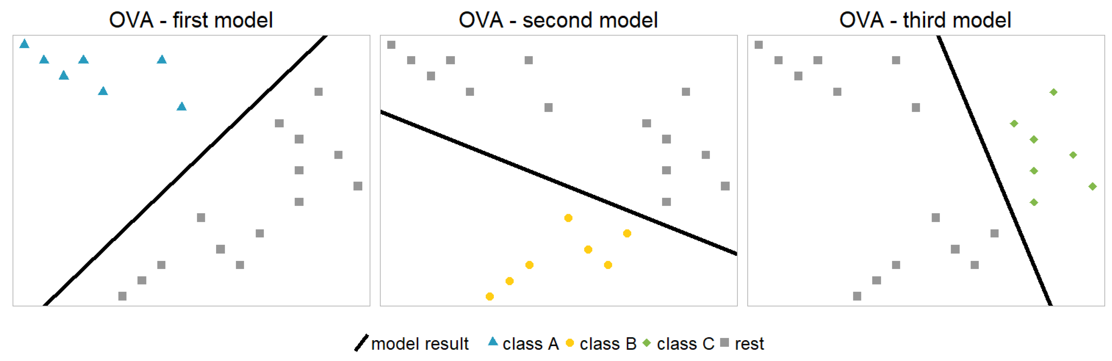
Figure 3.
One vs. one model architecture for three states.
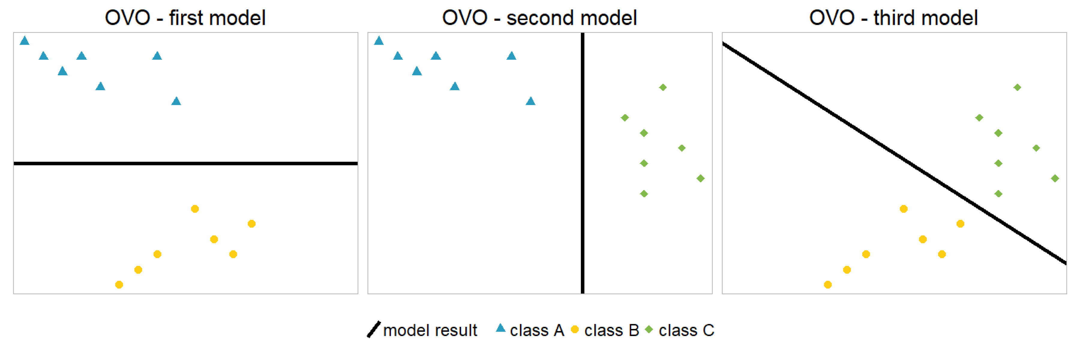
Figure 4.
Nested A model architecture for three states
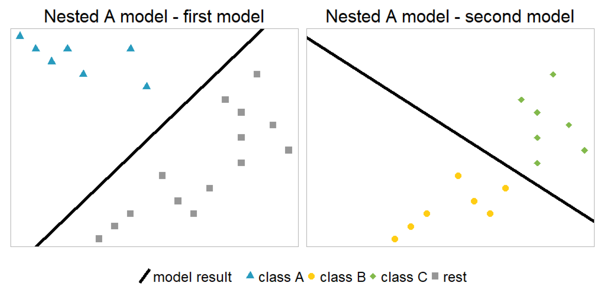
Figure 5.
MLR architecture for three states.
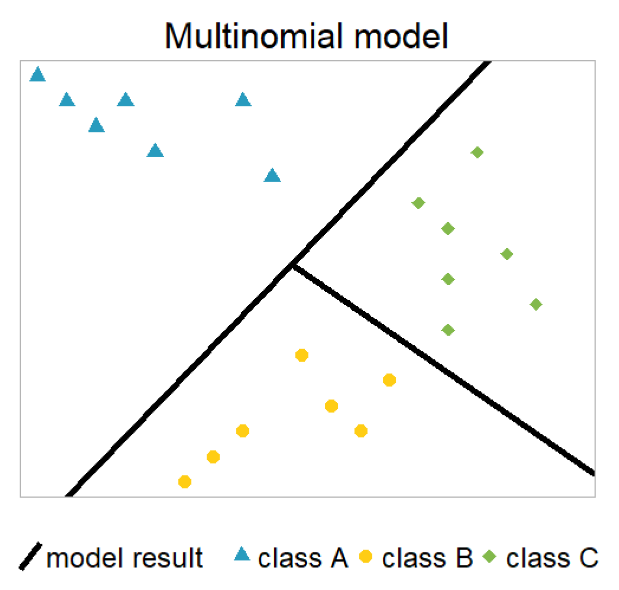
Figure 6.
Ratio of active, paid-up and lapsed contracts for different values of contract duration, including exposure.
Figure 6.
Ratio of active, paid-up and lapsed contracts for different values of contract duration, including exposure.
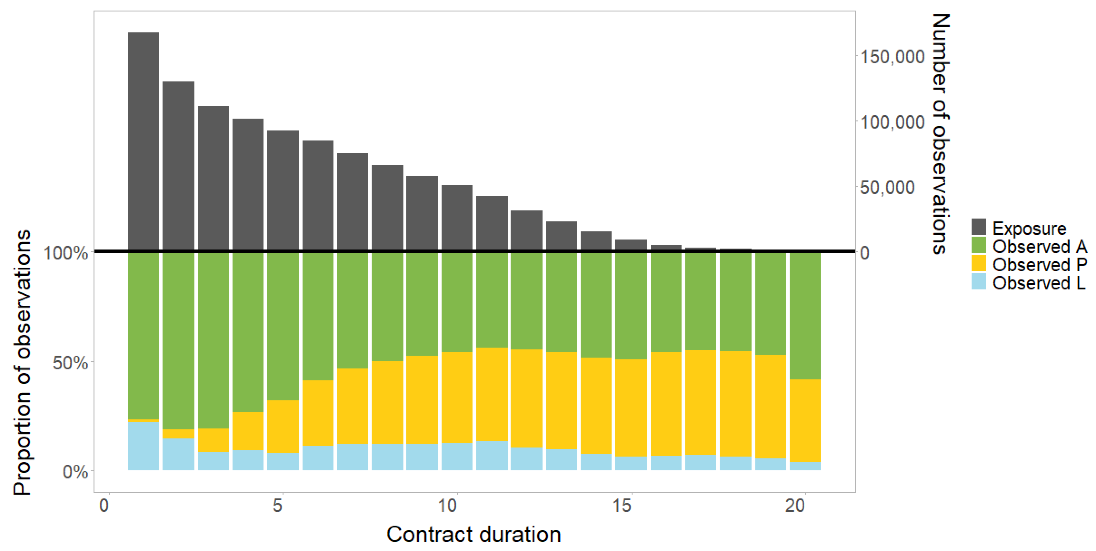
Figure 7.
Comparison of the different modelling types (colours) and transition histories (shapes) in terms of the number of parameters (x-axis) and the reduction of deviance (y-axis).
Figure 7.
Comparison of the different modelling types (colours) and transition histories (shapes) in terms of the number of parameters (x-axis) and the reduction of deviance (y-axis).
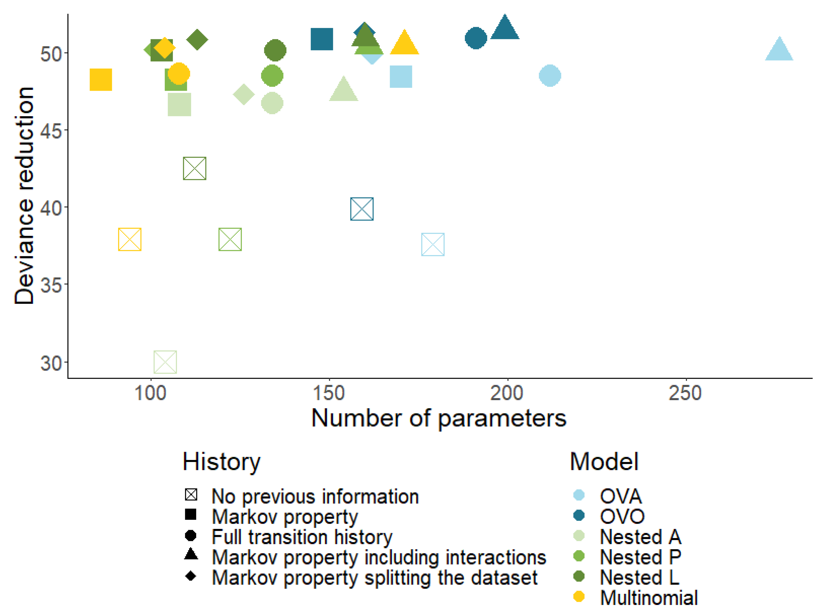
Figure 8.
Comparison of predicted lapse and paid-up rates by contract duration for different models.
Figure 8.
Comparison of predicted lapse and paid-up rates by contract duration for different models.
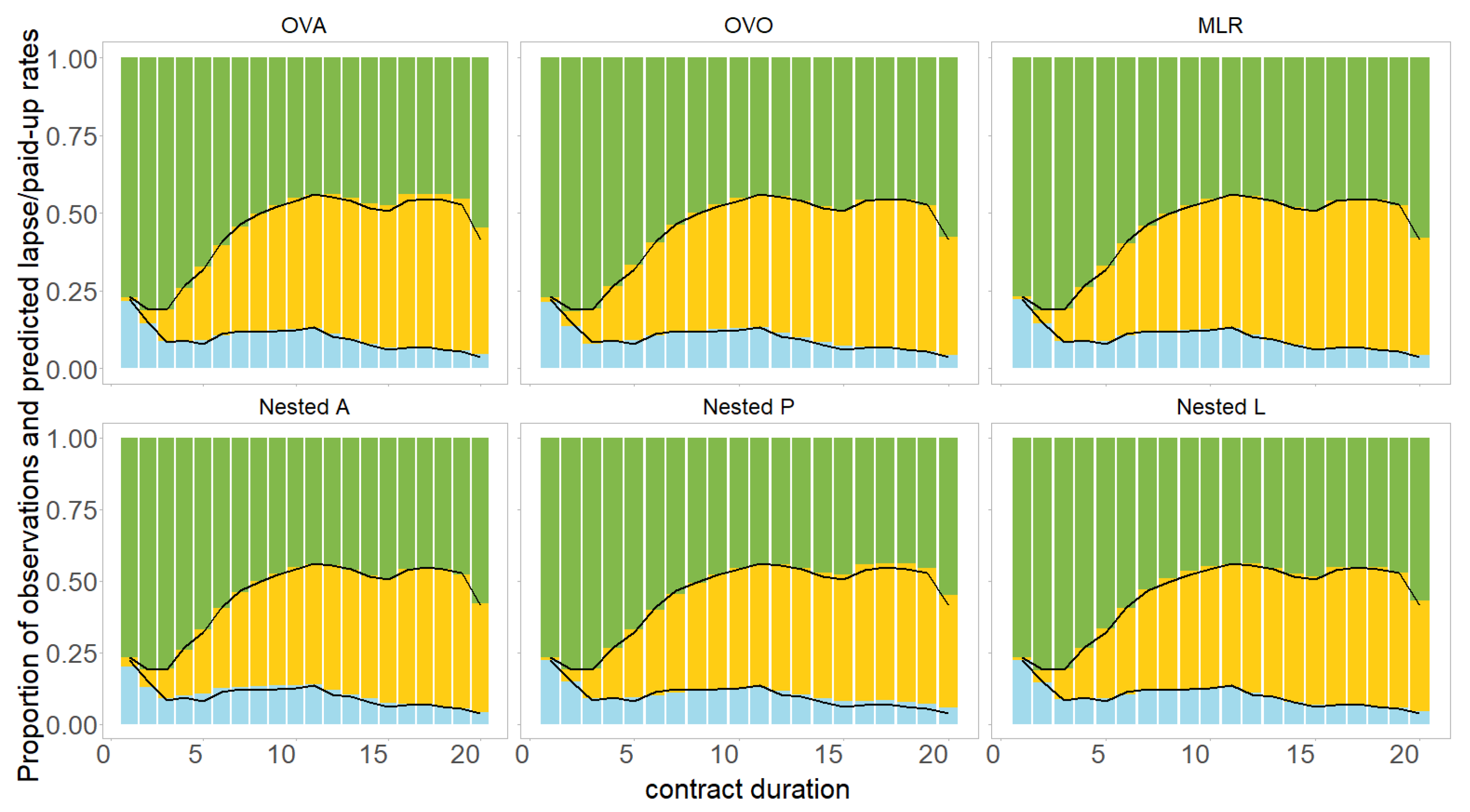
Figure 9.
Comparison of marginal effect of different models (colours) for different values of contract duration (x-axis).
Figure 9.
Comparison of marginal effect of different models (colours) for different values of contract duration (x-axis).
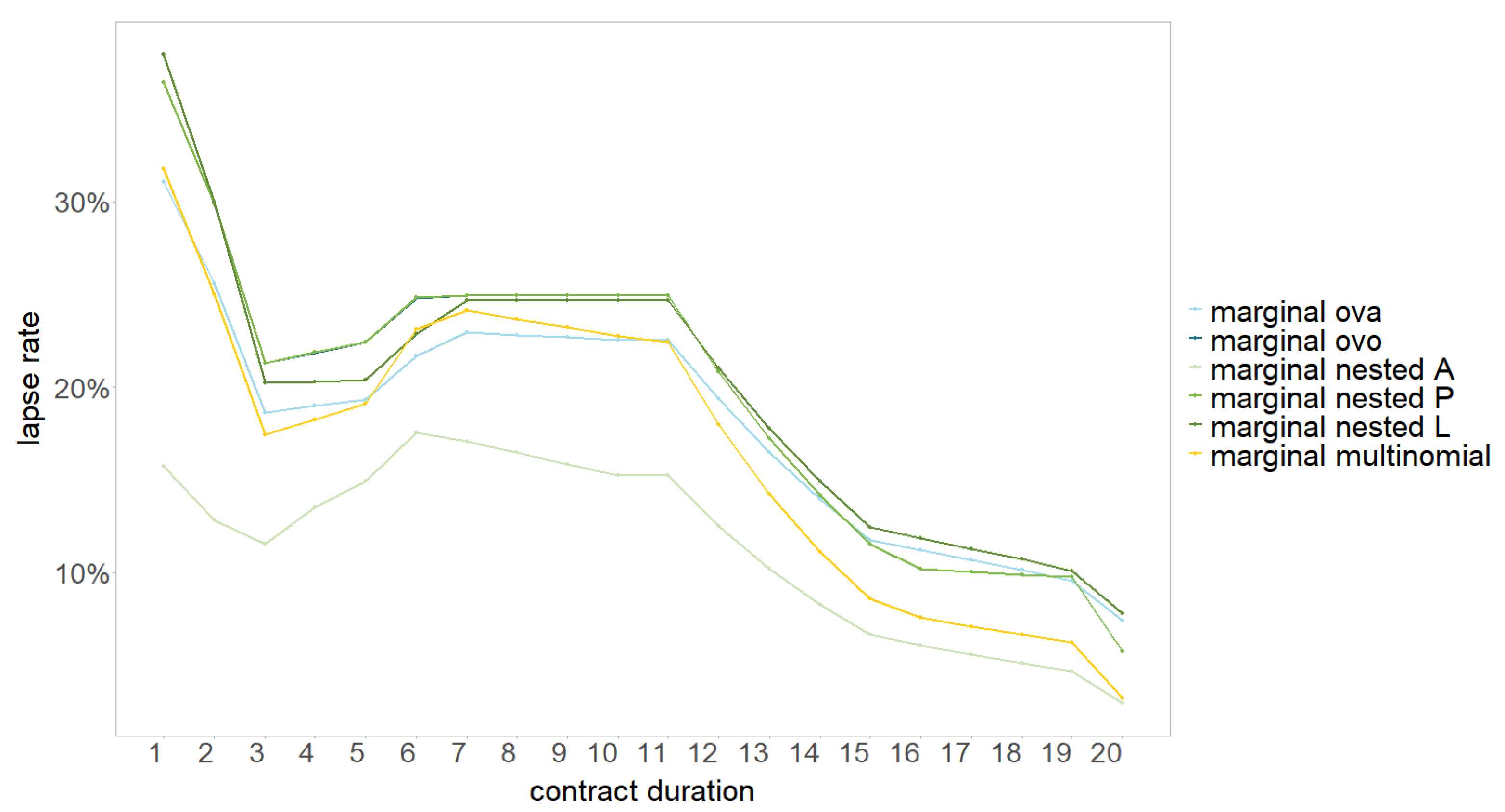
Table 1.
Penalisation terms for different model setups.
| Markov property | |||||
|---|---|---|---|---|---|
| Model |
no previous information |
Markov property |
full transition history |
including interactions |
splitting the data set |
| OVA | 1.92, 2.39, 1.63 | 1.45, 2.82, 1.48 | 1.21, 1.65, 1.48 | 1.45, 1.22, 1.12 | 2.41, 4.72, 2.96, 31.44 |
| OVO | 2.66, 1.49, 8.82 | 2.02, 1.49, 6.38 | 1.26, 1.53, 4.60 | 2.02, 1.49, 2.52 | 2.48, 3.81, 3.32, 31.44 |
| Nested A | 1.92, 8.82 | 1.45, 6.38 | 1.21, 4.60 | 1.45, 2.52 | 2.41, 3.32, 31.44 |
| Nested P | 2.39, 1.49 | 2.82, 1.49 | 1.65, 1.53 | 1.22, 1.49 | 4.72, 3.81, 31.44 |
| Nested L | 1.63, 2.66 | 1.48, 2.02 | 1.48, 1.26 | 1.12, 2.02 | 2.96, 2.48, 31.44 |
| MLR | 1.37 | 1.03 | 0.95 | 0.94 | 1.70, 31.44 |
Table 2.
Penalty types for the different covariates used for all models.
| Covariate | penalty type |
|---|---|
| contract duration | trend filtering |
| insurance type | regular |
| country | regular |
| gender | regular |
| payment frequency | fused |
| payment method | regular |
| nationality | regular |
| dynamic premium increase percentage | trend filtering |
| entry age | fused |
| original term of the contract | trend filtering |
| premium payment duration | trend filtering |
| sum insured | trend filtering |
| yearly premium | trend filtering |
| previous status | regular |
| time since paid-up | regular |
Disclaimer/Publisher’s Note: The statements, opinions and data contained in all publications are solely those of the individual author(s) and contributor(s) and not of MDPI and/or the editor(s). MDPI and/or the editor(s) disclaim responsibility for any injury to people or property resulting from any ideas, methods, instructions or products referred to in the content. |
© 2024 by the authors. Licensee MDPI, Basel, Switzerland. This article is an open access article distributed under the terms and conditions of the Creative Commons Attribution (CC BY) license (http://creativecommons.org/licenses/by/4.0/).
Copyright: This open access article is published under a Creative Commons CC BY 4.0 license, which permit the free download, distribution, and reuse, provided that the author and preprint are cited in any reuse.


