Ultra-Slow Self-Similar Coarsening of Physical Fibrillar Gels Formed by Semiflexible Polymers

1. Introduction

Semiflexible macromolecules are ubiquitous in nature.[1] A prominent example is cellulose, a semiflexible glucose polymer. As the main constituent of plant fiber, it is the most abundant organic compound on earth. DNA and proteins are other examples of important semiflexible biopolymers. Under typical conditions, many of these monofilaments form bundles[2] or fibrillar structures that assemble into transient networks with physical, i.e. reversible crosslinks.[3,4,5] These networks show remarkable properties such as strain stiffening and negative normal stresses,[6] which are rather different from networks of permanently crosslinked flexible chains that have been intensively studied using traditional network theories and simulation. For example, structure-property relationships were investigated for cellulose hydrogels, with mechanical properties found to depend on fibril length instead of concentration as expected from traditional network theories.[7] The network structure formed by physically crosslinked semiflexible polymers has an important influence on their mechanical properties.[8,9,10]

For a better understanding of these structures, it is helpful to note that they are prepared experimentally e.g. using a change of temperature, ionic strength, or pH. [1,11] Theoretically, the resulting gelation via bundling and network formation from suspensions of semiflexible polymers is interpreted as emerging from spinodal decomposition and kinetic arrest.[3,12,13,14,15] The associated reorganizations of the network can be extremely slow, in some cases exceeding several days. [16] The corresponding phenomena of slow coarsening dynamics with very long correlation lengths are known as “anomalous aging” since the time evolution and relaxation dynamics differs markedly from the more intensively studied glassy systems.[17] Nonergodicity and anomalous aging has been observed in a broad range of different systems such as amyloid fibrils,[1,18] methylcellulose,[16] alginate gels[19] and colloidal gels.[17] Considerable work is ongoing to extend traditional theoretical approaches to capture such biological soft matter systems.[9,20]

Here, we focus on reversible networks of semiflexible chains without permanent crosslinks for which classical theories can not readily be applied.[5] Although such transient structures are theoretically fascinating and highly relevant e.g. for food systems or protein-based filaments, they remain underexplored.[9] Several fundamental questions on the structure and dynamics of these networks stay unclear.[8] For cellulose derivatives often used in food systems, for example, fibrillar structures with a characteristic mean diameter of about 5 to 30 nm are observed experimentally.[11,21,22] From cryo-TEM imaging and small-angle neutron scattering (SANS), the fibril mean diameter was found to be rather independent of molecular weight, temperature and concentration, but increasing with increasing bending stiffness. [11,21] From detailed molecular simulation, these fibrils were either explained as stacked ring structures[23] or length-wise aggregation of chain molecules.[24] Different X-ray scattering experiments and cryo-TEM images seem to be more consistent with the latter scenario, suggesting axially oriented semi-crystalline chains forming the core of the fibril, interspersed with less dense regions.[25,26] Small angle X-ray scattering experiments (SAXS) experiments were used to study fibrils formed from short peptides. The change in the characteristic slope in the scattering functions was consistent with a model of thick cylinders. [27] While scattering experiments on dilute solutions of semiflexible chains are well understood,[28,29] corresponding results for networks of semiflexible chains provide valuable structural information that, however, is sometimes difficult to interpret. One difficulty is that experimentally prepared networks are often found to be spatially inhomogeneous. Mesh sizes estimated from permanent networks of rodlike particles give the right order of magnitude measured for the more compact regions, whereas much larger values are found for the more open regions.[30]

Networks of semiflexible chains show intriguing dynamics that is challenging to study not least because of their non-ergodic nature.[1,9] For example, non-diffusive compressed exponential relaxation was observed in amyloid fibrils from dynamic light scattering experiments.[31] These findings hint at structural heterogeneities of the network, but the origin of the relaxation remains unclear. Additionally, uncertainties persist regarding the different dynamic regimes and anomalous diffusion in transient networks of semiflexible chains[32], their underlying microscopic origins, and their connection to resulting mechanical properties.[9]

In general, computer simulations can help to address these questions as they offer detailed insight into structural as well as dynamical properties. They allow to detect microscopic mechanisms accompanying the coarsening process. The majority of simulations in this field seem to employ detailed atomistic or moderately coarse-grained models to investigate specific systems.[23,24,27,33,34] Because of the computational complexity of these systems only few computational studies appeared to date on the self-assembly process of semiflexible filaments and the dynamics of their networks.[34] To overcome these limitations, several coarse-grained models have been proposed that differ considerably in the level of detail retained.[33] Recently, promising multi-scale simulations have appeared that address the mechanisms of self-assembly in methylcellulose.[24] Rather than targeting such a specific chemistry, we aim at exploring universal properties of transient networks of semiflexible chains. As has been noted,[5,15] (i) the bundling of semiflexible chains into fibrils, (ii) the characteristic and rather uniform fibril diameters, and (iii) network topologies appear to be rather similar for different types of polymers. Effective attractions arise in many biopolymeric systems as a result of depletion forces.

With this in mind, we here employ a generic model of semiflexible polymers in terms of multibead-spring chains with bending stiffness and short-range attraction, building on the so-called Kremer-Grest[35] and FENE-CB[36,37,38] models. Models with qualitative similarities have been used in the past to study microphase separation in fibrillar gels,[39] the phase behavior of semiflexible attractive chains, showing a liquid-vapor coexistence region for low enough temperatures or strong enough cohesive energies,[40] and the formation of fibrous bundles,[41,42] which then assemble to form a temporary network.[15] For a two-dimensional version of the model, network structures were investigated in detail, distinguishing percolated from disintegrated networks.[43] Other recent studies used a similar model to investigate the network structure and their tensile properties, finding that high strength networks have high densities and that the cohesive energy is the most important parameter for their mechanical response.[44,45] While bead-spring models are an extremely versatile model for various polymeric systems,[46] we note in passing that other coarse-grained models have sporadically been used to study aspects of semiflexible polymer networks, such as an extended fluid particle model for the evolution and stability of networks,[47] and a discrete element method for the study of gelation, bundles, and pore size distributions.[48]

Studying the aging model system requires special care not only due to the loss of ergodicity[1] which introduces a dependence on the preparation conditions, but also due to the additional effect of the waiting time since system preparation.[49] Several simulation studies on semiflexible polymer networks artificially arrested aging by introducing sticky beads or permanent crosslinks or quenching the temperature to zero.[44,45,48] Here, we avoid such drastic interventions and study the structure, dynamics, and aging of a self-assembling, physically crosslinked semiflexible polymer system. We pay special attention to carefully prepare the systems to follow the aging process as far as possible.[12,50] To address the lack of ergodicity, we typically investigate 10 statistically independent samples, and we investigate the influence of waiting time ($t_{\mathrm{w}}$) and bending stiffness ($\kappa$) on static and dynamic properties.

2. Results and Discussion

We study in detail structural characteristics as well as dynamic properties using a multibead anharmonic (FENE) spring model of semiflexible polymers with bending stiffness $\kappa$, while all beads experience cohesive van der Waals interactions mediated through a truncated Lennard-Jones potential. Its cutoff radius determines a cohesive energy $E_{\mathrm{coh}}$ via Eq. (5). We choose initial conditions for our molecular dynamics simulations carefully to not only avoid chain overlaps but to also satisfy worm-like chain statistics of individual chains. Detailed information on the model system and simulation details as well as information on system preparation are available in Sec. 4.1. Lennard-Jones units are used throughout.

Figure 1 serves to demonstrate the richness of structures that our simple model is able to capture at a single temperature, using chains of identical length. It shows projections of snapshots of various systems at a bead number density of $\rho =0.05$. This density we determined from a series of NPT simulations for pressure $P=0$ for intermediate values of bending stiffness $\kappa$. For better comparison we then fixed $\rho =0.05$ in NVT simulations for all systems and $\kappa$ values investigated. The systems shown in Figure 1 were simulated for a relatively short time, up to time $t_{\mathrm{w}}={10}^4$ since system preparation. Varying the cohesive energy $E_{\mathrm{coh}}$ (horizontally) and bending stiffness $\kappa$ (vertically) is found to lead to different structures. For small $E_{\mathrm{coh}}\lesssim T$, isolated chains are found that become more straight with increasing bending stiffness. Increasing $E_{\mathrm{coh}}$ leads to cluster and structure formation. For low $\kappa$, these clusters tend to be more compact, while larger $\kappa$ together with cohesive attractions leads to open, network-like structures.

To study these structures and resulting properties, from now on we fix a representative value of the cohesive energy ($E_{\mathrm{coh}}=1.4$) and focus on the influence of $\kappa$ on static and dynamic properties. With this value of $E_{\mathrm{coh}}$ we make sure to include compact as well as open structures in our study (green framed regime in Figure 1).

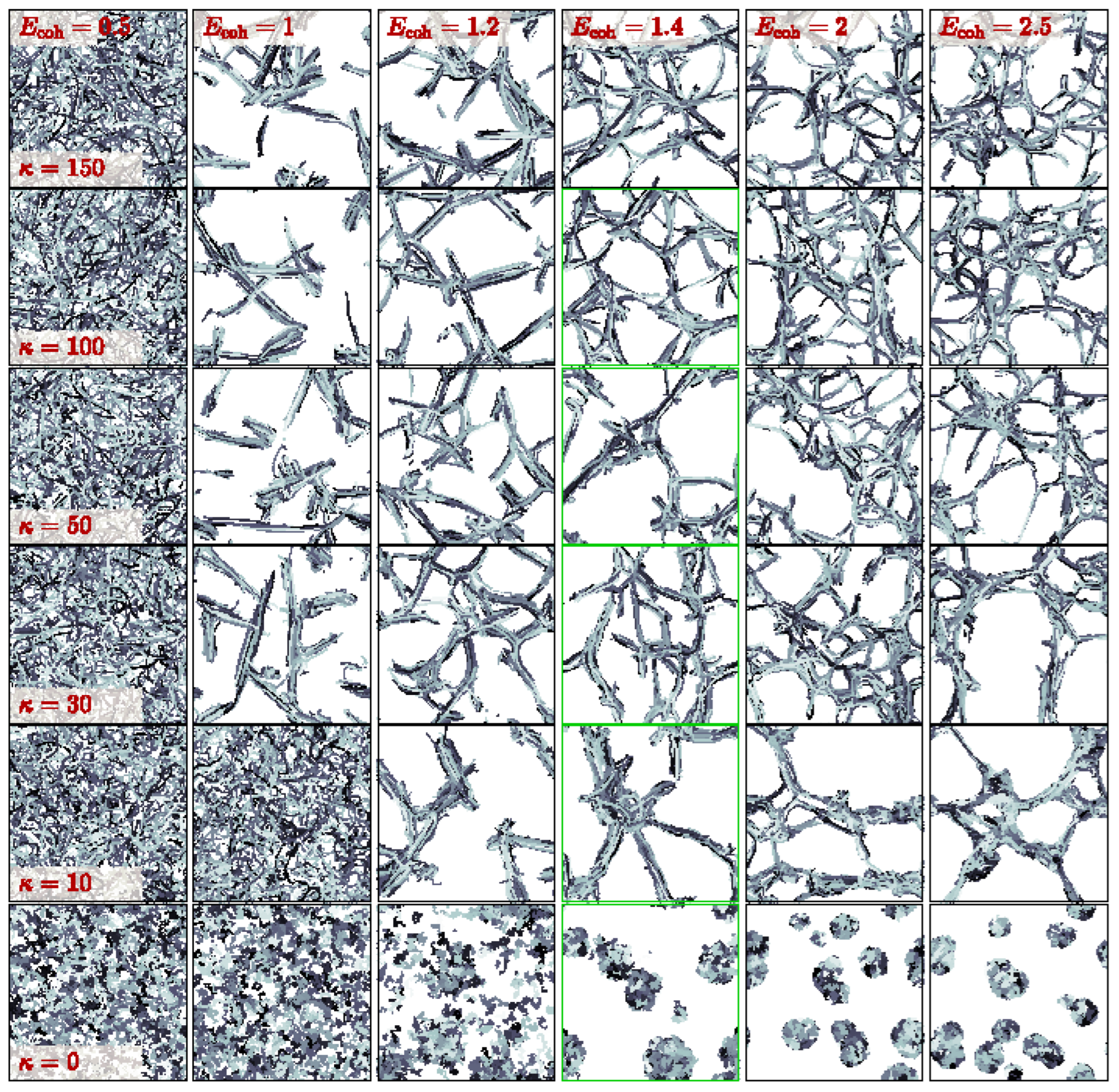
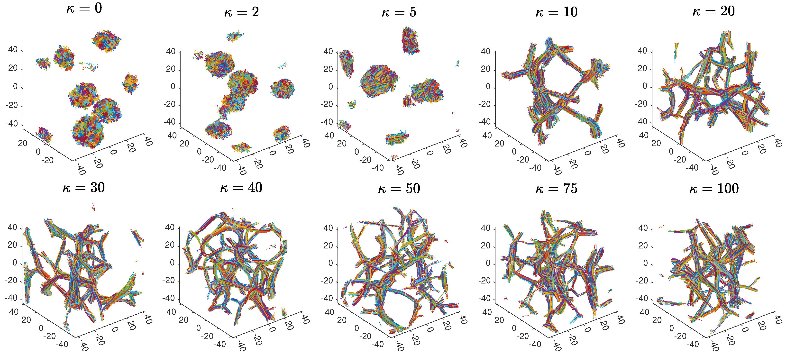
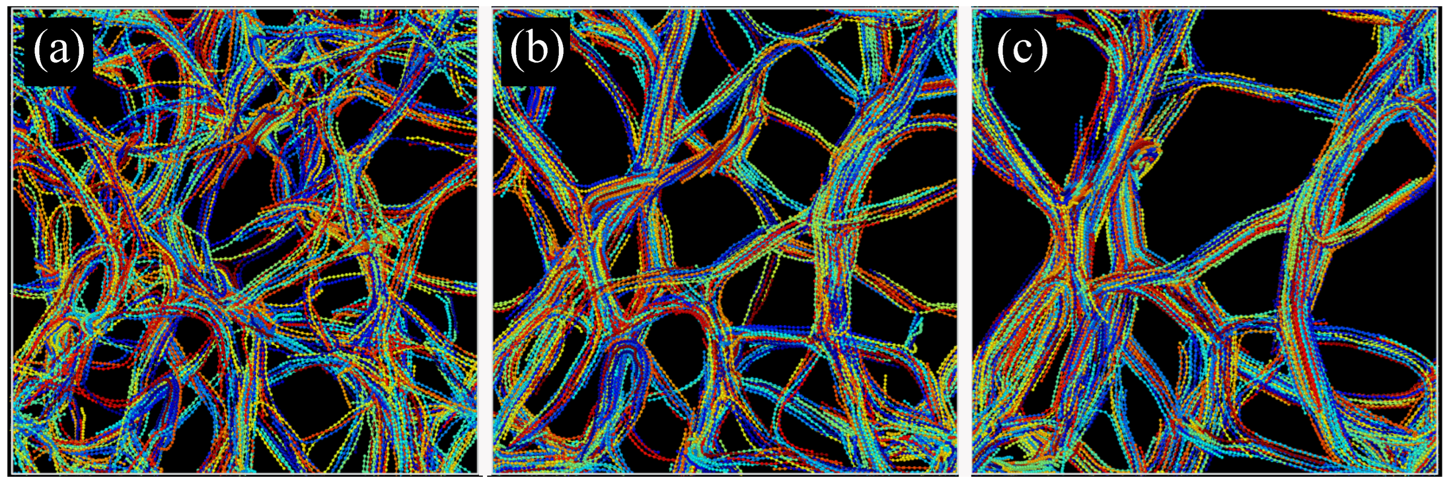
2.1. Initial Observations

Snapshots of representative system configurations with $N_c=1000$ chains, polymerization degree $N=30$, thus $N_b=N_{c}N=30000$ beads in total are shown at a late stage of a typical run in Figure 2. Different panels in the figure correspond to different values of bending stiffness $\kappa$. These figures are thus not only close-up three-dimensional versions of the corresponding panels of Figure 1, but show those systems after considerable longer times $t_{\mathrm{w}}$. For rather flexible chains, $\kappa \lesssim 5$, droplets are formed by several coiled chains. For more rigid chains, $\kappa \gtrsim 5$, strongly bent configurations are energetically too unfavorable: droplets mixed with short, near-cylindrical bundles ($\kappa =5$) as well as system-spanning networks of long, fibrillar bundles ($\kappa \gtrsim 10$) are formed. Thus, the snapshots suggest both an ordering and a percolation transition as the bending stiffness increases. For a few (2 out of 10 in each case) samples within the transition regime we also observed thick filaments percolated in one dimension for $\kappa =5$, and networks for $\kappa =10$ percolated in two dimensions (supplementary Figure S14). We will come back to these points later.

As a first proxy for structure evolution, we monitor the mean pair energy ($e_{\mathrm{pair}}$) and mean bending energy per particle ($e_a$) as a function of $t_{\mathrm{w}}$. The pair energy $e_{\mathrm{pair}}$ is defined as the mean Lennard-Jones energy (4) per bead. As can be seen from Figure 3, $e_{\mathrm{pair}}$ and $e_a$ both decrease with time as expected for equilibration. As a decreasing $e_a$ reflects local bending stiffening, chains tend to straighten out in the course of $t_{\mathrm{w}}$. The decrease of $e_{\mathrm{pair}}$ suggests an increase in local ordering and decrease in surface area. When plotting these two quantities on a linear time scale, Figure 3(a) and (b), one might be inclined to conclude that equilibration is mainly achieved. However, closer inspection and using a logarithmic time scale (Figure 3(c) and supplementary Figure S7) reveals a very slow ongoing relaxation with a relaxation time that increases significantly with system age.

Recall that aging and ultra-slow coarsening have been observed in several network-forming soft matter systems.[12,13,14,16,17,18,19,47,49,50,51,52] The essential absence of complete relaxation in these systems has been attributed to phase separation and quasi-arrested spinodal decomposition, explaining the similar phenomenology observed in rather different systems.[12,52,53] In particular, spinodal decomposition has been identified as the driving force for bundling and network formation in polymeric systems similar to the one studied here.[3,14,15] In the following, we study and discuss the aging and coarsening behavior. As an interesting first observation, Figure 3(d) shows a linear relation between the pair and bending energy during relaxation, indicating that coarsening proceeds along certain rules.

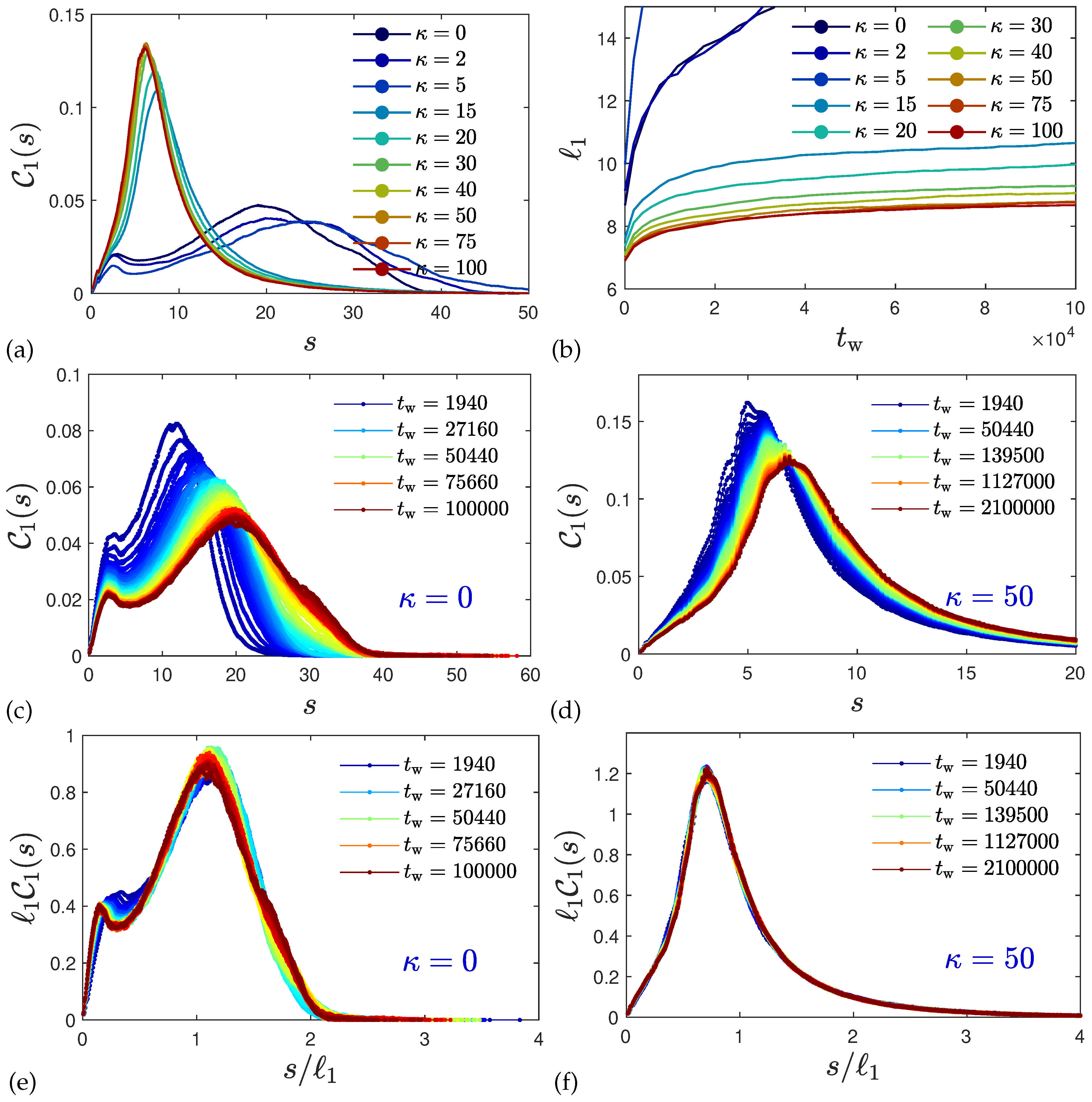
2.2. Structure Analysis and Static Properties

We begin by analyzing the structures that are formed for different $\kappa$ and the corresponding static properties. In view of the ultra-slow ongoing relaxation, we perform all structural analysis at different $t_w$.

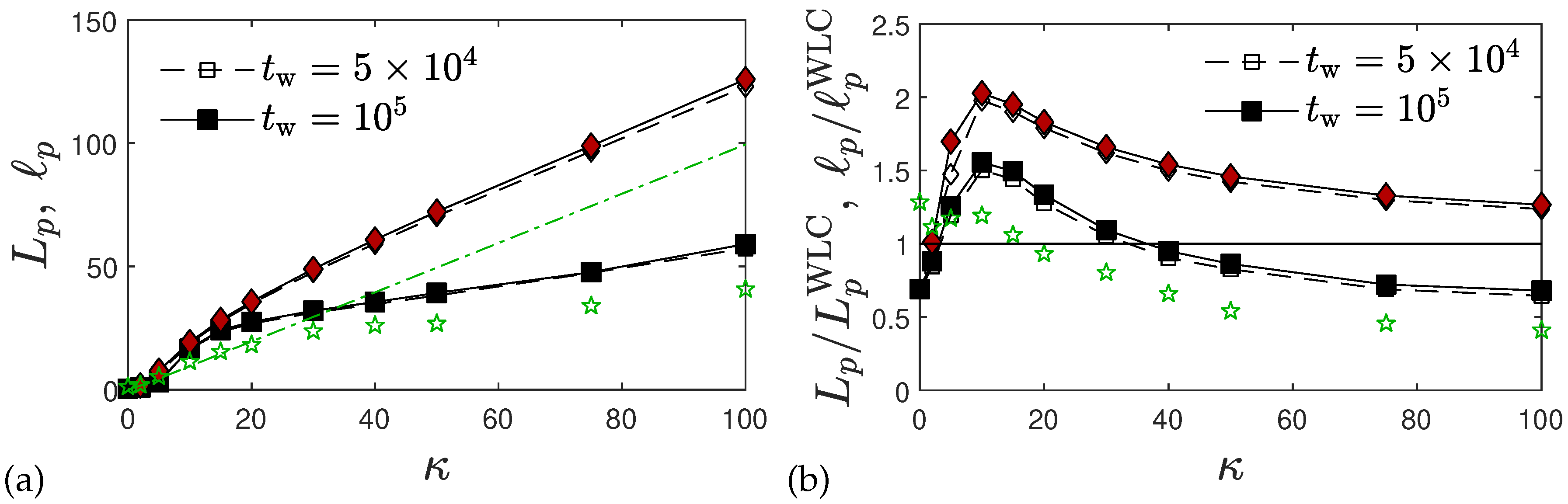
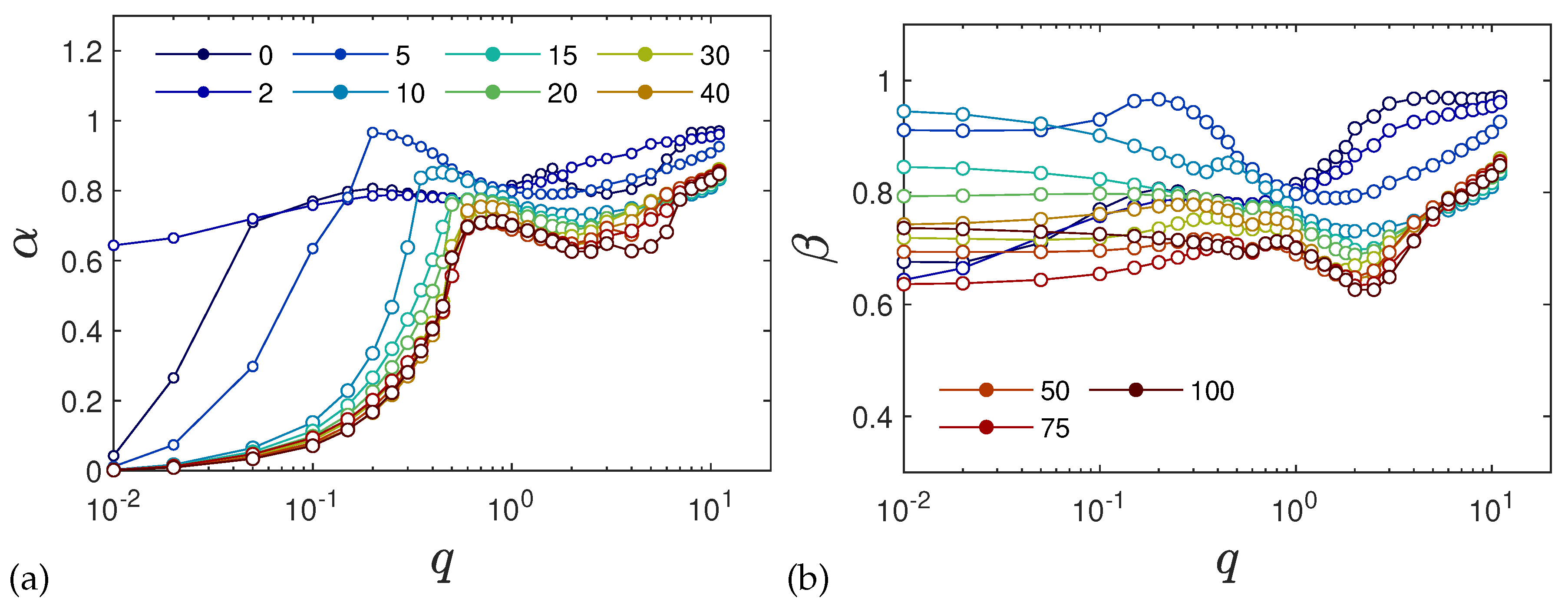
2.2.1. Single Chain Structure Factors and Persistence Lengths

The static structure factor (Sec. 4.2) is a fundamental quantity routinely determined in both scattering experiments and simulations, as it encapsulates key structural information. Experimentally, it offers a unique method for probing features across different length scales, particularly in systems that are too small to be studied directly through microscopy techniques.

We first present results for the isotropic single-chain structure factor, $S_{\mathrm{sc}}\left(q\right)$, defined in Eq. (8), as function of wave number q. Experimentally, $S_{\mathrm{sc}}$ can be measured through small-angle neutron scattering (SANS) on samples where a small fraction of polymer chains have been selectively labeled. Figure 4(a) shows $S_{\mathrm{sc}}$ obtained for various values of the bending stiffness $\kappa$. Data averaged over two different ranges of waiting times $t_{\mathrm{w}}$ are quasi indistinguishable. As $\kappa$ increases we see a transition from a near-random walk behavior ($S_{\mathrm{sc}}\sim q^{-2}$) to an extended range of q values where $S_{\mathrm{sc}}\sim q^{-1}$ shows the typical scaling of rod-like objects. It is remarkable that despite chain-chain interactions, $S_{\mathrm{sc}}$ can still be described very well by the scattering function of the discrete wormlike chain (WLC) model (for details see Sec. 4.2). However, the required values of persistence lengths differ from the local persistence lengths ${\ell }_p$ that are inferred from the bending energy $e_a$ (Sec. 4.3).

To confirm this observation, we analysed directly two single-chain properties: the mean-square end-to-end distance $\langle R^2\rangle$ and the gyration radius $R_g$. For the WLC model, these quantities are given in terms of the number of beads per chain N and the global persistence length $L_p$ (see Sec. 4.3 and supplementary Figure S10). Values for $L_p$ extracted from the ratio $\langle R^2\rangle /R_g^2$ are shown in Figure 5 (time series in supplementary Figure S7) together with those extracted from the fits of the single chain structure factor. The latter are systematically smaller but follow the same trend: the effective global persistence length initially increases approximately linearly with $\kappa$, before crossing over to a much slower increase for $\kappa \gtrsim 20$. The local effective persistence length ${\ell }_p$ evaluated from the bending energy agree with those from $R_g$ for $\kappa \lesssim 2$, but clear differences are seen for stiffer chains where bending energies imply larger values of ${\ell }_p$ compared to $L_p$’s from the gyration radius. For our systems, we suspect that the scale-dependency of the persistence length of chains within the fibrous networks may be caused by the formation of junctions connected by strands whose lengths do not exceed $L_p$ by far.

Figure 4. Structure factors. (a) $S_{\mathrm{sc}}\left(q\right)$ and (b) $S\left(q\right)$ averaged over $t_{\mathrm{w}}\in [0,{10}^5]$ (dashed) and $t_{\mathrm{w}}\in [5\times {10}^4,{10}^5]$ (solid). In panel (a) power laws $q^{-1}$ (rod-like) and $q^{-2}$ (gaussian) have been added to guide the eye. (b) The Porod $q^{-4}$-regimes, signaling well defined interfaces in both the unpercolated ($\kappa <10$, spherical and cylindrical clusters) and percolated regimes ($\kappa \ge 10$, filamentous networks) are highlighted.

Figure 4. Structure factors. (a) $S_{\mathrm{sc}}\left(q\right)$ and (b) $S\left(q\right)$ averaged over $t_{\mathrm{w}}\in [0,{10}^5]$ (dashed) and $t_{\mathrm{w}}\in [5\times {10}^4,{10}^5]$ (solid). In panel (a) power laws $q^{-1}$ (rod-like) and $q^{-2}$ (gaussian) have been added to guide the eye. (b) The Porod $q^{-4}$-regimes, signaling well defined interfaces in both the unpercolated ($\kappa <10$, spherical and cylindrical clusters) and percolated regimes ($\kappa \ge 10$, filamentous networks) are highlighted.

Figure 5. Persistence lengths versus $\kappa$ at two different waiting times $t_{\mathrm{w}}$. (a) Global $L_p$ extracted from the ratio $\langle R^2\rangle /R_g^2$ (black squares), using the discrete WLC expression (), local ${\ell }_p$ obtained from the specific bending energy $e_a$ (red diamonds), and $L_p$ estimated upon fitting the $S_{\mathrm{sc}}$ by the WLC model (green pentagons). Dot-dashed green line $L_p^{\mathrm{WLC}}={\ell }_p^{\mathrm{WLC}}=-b/ln\left[\mathcal{L}(\kappa /k_{\mathrm{B}}T)\right]$ for the ideal WLC has been added to guide the eye. (b) Same data as shown in (a), here relative to the the ideal WLC. Global $L_p$’s obtained using the bond length b and $R_g^2$, or alternatively $\langle R^2\rangle$ alone are basically identical to those obtained from the ratio. The single chain structure factor $S_{\mathrm{sc}}\left(q\right)$ (Figure 4) is very well approximated by the WLC structure factor, using $L_p$ values that are slightly below the ones obtained from the ratio.

Figure 5. Persistence lengths versus $\kappa$ at two different waiting times $t_{\mathrm{w}}$. (a) Global $L_p$ extracted from the ratio $\langle R^2\rangle /R_g^2$ (black squares), using the discrete WLC expression (), local ${\ell }_p$ obtained from the specific bending energy $e_a$ (red diamonds), and $L_p$ estimated upon fitting the $S_{\mathrm{sc}}$ by the WLC model (green pentagons). Dot-dashed green line $L_p^{\mathrm{WLC}}={\ell }_p^{\mathrm{WLC}}=-b/ln\left[\mathcal{L}(\kappa /k_{\mathrm{B}}T)\right]$ for the ideal WLC has been added to guide the eye. (b) Same data as shown in (a), here relative to the the ideal WLC. Global $L_p$’s obtained using the bond length b and $R_g^2$, or alternatively $\langle R^2\rangle$ alone are basically identical to those obtained from the ratio. The single chain structure factor $S_{\mathrm{sc}}\left(q\right)$ (Figure 4) is very well approximated by the WLC structure factor, using $L_p$ values that are slightly below the ones obtained from the ratio.

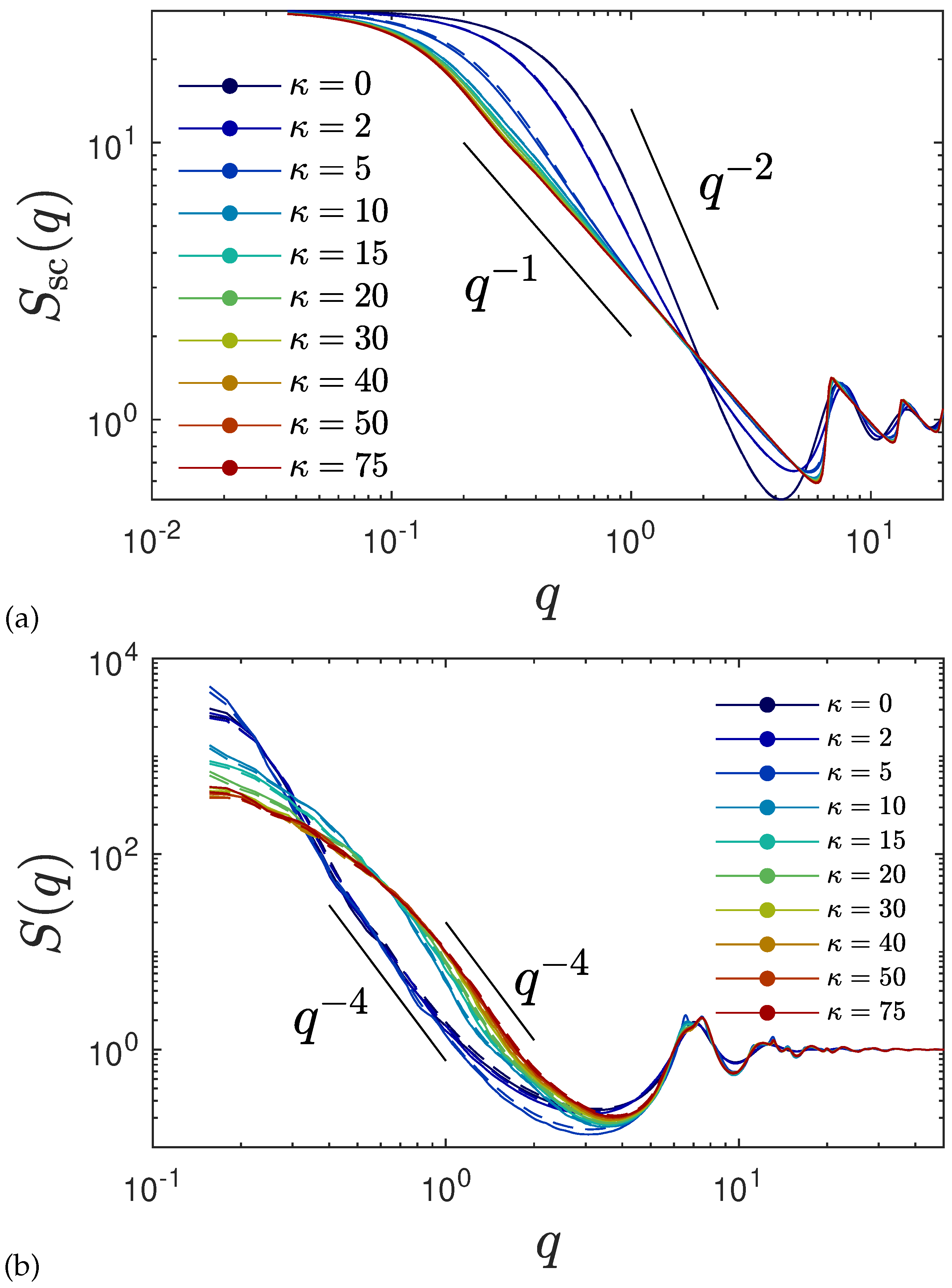
2.2.2. Structure Factor

The full static structure factor $S\left(q\right)$ as defined in Eq. (7) accounts for all beads in the system, regardless of bond topology. Figure 4(b) presents $S\left(q\right)$ for the same range of bending stiffness $\kappa$ as in Figure 4(a). At first glance, two different families of curves can be distinguished in Figure 4(b): (i) the one for rather flexible chains ($\kappa \le 5$) forming droplet phases and (ii) the one for stiffer chains $\kappa \ge 10$ forming percolated fibrous networks. These findings corroborate earlier observations from the snapshots in Figure 2 which indicate a transition from a droplet- to a network-forming phase as $\kappa$ increases from $\kappa =5$ to $\kappa =10$.

At large scattering vectors ($q\ge 7$) , both systems exhibit the usual diffuse scattering peaks reminiscent of the bead-bead intra and inter-chain correlations.

For droplet systems, the $S\left(q\right)$ curves show no distinct peaks or fringes, indicating that the dense globular droplets are quite irregular in shape and/or polydisperse. However, fringes of small amplitudes are detectable in individual samples if averaged over the last 100 time units only (data not shown). Due to the limited size of our systems, the Guinier regime ($q{R}_g<1$) is not reached and no correlation peaks corresponding to a characteristic droplet-droplet distance are observed. In the probed (intermediate) q range, the scattering curves follow a Porod-like behavior $S\left(q\right)=K_{\mathrm{p}}/q^4$, and are therefore dominated by the scattering arising from the sharp density change at the droplet interfaces. For spherical droplets of radius R, this regime appears for $q>q_{\mathrm{c}}$ where $q_{\mathrm{c}}\propto 1/R$. The proportionality constant $K_p$, setting the level of $S\left(q\right)$ in the Porod regime, is given in our case by $K_{\mathrm{p}}=2\pi {\rho }_f^2{A}_f/N_b$, where ${\rho }_f$ is the bead number density in the dense polymer phase and $A_f$ its total surface area.[54]

For the percolated network structures, the shape of scattering curves is consistent with that expected for polydisperse cylindrical objects. A narrower Porod regime is observed ($q_{\mathrm{c}}\propto 1/d$ with d denoting a cylinder diameter) whose onset slightly shifts to higher q with increasing stiffness, indicating a slight decrease in fiber diameters which saturates at large $\kappa$. The levels of $S\left(q\right)$ in the Porod regime are significantly higher than those for the droplet systems, in agreement with the higher interfacial area of the fibrous network structures. In Figure 4, the structure factors averaged over two different ranges of waiting times $t_{\mathrm{w}}$ since system preparation are nearly undistinguishable. Yet a slight increase in the Porod constant over time is hinted. Overall, the structure factors data allow to clearly classify our systems into two types of structures: globular and cylindrical. However, the limited low-q range and the absence of prominent features in the curves make it challenging to extract precise quantitative structural information.

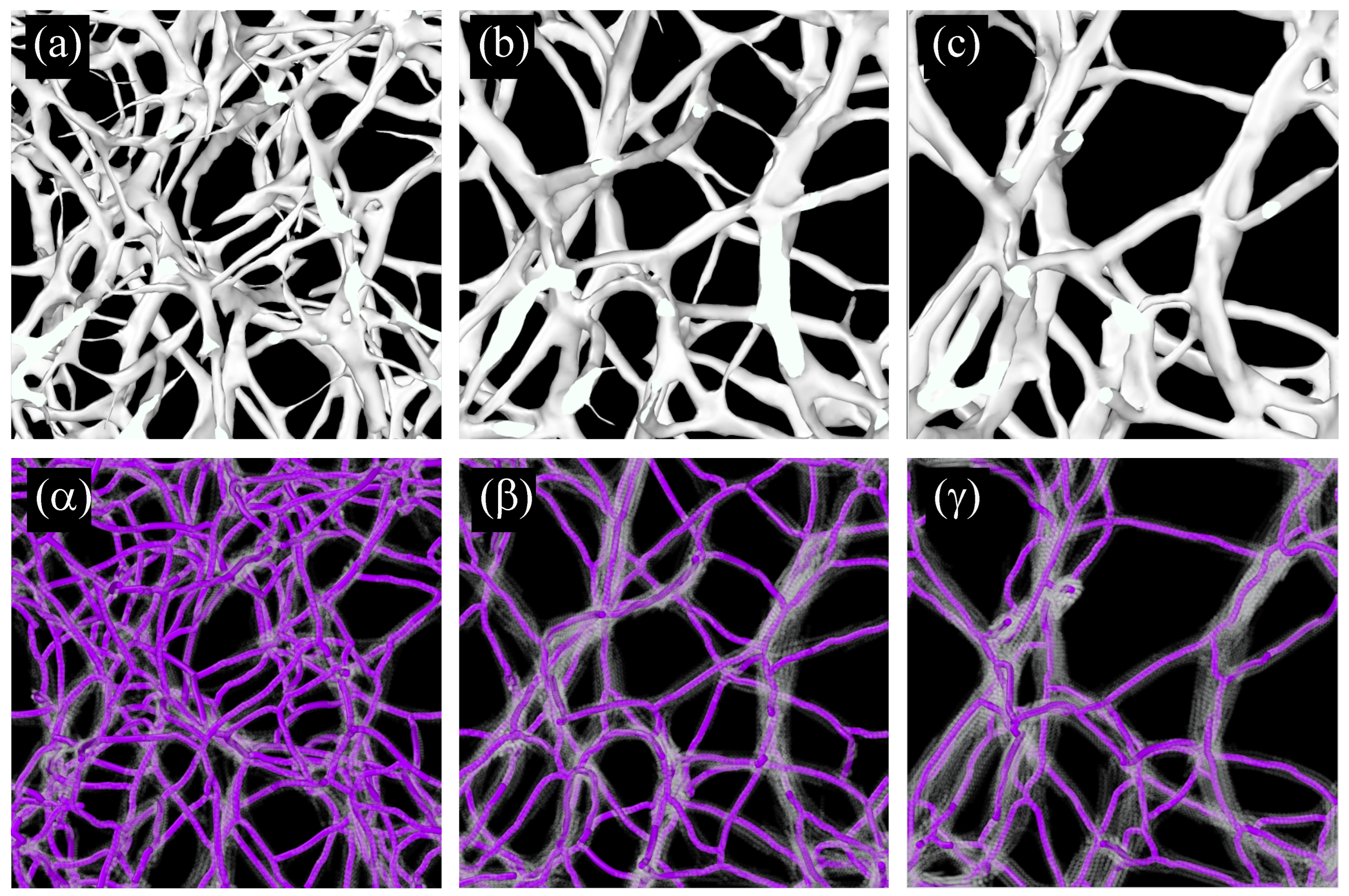
2.2.3. Real Space Structural Analysis

While the time-averaged structure factors capture essential, experimentally accessible parameters such as $R_g$, $L_p$, ${\rho }_f$, $A_f$ in reciprocal space, our simulation provides access to the full temporal evolution of not only these, but of additional structural quantities directly in real space. A qualitative picture readily emerges based on animated sequences of the chain trajectories (see supplementary Sec. S7, movies A-J). They provide a visual impression about the self-assembly of chains into bundles and the formation and evolution of the network or droplet structures. To quantitatively capture key aspects of these observations for further analysis, we extract the number of clusters, strands, junctions and loops, critical bonds, the mean strand length and bundle thickness, chord length and pore size distributions, using methods such as a skeleton-algorithm, Voronoi decomposition, Euler’s topological identities and the Cauchy-Crofton formula.

First, our cluster analysis (Sec. 4.5.1) confirms a percolation transition where a single, system-spanning infinite cluster ($C=1$) is formed for semiflexible chains with $\kappa \ge 10$ (Figure 21). For more flexible chains with $\kappa \le 5$, several droplets of isolated smaller clusters of coiled chains are seen. Those clusters tend to coagulate with time for $\kappa \le 2$, while short bundles of aligned chains tend to be more stable for $\kappa =5$. Note that the precise location of the percolation transition also depends on the value of the cohesive energy $E_{\mathrm{coh}}$ and moves to larger $\kappa$ as $E_{\mathrm{coh}}$ decreases. While there are no critical (load-bearing) bonds[55] (Sec. 4.5.1) for the droplet systems, the number of critical bonds in the percolated networks ($\kappa \ge 10$) is quite insensitive to $\kappa$. The system at $\kappa =30$ attains the largest number (roughly 600) of critical bonds and may thus be envisioned as the most mechanically stable system under study (this prediction could be scrutinized e.g. by mechanical tests).

Figure 6(a–f) show the ensemble-averaged strand length $L_f$ and thickness $d_f$ (Sec. 4.5.4), number of edges E, junctions J, and loops $L_{\circ }$ (Sec. 4.5.3), and the mean pore size $r_{\mathrm{pore}}$ introduced by Gelb and Gubbins [56] (Sec. 4.5.5), respectively, as a function of the bending stiffness $\kappa \ge 10$ for percolated systems at two selected values of the waiting time, $t_{\mathrm{w}}=5\times {10}^4$ and $t_{\mathrm{w}}={10}^5$. All but the pore size have been obtained with the help of skeletons (Sec. 4.5.2, supplementary Figure S3), whose flexible multibead strands (of mean contour length $L_f$) follow the centerlines of the filamentous bundles, until they terminate at one- (dangling ends) or higher-functional junctions. Each skeleton bead is easily characterized by its functionality, and from the knowledge of the number $n_f$ of skeleton beads with given functionality f, and the number C of clusters, one has direct access to the number of edges, junctions, vertices, and loops without inspecting the network further. We observe that $L_f$, strand diameter $d_f$ (≃ mean thickness of the polymeric strands centered at the skeleton) and pore radius $r_{\mathrm{pore}}$ decrease monotonically with increasing bending stiffness (at given $t_{\mathrm{w}}$) until reaching a plateau for large $\kappa$. The number of edges, junctions, and loops exhibit the opposite trend. The stiff systems therefore exhibit more junctions, thinner filaments, and a smaller pore radius compared with the flexible systems at comparable age, but upon aging the stiffer systems much further, their topological characteristics tend to become similar to those of the more flexible, younger systems.

For an ideal network free of dangling ends and solely composed of three-functional junctions the number of junctions equals the number of vertices, the number of edges is 3/2 times the number of junctions, $E/J=3/2$, and the number of loops is $L_{\circ }=C+E/3$. As mentioned, our coarsed percolated networks all exhibit a single infinite cluster, $C=1$. From the quantities displayed in Figure 6(c,d,f) one can infer the number of dangling ends, $n_1=C+E-J-L_{\circ }$, which is relatively small, and a mean functionality of junctions, ${\overline{f}}_J=(2E-n_1)/J$, close to three. To be specific, we find at $t_{\mathrm{w}}={10}^5$ that the ratio of dangling ends to three-fold junctions, $n_1/n_3$, monotonically decreases from about 0.07 at $\kappa =10$ to 0.04 at $\kappa =100$, while the ratio of four-fold to three-fold junctions, $n_4/n_3$, monotonically and weakly increases with $\kappa$ from about 0.01 to 0.03 over the same $\kappa$ range and there is a negligible amount of higher-functional junctions. In more quantitative terms, for the ratio $E/J$ we obtain a nearly constant value of $\approx 1.535$ over the whole range of $\kappa$ values, while $L_{\circ }/(1+E/3)$ moderately increases from 0.93 to 0.97 between $\kappa =10$ and $\kappa =100$. For this reason, our networks are near-ideal three-functional at $t_{\mathrm{w}}={10}^5$, and they approach this stage in a manner that is captured by the time series of functionalities (supplementary Figure S4). Even though systems with different $\kappa$ age at different rates, the mentioned trends are unaffected by the choice of $t_{\mathrm{w}}$.

Our results concerning $d_f$ are in qualitative agreement with earlier simulations of a similar model system.[45] In comparison to the static structure factor shown in Figure 4, the quantities $L_f$, $d_f$, $L_{\circ }$ and also $r_{\mathrm{pore}}$ show more clear differences for the two values of $t_{\mathrm{w}}$. Mass conservation arguments can be used, as shown in Sec. 4.6.4, to heuristically derive a scaling relation between the mean filament diameter $d_f$ and the mean pore size,

$$d_f\sim r_{\mathrm{pore}}.$$

(1)

Figure 6(g) shows a parametric plot of the mean filament diameter $d_f$ versus the mean pore radius $r_{\mathrm{pore}}$. For all values $\kappa \ge 10$ and different waiting times, we find that our data follow the scaling relation (1) reasonably well. We note that a corresponding relation for a two-dimensional transient network of semiflexible chains was also found to hold rather well.[43] In addition, we observe from Figure 6(h) that the product of the number of loops and the pore volume, $L_{\circ }{r}_{\mathrm{pore}}^3$, is approximately constant. Since $L_{\circ }/J$ reflects the total amount of loops per branch point including primary and higher-order loops, its value does help to judge about the modulus or fracture energies, which are presumably better captured by the cycle rank,[57] or the above-mentioned amount of critical bonds.

The values shown in Figure 6 provide descriptions of the network structure in terms of mean quantities, and thus do not allow us to draw conclusions about possible heterogeneities. Therefore, we show in Figure 7(a) and (b) the weighted distribution of filament lengths $L_f$ and diameters $d_f$, respectively, for selected values of the bending stiffness $\kappa$. We find that not only the mean value of $L_f$ remains approximately constant for $\kappa \gtrsim 40$ (see Figure 7(a)), but the whole distribution, positively skewed, hardly changes in this regime as $\kappa$ increases. For the filament diameter $d_f$ on the other hand, the probability distribution is more gaussian and moves to lower values as $\kappa$ increases, approaching a limiting distribution only at higher values. Both distributions are relatively broad.

Within the same spirit, in Figure 8, we show the pore size distribution G-$P_{\mathrm{pore}}^{\mathrm{cum}}\left(r\right)$, i.e. the cumulative probability that the largest sphere, containing a randomly chosen point within the void space, and not overlapping with any of the beads, has a radius smaller or equal than r. For more information on this quantity see Sec. 4.5.5. For small values of $\kappa$, the system is unpercolated and the distributions have to be interpreted with care. For larger $\kappa$, the vast majority of pores have a radius between around 10 and 20. Together with the smooth increase of G-$P_{\mathrm{pore}}^{\mathrm{cum}}\left(r\right)$ we conclude that the networks formed do not show pronounced heterogeneities. We also observe that the mean pore radii $r_{\mathrm{pore}}$ very slightly get larger with increasing waiting time (supplementary Figure S7), in agreement with Figure 6(e). For comparison, Torquato’s[58] cumulative T-$P_{\mathrm{pore}}^{\mathrm{cum}}\left(r\right)$, defined in supplementary Sec. S4, is shown in supplementary Figure S9. The T-$P_{\mathrm{pore}}^{\mathrm{cum}}\left(r\right)$ is known to underestimate the pore radius,[59] but is much less time-consuming to extract with high accuracy. While the pore size distributions do not reveal any qualitative peculiarities, they will help us to demonstrate self-similarity during ultra-slow coarsening.

Another important, convenient measure of the characteristic length scales of a network is given by the so-called chord length distribution (Sec. 4.5.6).[60] Roughly speaking, the chord length s is the distance between two consecutive network-pore interfaces along a virtual line through the system.[50,52,61] Figure 9(a) shows the weighted chord length distribution ${\mathcal{C}}_1\left(s\right)$ of the dense polymeric phase for several values of the bending stiffness $\kappa$. The corresponding weighted chord length distribution of the void space ${\mathcal{C}}_0\left(s\right)$ has been extracted and analyzed as well (Figure 22). In the droplet phase for $\kappa \le 5$, ${\mathcal{C}}_1\left(s\right)$ shows a pronounced peak at small s ($s\approx 2$), a weaker and broader peak at larger s ($s\approx 10\dots 20$), followed by a relatively long tail. The broad peak around $s\approx 10\dots 20$ can be related to the typical size of droplets (Figure 2). In the network-forming phase for $\kappa >10$, the shape of the chord length distribution ${\mathcal{C}}_1\left(s\right)$ changes to a unimodal shape. The location and height of the peak are found to be rather insensitive to the precise value of $\kappa$ in this regime. We note that the most probable chord length decreases weakly with increasing $\kappa$ from about $s\approx 7$ ($\kappa =10$) to $s\approx 4.5$ ($\kappa =100$) and is, within numerical uncertainties, identical with the mean filament thickness $d_f$ (Figure 6-b). This finding perfectly supports the conclusion that our percolated systems contain mainly near-cylindrical filaments with $L_f>d_f$.[60] We note that Figure 9(a) corresponds to a particular time $t_{\mathrm{w}}={10}^5$. The time-dependence and remaining panels of Figure 9 will be discussed next.

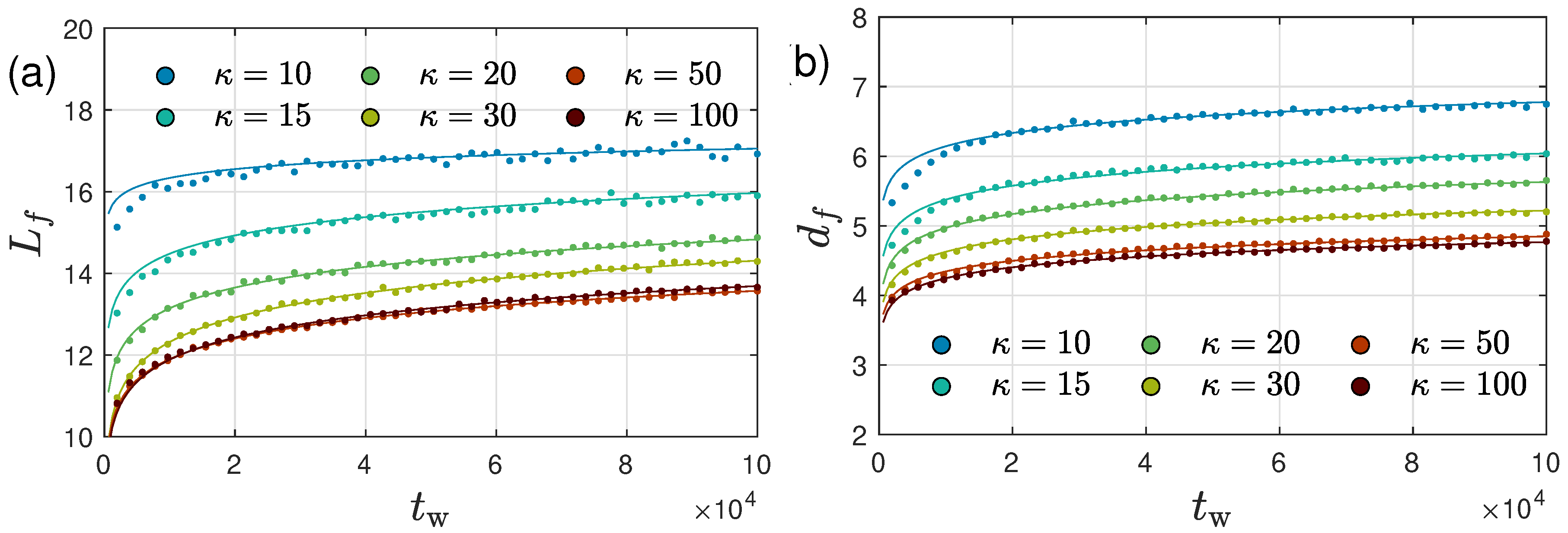
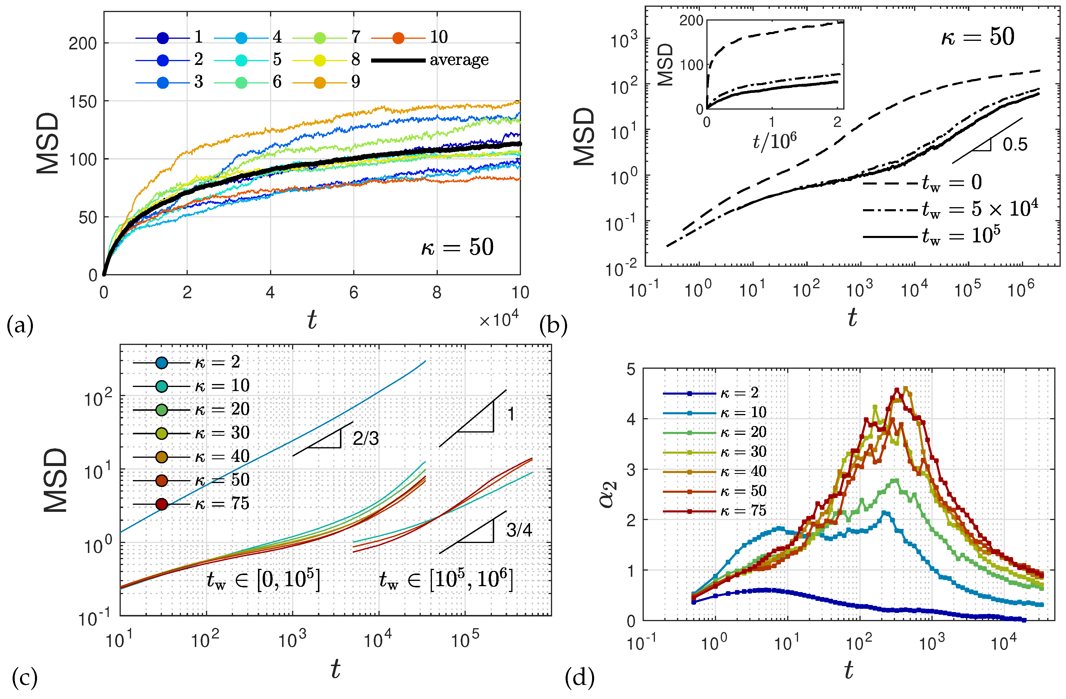
2.3. Ultra-Slow Coarsening and Self-Similarity

As we have seen in Sec. 2.2, various structural quantities show a weak dependence on the waiting time $t_{\mathrm{w}}$ since system preparation and do not seem to have fully reached steady state during the simulation time window. In this section we study this relaxation and the associated aging phenomenon more closely.

Figure 10 shows a sequence of snapshots for a typical system with $\kappa =50$ (see supplementary Figure S2 for corresponding snapshots for $\kappa =10$). The snapshots already suggest a coarsening of the network structure with increasing waiting time $t_{\mathrm{w}}$. To study the ongoing coarsening more quantitatively, we monitor the polymer surfaces and skeletons, as illustrated in Figure 11. We note that our polymer surfaces look rather similar to SEM or AFM images of biopolymers.[7,31,51,62,63] Figure 12(a), (b) and Figure 9(b) show the time evolution of the skeleton and surface-based characteristics, including the mean filament length $L_f$ and diameter $d_f$ and mean weighted chord length ${\ell }_1$ since system preparation, respectively. The very slow relaxation seen in Figure 3 can thus be attributed to an ultra-slow coarsening process of the network structure, as suggested by Figure 10 and Figure 11. Indeed, mass conservation arguments detailed in Sec. 4.6.4 suggest the scaling relation (1) to hold during late stages of coarsening, which we find to be satisfied to a good degree. Therefore, we conclude that coarsening mainly consists of filaments very slowly becoming thicker with pores very slowly getting larger.

We can monitor the ultra-slow coarsening also via the weighted chord length distribution of the dense phase, ${\mathcal{C}}_1$. As seen in Figure 9(c), (d), coarsening in the droplet and network-forming phase is associated with a slow shift of ${\mathcal{C}}_1$ to larger chord lengths, in agreement with the ultra-slow increase of the mean weighted chord length ${\ell }_1$ over time seen in Figure 9(b). The curves for $\kappa >10$ in Figure 9(b) are well reproduced (up to within 2%) by a logarithmic growth law (see Sec. 4.6.2). Extrapolating this law to a hypothetical final state of a single droplet or cylindrical filament would mean that ${\ell }_1$ keeps rising significantly up to times of the order of $t={10}^{15}$ to ${10}^{20}$! In other words, the mean ${\ell }_1$, if averaged over all times up to time $t_{\mathrm{end}}$, increases by about 15% if $t_{\mathrm{end}}$ is increased by one order of magnitude. Using ${\ell }_1\left(t\right)$ as a time-dependent characteristic length scale of the network, we can rescale ${\mathcal{C}}_1(s;t)$ at different times t onto a single master curve, ${\ell }_1\left(t\right){\mathcal{C}}_1(s;t)=f_1(s/{\ell }_1\left(t\right))$ (for details see supplementary Sec. 4.6.3). Figure 9(e) and (f) show the rescaled curves for different times t. A very good collapse of all data shown in Figure 9(c) and (d) onto a single master curve $f_1\left(x\right)$ is observed. The functional form of the universal master curve $f_1\left(x\right)$ for the network-forming phase is well represented by the analytical expression given in Eq. (29). Similar observations are made based on the weighted chord length distributions of the void space ${\mathcal{C}}_0$ (Figure 22). When scaled with the corresponding mean chord length of the void space ${\ell }_0\left(t\right)$, its master curve $f_0\left(x\right)$ is captured by the analytical expression (27). We can use the functional form of $f_0\left(x\right)$ to extrapolate ${\mathcal{C}}_0$ beyond the box size. This procedure allows us to estimate the moments of the distribution including the mean weighted and unweighted chord lengths, ${\ell }_0$ and $l_0$, free of finite-size effects.

Furthermore, we find that the scaled filament length $L_f/{\ell }_1$ and thickness $d_f/{\ell }_1$ as well as the scaled mean pore size $r_{\mathrm{pore}}/{\ell }_1$ are essentially time-independent when early stages of coarsening are discarded. Therefore, we conclude that the ultra-slow coarsening observed here is self-similar. A corresponding conclusion has recently been reached for a network-forming colloidal suspension based on the weighted chord length distribution ${\mathcal{C}}_0$ of the void spaces.[12]

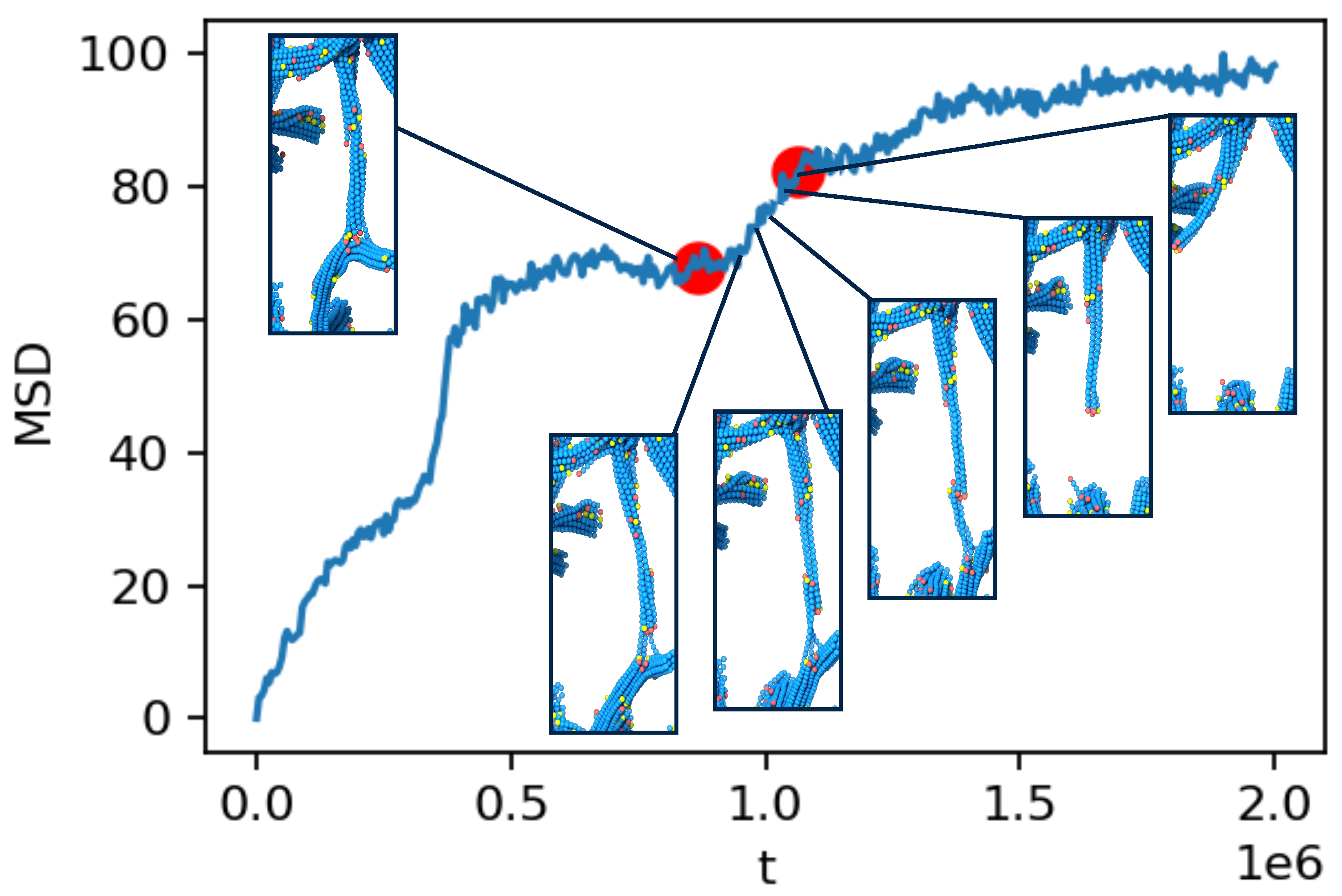
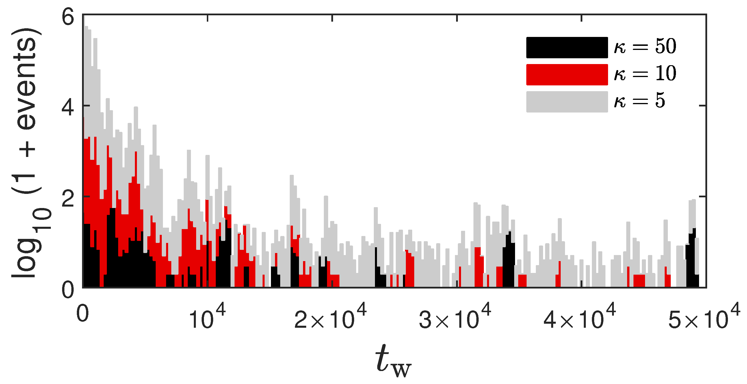
2.4. Coarsening Mechanism

In an effort to better understand the ultra-slow coarsening mechanism, we propose a minimal model of fibril breaking and rearrangement. See Figure 13 for a sketch. In this model, a representative fibril between two network junctions is modeled as a bundle of parallel chains that can diffuse longitudinally and independently of each other. The number of chains in the bundle is proportional to the fibril cross section. When all chain ends meet, the bundle breaks into two parts that each join a different fibril, leading to a corresponding increase in fibril cross sections. For fibrils with larger cross sections and correspondingly more chains, the probability that all chain ends meet is reduced and so is bundle breakage. This model predicts logarithmic growth for the mean number of chains in the cross-section of a fibril, Eq. (20), derived in Sec. 4.6.1. Therefore, the minimal model motivates the use of logarithmic growth laws to describe our data on coarsening. We find that logarithmic growth laws describe well not only the coarsening of the mean filament length and diameter as shown in Figure 12, but also other structural quantities such as the mean pore size, chord lengths, as well as pair and bending energies, with relative deviations of only a few percent. Some of these other quantities are shown together with fits to logarithmic growth laws in supplementary Figures S5, S6, and S7.

Coarsening of network structures has been observed in similar systems and described as either power-law[12] or logarithmic growth.[50] Power law and logarithmic behavior have been associated with two different universality classes of growth kinetics of activated processes, depending on whether the activation barriers grow (logarithmic) or do not grow (power law) with the domain size.[65] While the above arguments seem to favor logarithmic growth, we actually find that both families of fit functions provide equally good descriptions of our data. This indicates that our data do not allow to distinguish between the two universality classes of domain growth advocated in Ref.[65]. Furthermore, our systems do not exhibit the exponent 0.5 found in the power-law growth of characteristic pore sizes reported for the gas-liquid demixing of colloidal suspensions and simple fluids.[12] Instead, we observe a much weaker exponent of around 0.1 when fitting to power-law behavior. This finding might be taken as a further hint of non-universality of the ultra-slow coarsening kinetics and is in line with recent reports on non-universal aspects regarding the role of elasticity in polymer and colloidal gels.[53] Further investigations on universality classes in ultra-slow coarsening and limits thereof are left for future research.

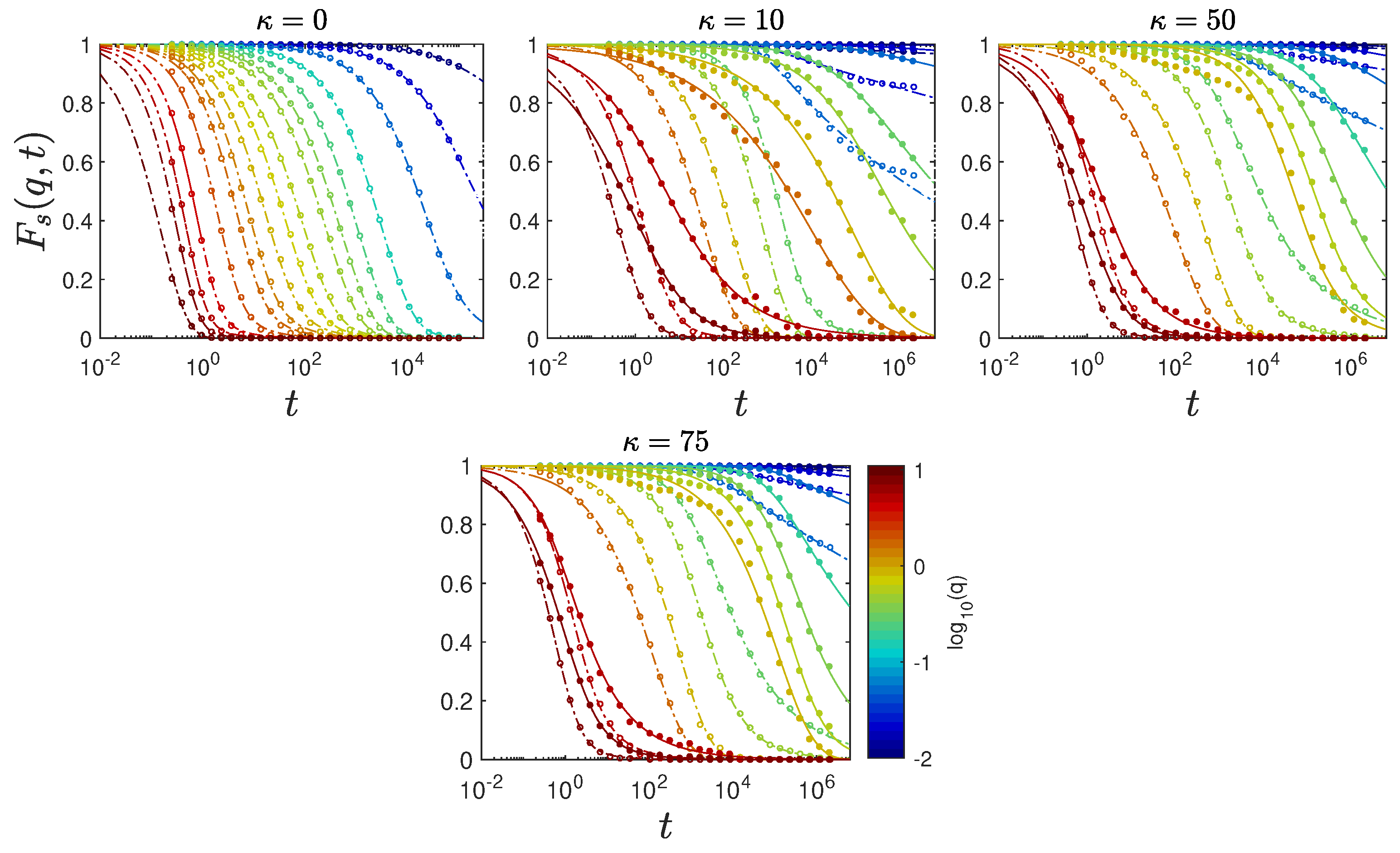
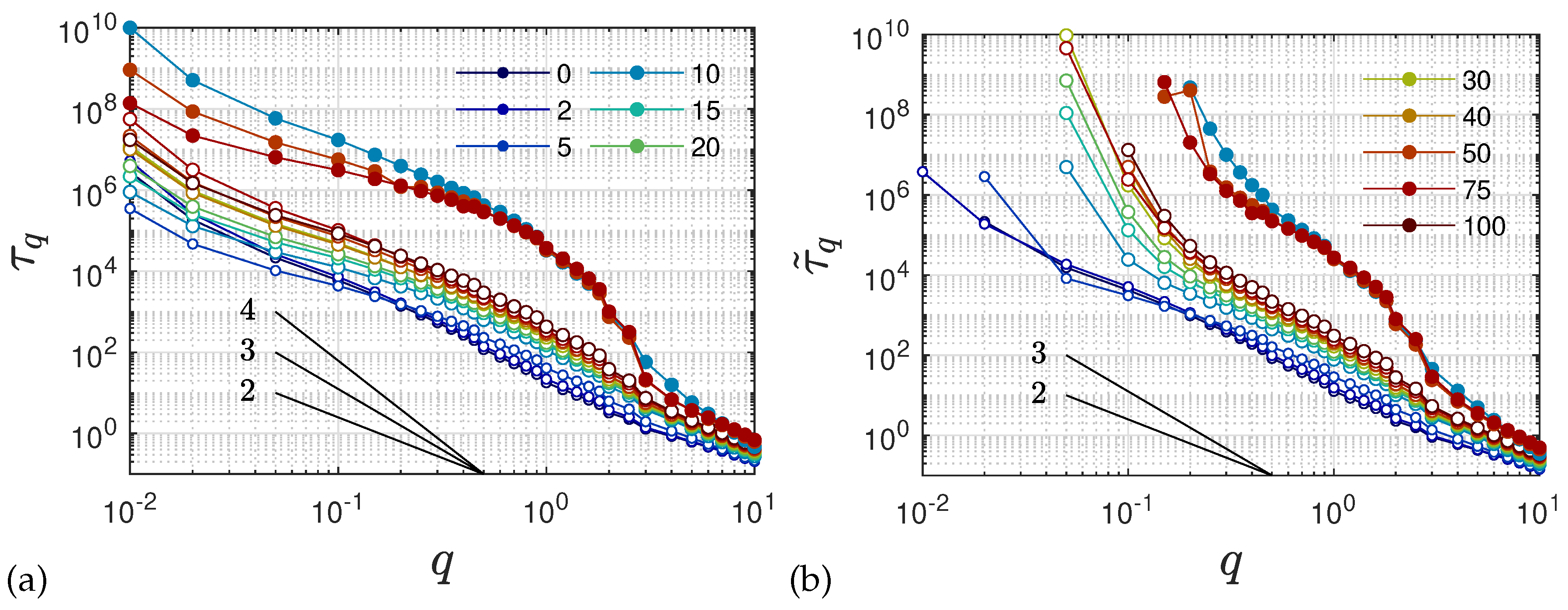
2.5. Anomalous Diffusion and Relaxational Dynamics

The enduring ultra-slow coarsening of these networks poses some challenges for the investigation of their dynamical properties. First and foremost, the lack of time-translational invariance since a stationary state has not been reached implies that we need to carefully distinguish dynamical properties at different waiting times $t_{\mathrm{w}}$ since preparation of the system.

As a first dynamic quantity we study the mean-square displacement (MSD) of bead positions $\Delta (t,t_{\mathrm{w}})=N_b^{-1}{\sum }_{j=1}^{N_b}{[{\mathbf{r}}_j(t+t_{\mathrm{w}})-{\mathbf{r}}_j\left(t_{\mathrm{w}}\right)]}^2$ as a function of time t since starting at a given waiting time $t_{\mathrm{w}}$. Figure 14(a) shows the exemplary case of $\Delta (t,0)$ for $\kappa =50$ and all 10 independent realizations of the system. For the corresponding $\Delta (t,{10}^5)$ up to $t={10}^6$ see supplementary Figure S1. Even though each system contains $N_b=30000$ beads, due to the absence of time-averaging, considerable sample-to-sample fluctuations are seen in Figure 14(a), supplementary Figure S1 and for other values of $\kappa$ (not shown). Closer inspection of trajectories reveals that, except for the relatively early stage ($t_{\mathrm{w}}\lesssim {10}^4$), filament fluctuations are rather small with correspondingly small bead displacements. At certain times, however, large reorganizations of the filament networks occur via filament breakage and subsequent re-attachment to another strand, leading to very large displacements in some parts of the network over a short time period. Figure 15 illustrates such a filament breaking event and the corresponding evolution of the MSD for an individual sample in the late stage of coarsening. Similar dynamic heterogeneities occur in a number of different systems, e.g. in glass-forming liquids[52] and aging colloidal gels.[17]

We will henceforth focus mostly on the ensemble-averaged MSD $\langle \Delta (t,t_{\mathrm{w}})\rangle$. Figure 14(b) shows $\langle \Delta (t,t_{\mathrm{w}})\rangle$ for $\kappa =50$ and three different values of $t_{\mathrm{w}}$. We note that the short-time ballistic regime is not visible on the scale shown in Figure 14(b). Instead, on a double-logarithmic scale, different diffusive regimes can be distinguished in Figure 14(b), all of them sub-diffusive on the time scale investigated. Moreover, the dynamics is found to be very slow with beads moving only a fraction of their diameter up to times $t\approx {10}^3$ except for the case $t_{\mathrm{w}}=0$. In the regime $t=5\times {10}^4$ up to $5\times {10}^5$, data seem to follow $\langle \Delta (t,t_{\mathrm{w}})\rangle \sim t^{0.5}$. In addition, a very significant dynamic slowing down is seen from 14(b) as the MSD decreases with increasing $t_{\mathrm{w}}$. Similar observations of waiting-time dependence and dynamic slowing down have been made for aging in colloidal gels.[17] At least on a qualitative level, the observed slowing down can in our case be linked to the coarsening network structure investigated above. Before investigating this relation further, we want to point out that ignoring the non-stationary nature of the networks and naively averaging over $t_{\mathrm{w}}$ can lead to wrong conclusions on the diffusive behavior of the system. As an example, Figure 14(c) shows $\langle \Delta (t,t_{\mathrm{w}})\rangle$ for various values of bending stiffness $\kappa$, averaged over rather large time intervals at an early $t_{\mathrm{w}}\in [0,{10}^5]$ and later stage $t_{\mathrm{w}}\in [{10}^5,{10}^6]$. In this case, the apparent MSD depends strongly on the chosen averaging interval. Moreover, with such averaging, significantly larger values of diffusion exponents are obtained that in some cases may even suggest normal diffusion. Similar artifacts due to inappropriate temporal averages in nonergodic systems are known and have been analyzed within continuous time random walk models with power-law distributed waiting times.[66]

We note that the dynamics observed here bears some similarities to the subdiffusive regime with MSD$\left(t\right)\sim t^{3/4}$ found in dilute and entangled solutions of semiflexible polymers.[67,68] For those systems, subdiffusive behavior occurs due to preferential fluctuations perpendicular to the chain contour for inner monomers at short times, before the MSD crosses over to normal diffusion at longer times when the MSD becomes comparable to the polymer size, MSD$\left(t\right)\approx \langle R^2\rangle$. For our systems, however, almost all chains are part of the temporary network, which leads to a severe hindrance of their mobility. As a consequence, the maximal values of MSD$\left(t\right)$ achieved over the duration of the simulations reported in Figure 14(c) remain an order of magnitude lower than $\langle R^2\rangle$. Also for the unpercolated system with $\kappa =2$, we observe a subdiffusive behavior MSD$\left(t\right)\sim t^{2/3}$, probably due to chain confinement within droplets as discussed in Sec. 2.2. Some of our observations may support the wormlike bundle model which predicts different dynamic regimes with the MSD perpendicular to the chain contour scaling first as $t^{3/4}$ then $t^{1/2}$ and again $t^{3/4}$, before ultimately approaching a plateau, as this model disregards filament rupture.[69]

To further characterize bead mobility, we refer to the non-Gaussian parameter ${\alpha }_2$ defined in Eq. (15). This quantity (Figure 14-d) characterizes deviations of bead displacements from a Gaussian distribution. For unpercolated systems ($\kappa =2$), ${\alpha }_2$ remains small and approaches zero relatively quickly. For percolated systems on the other hand, ${\alpha }_2$ reaches peak values between 4 and 5 for $\kappa \ge 30$ over an extended period of time around $t\approx {10}^2\dots {10}^3$ before the system enters a different diffusive regime. For larger $t_{\mathrm{w}}$, the peak height of the non-Gaussian parameter grows and moves to later times. Similar peaks in the non-Gaussian parameter have been observed in other systems such as supercooled liquids and glass-forming flexible polymers. In those systems, the peaks in ${\alpha }_2$ occur near the end of the plateau region of the MSD and have been associated with dynamic heterogeneities due to collective relaxation phenomena such as “cage breaking”.[70] Here, however, the peak values observed in ${\alpha }_2$ are much larger, indicating much stronger deviations from a Gaussian distribution. In addition, although Figure 14(b) indicates very slow, sub-diffusive dynamics, the MSD is still increasing and does not really plateau at intermediate times. These results are more similar to those found in network liquids[71] and suggest that there are different relaxation mechanisms at work in these percolated networks compared to glassy dynamics, in agreement with recent conclusions.[53] For intermediate values of the bending stiffness at the onset of a percolated network ($\kappa =10$), an additional peak in ${\alpha }_2$ is seen from Figure 14(d). In polymer melts composed of rather rigid chains, the onset of a second peak was seen in computer simulation studies of a model system similar to the one considered here.[72] These authors assumed slow relaxation of nematic domains as the underlying mechanisms of the second peak at late times. Such explanations probably do not carry over to the present case where we observe an additional peak in ${\alpha }_2$ at earlier times. A double peak in ${\alpha }_2$ was also seen in computer simulations for a particular choice of parameters in a model for microemulsions, and related to the difference between local cage-breaking versus bond relaxation events.[73]

The self part of the intermediate scattering function, $F_s(q,t)$, defined in Eq. (14) provides more information on the length-scale dependent relaxational dynamics. See Sec. 4.4 for more details on this quantity, and supplementary Sec. S1 for a visualization of contributions to $F_s(q,t)$. Figure 16 shows $F_s(q,t)$ for several (color coded) values of the wave number q over a similar range to those investigated for the static structure factor $S_{\mathrm{sc}}\left(q\right)$ in Figure 4. For better visibility, only a tiny fraction of the simulation data are shown as circles in this plot (full datasets available in supplementary Figure S13). On small length scales below the bead diameter, i.e. $q\gtrsim 6$, relaxation occurs relatively fast and is not much affected by the bending stiffness $\kappa$. On the length scales of the end-to-end distances R of the polymers, corresponding to $q_{\mathrm{ee}}=2\pi /R$, the relaxation of $F_s(q_{\mathrm{ee}},t)$ is generally faster than the orientational end-to-end vector relaxation (see supplementary Figure S8), indicating the importance of cooperative effects on these length scales (including the formation locally aligned chains in droplets and bundles). For all systems investigated, relaxation is slowing down by orders of magnitude with decreasing q corresponding to larger length scales. Except for $\kappa =0$, each panel in Figure 16 shows two sets of data corresponding to waiting times $t_{\mathrm{w}}=0$ and $t_{\mathrm{w}}={10}^5$. Relaxation slows down with increasing waiting time, consistent with our observation of dynamic slowing down of the MSD. Such behavior is typical for aging, especially in glassy systems.[74,75] The slowing with increasing $t_{\mathrm{w}}$ is particularly strong for small q values ($q<1$), where the intermediate scattering function does not relax to zero on the time scale of the simulations (and would not do so for $q\ll 1$ even if we were to increase the simulation time window by many orders or magnitude). Therefore, we deal with an effective aging and non-ergodic system. This non-ergodic behavior is not only common in colloidal systems with infinite lifetime of bonds, [73] but also reported for real transient networks of semiflexible polymers.[1]

To discuss the relaxation dynamics more quantitatively, we fit the $F_s(q,t)$ simulation data using the "power-ML" function

$${\tilde{F}}_s(q,t)={\left[E_{\beta }(-{(t/{\tau }_q^{\prime })}^{\beta })\right]}^{\alpha /\beta },{\tau }_q^{\prime }={\left({\displaystyle \frac{\alpha }{{\beta }^2\Gamma \left(\beta \right)}}\right)}^{1/\beta }{\tau }_q,$$

(2)

where $E_{\beta }\left(z\right)={\sum }_{n=0}^{\infty }{z}^n/\Gamma (1+\beta n)$ denotes the Mittag-Leffler function and $\Gamma \left(x\right)$ the Gamma function. For the special case $\alpha =\beta$, Eq. (2) reduces to the standard Mittag-Leffler function $E_{\beta }(-{(t/{\tau }_q^{\prime })}^{\beta })$ which is discussed in the literature as the solution to a linear fractional differential equation.[76] By construction, we impose non-negative $E_{\beta }$, i.e. we restrict the fits to $\beta \in [0,1]$. With two exponents $\alpha ,\beta$ and an effective relaxation time ${\tau }_q$, our simulation data for $t_{\mathrm{w}}=0$ and all values of $\kappa$ and q investigated and over seven orders of magnitude in t can be fitted very well by the power-ML function (2), as shown by the close agreement between the lines and open symbols in Figure 16. For the $t_{\mathrm{w}}={10}^5$ data (filled symbols) Eq. (2) does not capture all details in the intermediate time and q ($q\approx 1$) regime.

For relatively early times, $t\ll {\tau }_q^{\prime }$, the power-ML function ${\tilde{F}}_s$ describes a stretched exponential decay $exp[-{(t/{\tau }_q)}^{\beta }]$, frequently employed to fit relaxation in gels and glasses.[17,73] The corresponding values of the stretching exponents $\beta$ are shown for $t_{\mathrm{w}}=0$ in Figure 17(b). A stretching exponent $\beta =3/4$ was theoretically predicted for solutions of semiflexible polymers.[77] Here we observe a rather large range of $\beta \in [0.6,1]$ values that moreover vary non-monotonically with the wave vector q. Note that similar values of $\beta$ but in a smaller range $[0.6,0.75]$ are found if a stretched exponential function is used to fit $F_s(q,t)$ for all times. Those results are not shown since the quality of the corresponding fits is generally inferior to those by the power-ML function. For our model system we can rule out compressed exponential relaxation[17] not only because the power-ML (2) does not allow to capture the $\beta >1$ regime, but also since $t(d/dt)[ln(-ln{F}_s(q,t))]$ does not exceed unity for our measured data, for both $t_{\mathrm{w}}=0$ and $t_{\mathrm{w}}={10}^5$. From a second-order cumulant expansion, $F_s(q,t)\approx exp[-(q^2/6)\langle \Delta (t,t_{\mathrm{w}})\rangle ](1+\mathcal{O}\left(q^4\right))$, the short-time, small wave vector limit is related to the mean-square diffusion studied above. Our numerical data satisfy this relation (not shown).

For times $t\gg {\tau }_q^{\prime }$, the power-ML function (2) smoothly interpolates to a power-law behavior, ${\tilde{F}}_s\sim t^{-\alpha }$, with $\alpha \ne \beta$ in general. Such pronounced power-law behavior is seen in Figure 16, in particular for small q values. The power-law exponent $\alpha$ obtained from fits to Eq. (2) is shown in Figure 17(a). While for $q\gtrsim 5$, $F_s(q,t)$ decays relatively rapidly so that the behavior is dominated by a stretched-exponential relaxation, relaxation slows down significantly for $q\lesssim 1$ and the power-law regime becomes more and more dominant. Most strikingly, we find that in this regime the $\alpha$ decreases towards zero with decreasing q. While the values of $\alpha$ vary significantly with $\kappa$ for $t_{\mathrm{w}}=0$, only small variations are seen for $t_{\mathrm{w}}={10}^5$, where approximately $\alpha \sim q^{6/5}$ for $q<1$ (supplementary Figure S11-b). Therefore, the long-time relaxation becomes slower and slower on larger scales as the exponent decreases towards zero.

Having clarified short and long-time relaxation regimes, we now turn to a discussion of the characteristic relaxation times. Figure 18(a) shows the relaxation time ${\tau }_q$ of the power-ML function (2) governing the time scale of the stretched exponential relaxation. In addition, Figure 18(b) shows an alternative definition of a relaxation time ${\tilde{\tau }}_q$ which characterizes the decay of $F_s(q,t)$ to a prescribed level. For convenience we here choose $F_s(q,{\tilde{\tau }}_q)=1/2$. For those cases where the simulation data of $F_s(q,t)$ do not decay below $1/2$, we use extrapolations from Eq. (2) to determine ${\tilde{\tau }}_q$. While the numerical values of ${\tau }_q$ and ${\tilde{\tau }}_q$ are different, both characteristic relaxation times show qualitative similar behavior at large q. First, for $t_{\mathrm{w}}=0$ (open symbols in Figure 18), the relaxation times show approximately a scaling $q^{-2}$ for $q\gtrsim {10}^{-1}$ and the relaxation times are increasing with increasing bending stiffness $\kappa$. Aged systems with $t_{\mathrm{w}}={10}^5$, however, show a rather abrupt increase of ${\tau }_q,{\tilde{\tau }}_q$ by about three orders of magnitude when q decreases from $q\approx 3$ to $q\approx 2$. Interestingly, ${\tau }_q,{\tilde{\tau }}_q$ are rather insensitive to the precise value of $\kappa$ in the network-forming regime over a relatively large interval of q vectors. Figure 18 demonstrates a very rich relaxation behavior of the system that moreover changes significantly between initial ($t_{\mathrm{w}}=0$) and aged ($t_{\mathrm{w}}={10}^5$) samples. Not only do large structures relax more slowly in these systems, they do so in a particular manner with a $\kappa$-independent onset at a characteristic wave number $q_{\mathrm{c}}$. With $q_{\mathrm{c}}\approx 2\dots 3$, this length scale roughly corresponds to the filament radius $d_f/2$. With relaxation times exceeding ${10}^6\dots {10}^8$ for $q<{10}^{-1}$ by far, these systems show ultra-slow relaxation alongside the coarsening behavior established above.

3. Conclusions

We use comprehensive molecular simulations of a generic coarse-grained model to study semiflexible polymers where cohesive interactions lead to physical, reversible crosslinks. Polymers are found to self-assemble into droplets for weak bending stiffness, i.e. for relatively flexible chains. For more rigid chains, on the other hand, the interplay between attractive interactions with periodic boundary conditions results in the formation of percolated networks of filaments – a typical behavior observed in many biopolymers.

The static structure factor shows a pronounced $q^{-4}$ Porod regime at intermediate scattering vectors q, signaling the presence of well defined interfaces. From a skeleton analysis, we find that the network is dominated by three-fold junctions, with four- or higher-order junctions and dangling ends accounting for a tiny fraction only. We identify the links between junctions as filaments and observe that their mean thickness decreases monotonically with increasing persistence length, in agreement with previous simulation studies,[45] but in contrast with results from scattering experiments on PEG-grafted methylcellulose chains.[22] The resolution of this conundrum is left for future research. We determine the pore size and chord length distribution used to define typical mesh sizes. We find characteristic scaling laws for these systems so that e.g. the mean pore radius and the mean filament thickness are proportional to one another.

Besides the static structure, we also investigate dynamic properties of the systems at different waiting times since system preparation. Generally, we observe different dynamic regimes of slow, sub-diffusive dynamics with strongly non-Gaussian displacements over a broad time window. In addition, dynamic slowing down is observed as the system ages. The underlying reason for the anomalous diffusion are dynamical heterogeneities due to rare reorganizations of the filament networks with large cooperative displacements of a significant number of beads. The relaxation dynamics is therefore intermittent and dominated by individual events of filament breaking and recombining that become more rare as the system coarsens (Figure 19). These dynamical heterogeneities are also reflected by stretched exponential and power-law relaxation of the incoherent scattering function, with substantial dynamical slowing down as the system relaxes further. It is important to remark that the incoherent scattering function in the small wave number regime does not decay to zero on the time scale of our simulations. The corresponding lack of ergodicity since large-scale structure are not fully equilibrated has been pointed out also in experiments on gels of amyloid fibers.[1]

We observe a logarithmic dependence on waiting time since system preparation for structural and thermodynamic quantities. This weak logarithmic dependence is easily overlooked when monitoring these quantities on linear scales as is usually done to check for stationarity. Also some quantities like the static structure factor and gyration radius are less sensitive to the ultra-slow relaxation (see Figure 3 and supplementary Figure S7). For other, in particular dynamic, quantities, however, the waiting-time dependence is significant and naive averaging can lead to incorrect conclusions, e.g. regarding the diffusive behavior.

From the logarithmic coarsening laws we can estimate necessary waiting times needed for quantities of interest to change less than a given tolerance. Although one needs to be very cautious with such extrapolations, the ultra-slow logarithmic relaxation would prevent us from reaching a (approximate) stationary state even with a massive increase in computational resources. Network formation in similar systems has been interpreted as interfering with spinodal decomposition and leading to kinetic arrest. The enduring relaxation can be interpreted as an aging process where the system explores lower and lower potential (bond and bending) energy minima. Structurally, for our system this aging phenomenon involves an ultra-slow coarsening process of network structures where filaments very slowly become thicker while pores become larger. Since both length scales are intimately linked, the ultra-slow coarsening is self-similar in the course of time as evidenced by the very good data collapse onto master curves of the chord length and pore size distributions. It would be interesting to compare these findings with experimental results on aging in comparable biopolymer networks. Exploring the interplay of aging and coarsening with viscoelastic properties of these networks is left for future research.

4. Materials and Methods

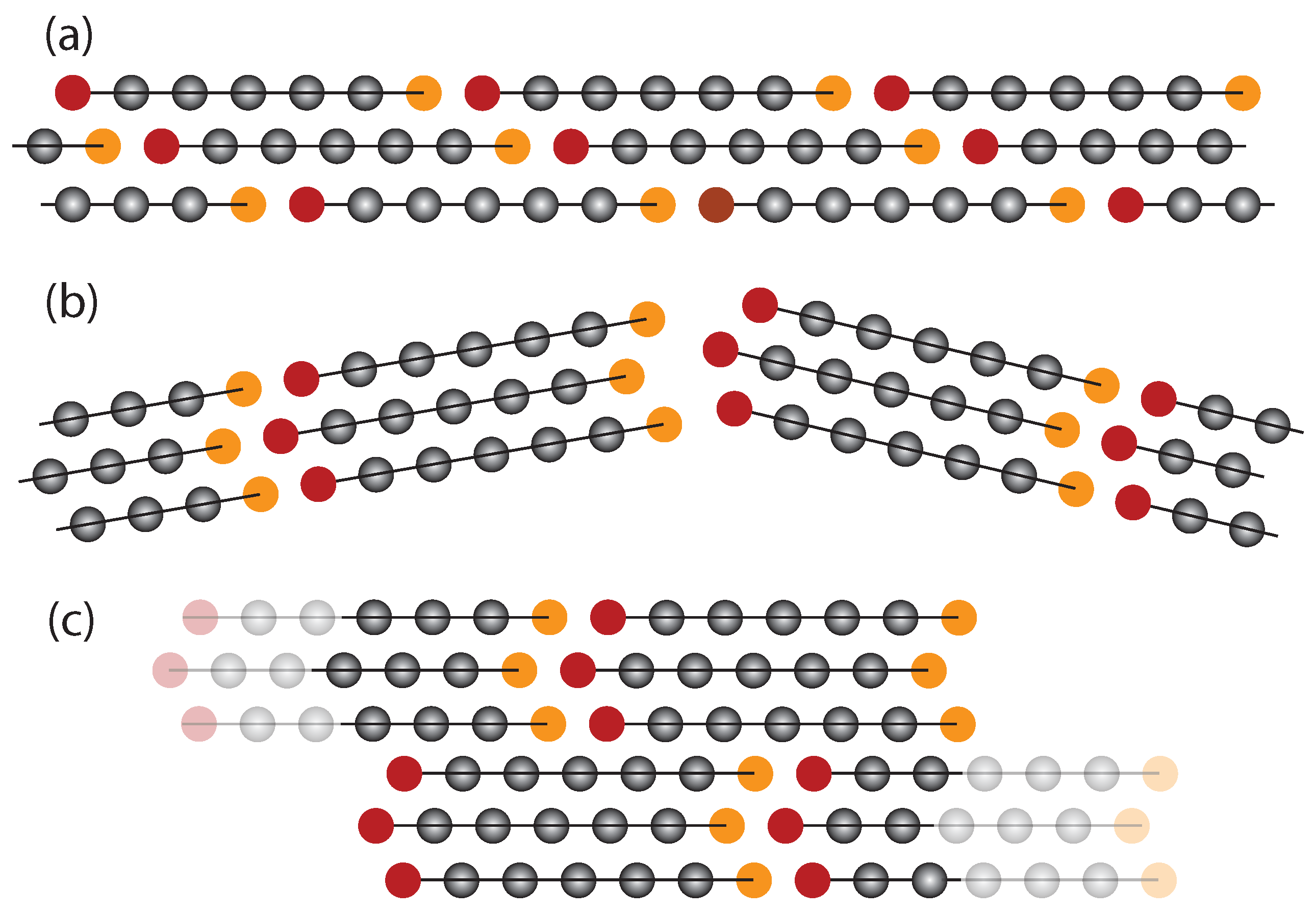
4.1. Coarse-Grained Simulation Model

The model studied here is a semiflexible, anharmonic multibead-spring model that differs from the celebrated KG model [35] for linear polymer chains in melts only with respect to bending energy and interaction cutoff, and is conveniently implemented using LAMMPS[78] (script available in Sec. S8).

4.1.1. Model Equations and Parameters

The usually $N_c=1000$ linear, monodisperse bead-spring chains, each consisting of $N=30$ identical beads, $N_b=N_{c}N$ beads in total, are contained in a periodic simulation box with volume V, at bead number density $\rho =N_b/V$ and temperature $T=1$. All permanently bonded beads along the linear chains interact via the radially symmetric finitely extendable nonlinear elastic (FENE) potential,[79]

$$U_{\mathrm{FENE}}\left(b\right)=-{\displaystyle \frac{k}{2}}{R}_0^{2}ln[1-{(b/R_0)}^2],$$

(3)

with spring coefficient $k=30$ and maximum extension $R_0=1.5$, where b denotes a bond length. This potential serves as a rather poor approximation to the inverse Langevin function at large extensions,[80] but is typically employed. All pairs of beads interact via a truncated, radially symmetric Lennard-Jones potential,

$$U_{\mathrm{LJ}}\left(r\right)=4{ϵ}_b(r^{-12}-r^{-6}-r_c^{-12}+r_c^{-6}),r\le r_c,$$

(4)

and $U_{\mathrm{LJ}}\left(r\right)=0$ for $r>r_c$, where ${ϵ}_b=1$ and $r_c=r_{\min }=2^{1/6}$ for all permanently bonded beads, ${ϵ}_b=3$ for all nonbonded beads, while $r_c$ for all nonbonded beads remains a model parameter. In Eq. (4), $r=|{\mathbf{r}}_i-{\mathbf{r}}_j|$ denotes a spatial distance between a pair of beads i and j. A pair of nonbonded beads can be regarded as having formed a temporary (reversible) bond as long as the distance between the two beads is below $r_c$. The energy penalty to break such a temporary bond defines a cohesion energy

$$E_{\mathrm{coh}}=-U_{\mathrm{LJ}}\left(r_{\min }\right)={\displaystyle \frac{{(2-r_c^6)}^2{ϵ}_b}{r_c^{12}}}$$

(5)

that ranges between zero and ${ϵ}_b=3$, depending on the choice of $r_c$. Equation (5), employing ${ϵ}_b=3$, can also be inverted as $r_c={[6/(3-\sqrt{3E_{\mathrm{coh}}})]}^{1/6}$.

Finally, each triplet of adjacent permanently bonded beads interacts via the cosine bending potential[36,37,38]

$$U_{\mathrm{bend}}=\kappa (1-{\mathbf{u}}_i·{\mathbf{u}}_{i+1})$$

(6)

where the bending stiffness $\kappa$ is a key model parameter, and ${\mathbf{u}}_i={\mathbf{b}}_i/b_i$ (with ${\mathbf{b}}_i={\mathbf{r}}_{i+1}-{\mathbf{r}}_i$) is a unit bond vector, if beads i and $i+1$ are permanently bonded to each other. Since $T=1$ and $k_{\mathrm{B}}=1$, $\kappa /k_{\mathrm{B}}T=\kappa$ in our case, and we write $\kappa /k_{\mathrm{B}}T$ only if it serves to highlight a dependency on temperature. The summed bond vectors of an individual chain are identical with the chain’s end-to-end vector $\mathbf{R}={\sum }_{i=1}^{N-1}{\mathbf{b}}_i$.

4.1.2. Preparation of Model Systems

Systems are generated by placing $N_c$ semiflexible chains with initial bond length $b_{\mathrm{init}}=1$ and with persistence length $L_p=-b_{\mathrm{init}}/ln\left[\mathcal{L}(\kappa /k_{\mathrm{B}}T)\right]$, involving the Langevin function $\mathcal{L}\left(x\right)=coth\left(x\right)-x^{-1}$, but without overlap (minimum bead-bead distance 0.85)[81] into a periodic simulation box whose volume is determined by either (i) an initial bead number density ${\rho }_{\mathrm{init}}=0.02$ for the NPT ensemble, or (ii) ${\rho }_{\mathrm{init}}=0.05$ for the NVT ensemble simulations. The equations of motion resulting from the mentioned potentials are then integrated using classical thermo- and barostats (NPT only) using an integration time step $\Delta t=0.005$. For case (i) the system is equilibrated within the NPT ensemble until its pressure is fluctuating about zero; at this time the system has reached a number density $\rho$ that may largely deviate from ${\rho }_{\mathrm{init}}$, and is moreover insensitive to ${\rho }_{\mathrm{init}}$ due to the relatively low ${ϵ}_b=3$ that we have chosen. The simulations within the NPT ensemble suggest to use $\rho =0.05$ for the NVT ensemble simulation. Here, for case (ii), the short relaxation stage (duration ${10}^3$) is followed by a measurement stage of duration ${10}^5$. Long runs up to $t_{\mathrm{w}}=2.1\times {10}^6$ were performed for $\kappa \in \{10,50,75\}$. The begin of the measurement stage defines waiting time $t_{\mathrm{w}}=0$. During these stages, we keep $\rho$ fixed, and integrate the equations of motion using a Langevin thermostat with friction coefficient $\zeta =0.5$, following previous works.[35,82]Supplementary movies E to G and E+ to G+ show selected systems during the short relaxation and early measurement stage, and during the coarsening stage, respectively.

4.2. Static Structure Factors

The static structure factor $S\left(\mathbf{q}\right)$ is defined by

$$S\left(\mathbf{q}\right)={\displaystyle \frac{1}{N_b}}\sum _{i,j=1}^{N_b}\langle e^{i\mathbf{q}·({\mathbf{r}}_i-{\mathbf{r}}_j)}\rangle ={\displaystyle \frac{1}{N_b}}\langle |\delta {\rho }_{\mathbf{q}}{|}^2\rangle ,$$

(7)

where the double sum runs over all $N_b$ beads in the system and $\delta {\rho }_{\mathbf{q}}={\sum }_{j=1}^{N_b}{e}^{i\mathbf{q}·{\mathbf{r}}_j}$ are the Fourier modes of the fluctuating density field. The angular brackets denote ensemble averaging. For isotropic systems, S depends only on the modulus $q=\left|\mathbf{q}\right|$ of the wave vector, and can be used to calculate the pair correlation function $g\left(r\right)=1+{\left(2{\pi }^{2}nr\right)}^{-1}{\int }_0^{\infty }qsin\left(qr\right)[S\left(q\right)-1]dq$. We efficiently evaluate $S\left(q\right)$ via numerical Fourier transform on a $2^{12}\times 2^{12}$ grid to prevent evaluating a double sum or the pair correlation function at large distances (we find that smaller grids lead to inaccurate results in the vicinity of the first minimum of $S\left(q\right)$ at about $q=\pi$). The smallest wave vector $q_{\min }=2\pi /L_x$ that we can meaningfully study corresponds to the largest length scale of our system which is the linear size $L_x=V^{1/3}$ of the cubic simulation box. The largest $q_{\max }=4096q_{\min }$ is determined by the chosen grid.

We also evaluate the isotropic scattering function of an individual chain, defined by the Fourier-transformed intra-molecular radial pair correlation function[83]

$$S_{\mathrm{sc}}\left(q\right)={\displaystyle \frac{1}{N}}\sum _{i,j=1}^N\langle e^{i\mathbf{q}·({\mathbf{r}}_i-{\mathbf{r}}_j)}\rangle =1+{\displaystyle \frac{2}{N}}\sum _{i,j>i}^N〈{\displaystyle \frac{sin\left(q{r}_{ij}\right)}{q{r}_{ij}}}〉$$

(8)

where the double sum runs over all beads of a given chain and the ensemble average includes an average over all chains. By its definition, $S_{\mathrm{sc}}\left(0\right)=1+(N^2-N)/N=N$. Since $N\ll N_b$, the double sum in Eq. (8) can be evaluated directly, and there is no need to calculate the radial pair correlation function. Since unfolded bead coordinates are used, the box size does not limit the range of possible q values, and $S_{\mathrm{sc}}\left(q\right)$ can be evaluated down to $q=0$ for any box size $L_x$. The quantity $S_{\mathrm{sc}}\left(q\right)$ for continuous wormlike-chain with and without excluded volume had been studied theoretically.[84,85]

For discrete WLCs in the absence of excluded volume effects, $S_{\mathrm{sc}}$ can be calculated (i) recursively via the Laplace-transformed moments of the end-to-end distribution function, [86,87] or (ii) numerically upon generating an ensemble of discrete WLCs, or (iii) analytically using one of the existing approximations for the radially symmetric distribution function $f(L,L_p;R)$ for the end-to-end distance R of a discrete WLC with contour length L and persistence length $L_p$. We here employed the two latter approaches: (ii) To generate an ensemble of $N_c$ discrete WLC with given N, b and $\kappa /k_{\mathrm{B}}T$ or $L_p=-b/ln\left[\mathcal{L}(\kappa /k_{\mathrm{B}}T)\right]$ we grow each chain bond by bond, choose bond vector ${\mathbf{b}}_{j+1}=z{\mathbf{b}}_j+b\sqrt{1-z^2}(\mathbf{u}\times {\mathbf{b}}_j)/|\mathbf{u}\times {\mathbf{b}}_j|$ with $z=-1+ln(1+c\xi )k_{\mathrm{B}}T/\kappa$, $\xi$ a random number equally distributed on the interval $[0,1]$, $\mathbf{u}$ a random unit vector, and $c=e^{2\kappa /k_{\mathrm{B}}T}-1$. This algorithm follows from the known distribution of bond angles for the discrete WLC. For huge $\kappa /k_{\mathrm{B}}T>100$, to prevent numerical precision problems, $z=\max (-1,1+ln\left(\xi \right)k_{\mathrm{B}}T/\kappa )$ can be employed instead of the above exact expression. The bead positions, given by ${\mathbf{r}}_i={\mathbf{r}}_{i-1}+{\mathbf{b}}_i$, are then directly used to evaluate Eq. (8). For approach (iii), we start from the highly accurate analytic expression for $f(L,L_p;R)$ proposed by Becker et al.,[88] subsequently normalized so that $\int f(L,L_p;R)d^{3}R=1$, and then evaluate the intramolecular pair correlation function $g_{\mathrm{sc}}\left(r\right)$ by summing over all partial contour distances, i.e., $g_{\mathrm{sc}}\left(r\right)=N^{-1}{\sum }_{j=1}^N(N-j)f(jb,L_p;r)$. With $g_{\mathrm{sc}}\left(r\right)$ at hand, we evaluate $S_{\mathrm{sc}}\left(q\right)=1+4\pi q^{-1}{\int }_0^{L}rsin\left(rq\right)[g_{\mathrm{sc}}\left(r\right)-g_{\mathrm{sc}}\left(L\right)]dr$ with $L=(N-1)b$. For the large $L_p>Nb$, approach (iii) runs into numerical problems and we rely on (ii). Both approaches (ii) and (iii) allow us to consider variable bond lengths b, but we find that our measured $S_{\mathrm{sc}}\left(q\right)$ is already well captured over the whole q range including the peaks for $q\gg b^{-1}$, by using a fixed value $b=1$. As a side-result, we have access to $g_{\mathrm{sc}}\left(r\right)$ without having to measure this quantity directly.

4.3. Effective Persistence Lengths

We implemented two approaches to extract effective persistence lengths ${\ell }_p$ and $L_p$ from chain configurations. In the "local" approach, we use the mean bending energy per atom $e_a$, usually reported by LAMMPS (eangle). The corresponding ${\ell }_p$ is then given by ${\ell }_p=-b/ln\langle {\mathbf{u}}_i·{\mathbf{u}}_{i+1}\rangle$ with $\langle {\mathbf{u}}_i·{\mathbf{u}}_{i+1}\rangle =1-N{e}_a/\left[(N-2)\kappa \right]$. In the second "global" approach we use the ratio between mean squared end-to-end distance $\langle R^2\rangle$ and squared radius of gyration $R_g^2$ of the N-chains (supplementary Figure S10) and estimate an effective persistence length $L_p$ assuming that the individual chains exhibit the statistics of a discrete WLC (Figure 20). To this end let us recall the exact analytic expressions for a discrete WLC with $N-1$ bonds and contour length $L=(N-1)b$,81]

$$\begin{array}{ccc}\hfill {\displaystyle \frac{\langle R^2\rangle }{bL}}& =& {\displaystyle \frac{1+z}{1-z}}-{\displaystyle \frac{2z(1-z^{N-1})}{(N-1){(1-z)}^2}},\hfill \\ \hfill {\displaystyle \frac{6R_g^2}{bL}}& =& \left[{\displaystyle \frac{1+z}{1-z}}-{\displaystyle \frac{6z}{(N-1){(1-z)}^2}}\right]{\displaystyle \frac{N+1}{N}}\hfill \end{array}$$

(9)

$$\begin{array}{ccc}& & +{\displaystyle \frac{12z[N-z(N+1)+z^{N+1}]}{{(1-z)}^4(N-1)N^2}},\hfill \end{array}$$

(10)

with $z=e^{-b/L_p}$. Note that the ratio $\langle R^2\rangle /R_g^2$ does depend on $L_p$ only. For $N\gg 1$ and $L_p\gg b$, the discrete WLC converges to the better known continuous WLC characterized by [89]

$$\begin{array}{ccc}\hfill {\displaystyle \frac{\langle R^2\rangle }{2L_{p}L}}& =& {\displaystyle \frac{L}{2L_p}}{f}_{\mathrm{Debye}}(L/L_p),\hfill \end{array}$$

(11)

$$\begin{array}{ccc}\hfill {\displaystyle \frac{6R_g^2}{2L_{p}L}}& =& 1-{\displaystyle \frac{3L_p}{L}}[1-f_{\mathrm{Debye}}(L/L_p)],\hfill \end{array}$$

(12)

with the Debye function $f_{\mathrm{Debye}}\left(x\right)=2(e^{-x}+x-1)/x^2$. In contrast to the continuous WLC, the discrete WLC correctly captures dumbbells, as $\langle R^2\rangle =b^2$ and $R_g^2=b^2/4$ for $N=2$. For $\kappa /k_{\mathrm{B}}T\gg 1$ or $L_p/b\gg 1$, $L_p/b\approx \kappa /k_{\mathrm{B}}T$. For an ideal WLC the local ${\ell }_p$ (obtained from $e_a$) and global $L_p$ (obtained from $\langle R^2\rangle$, $R_g^2$, or their ratio) are identical, and ${\ell }_p=L_p=L_p^{\mathrm{WLC}}$ with $L_p^{\mathrm{WLC}}=-b/ln\left[\mathcal{L}(\kappa /k_{\mathrm{B}}T)\right]$.

Note that expressions (9) and (10) were written differently, but equivalently, in the mentioned Ref.[81]. With the nonzero components $A_{13}=-(\pi /2)I_1(L_p/b)/sinh(L_p/b)$ and $A_{33}=z$ of a $3\times 3$ matrix $\mathbf{A}$, involving the modified Bessel function $I_1$ of the first kind, the mean squared end-to-end distance was left un-evaluated in terms of $\mathbf{A}$ as $\langle R^2\rangle /bL=C_{\infty }-[2/(N-1)]{[\mathbf{A}·(\mathbf{1}-{\mathbf{A}}^{N-1})·{(\mathbf{1}-\mathbf{A})}^{-2}]}_{33}$, where $C_{\infty }=[(\mathbf{1}+\mathbf{A})·{(\mathbf{1}-{\mathbf{A}}^{-1}]}_{33}$.

4.4. Intermediate Scattering Function $F(q,t)$

Letting ${\mathbf{r}}_j\left(t\right)$ denote the coordinates of the jth bead at time t, the intermediate scattering function (also known as dynamic structure factor) is defined by

$$F(\mathbf{q},t)={\displaystyle \frac{1}{N_b}}\langle \delta \rho (\mathbf{q},t+t_{\mathrm{w}})\delta \rho (\mathbf{q},t_{\mathrm{w}})\rangle ,$$

(13)

with $\delta \rho (\mathbf{q},t)={\sum }_{j=1}^{N_b}exp[i\mathbf{q}·{\mathbf{r}}_j\left(t\right)]$ the instantaneous density fluctuation at wave vector $\mathbf{q}$. For $t=0$, Eq. (13) reduces to the static structure factor $F(\mathbf{q},0)=S\left(\mathbf{q}\right)$ introduced in Eq. (7).

We evaluate the radially symmetric self-part of $F(\mathbf{q},t)$,[90] $F_{\mathrm{s}}(q,t)=\langle exp[i\mathbf{q}·({\mathbf{r}}_j(t+t_{\mathrm{w}})-{\mathbf{r}}_j\left(t_{\mathrm{w}}\right))]\rangle$, for a selected number of q values. The average is taken over trajectories of 10 statistically independent starting configurations, and all $\mathbf{q}$-vectors with length $q=\left|\mathbf{q}\right|$. Such integrals over the unit sphere of orientations of $\mathbf{q}$ vectors amounts to evaluating

$$F_{\mathrm{s}}(q,t)=〈{\displaystyle \frac{sin(q\Delta r_j)}{q\Delta r_j}}〉,$$

(14)

with the bead displacements $\Delta r_j\left(t\right)=|{\mathbf{r}}_j(t+t_{\mathrm{w}})-{\mathbf{r}}_j\left(t_{\mathrm{w}}\right)|$, and where the average is taken moreover over all $j\in \{1,..,N_b\}$ beads. Equation (14) refers to the orientation-averaged self-part of the intermediate scattering function.

For small q, Eq. (14) can be expanded to give[90] $F_{\mathrm{s}}(q,t)=e^{-q^2\langle \Delta r_j^2\left(t\right)\rangle /6}[1+q^4{\langle \Delta r_j^2\left(t\right)\rangle }^2{\alpha }_2\left(t\right)/72+\dots ]$, which depends only on the displacements and the non-Gaussian parameter defined by

$${\alpha }_2\left(t\right)={\displaystyle \frac{3\langle \Delta r_j^4\left(t\right)\rangle }{5{\langle \Delta r_j^2\left(t\right)\rangle }^2}}-1.$$

(15)

Note that the expansion of $F_{\mathrm{s}}(q,t)$ assumes not only isotropy but also statistical independence of increments, $\langle \Delta r_{j,x}^2\left(t\right)\Delta r_{j,y}^2\left(t\right)\rangle =\langle \Delta r_{j,x}^2\left(t\right)\rangle \langle \Delta r_{j,y}^2\left(t\right)\rangle ={\langle \Delta r_j^2\left(t\right)\rangle }^2/9$. We evaluate $\langle \Delta r_j^2\left(t\right)\rangle$ and $\langle \Delta r_j^4\left(t\right)\rangle$ and calculate ${\alpha }_2$ directly from Eq. (15). For normal diffusion, displacements are Gaussian distributed leading to ${\alpha }_2=0$, while ${\alpha }_2\ne 0$ indicates non-Gaussian displacements.

For percolated networks the $F_s(q,t)$, evaluated for $t_{\mathrm{w}}=0$, exhibits power-law behavior at small $q\lesssim q_c$, and stretched exponential behavior at $q\gtrsim q_c$, where $2\pi /q_c$ is comparable with the filament diameter $d_f$. A class of functions providing the required asymptotic behaviors are the three-parametric Mittag-Leffler functions $f\left(t\right)=E_{\alpha ,1,\alpha /\beta }[-{(t/{\tau }_q^{\prime })}^{\beta }]$.[91] Another class, involving the simpler one-parametric Mittag-Leffler function, are the power-ML functions $f\left(t\right)=E_{\beta }{[-{(t/{\tau }_q^{\prime })}^{\beta }]}^{\alpha /\beta }$ with q-dependent $\beta \in (0,1)$, $\alpha >0$, ${\tau }_q^{\prime }>0$, which we are using in this work, as they better capture the data. Both versions are characterized by $f\left(t\right)=exp[-{(t/{\tau }_q)}^{\beta }]$ at $t\ll {\tau }_q^{\prime }$, and $f\left(t\right)={(t/{\tau }_q^{\prime \prime })}^{-\alpha }$ at $t\gg {\tau }_q^{\prime }$, while the ratios ${\tau }_q/{\tau }_q^{\prime }$ and ${\tau }_q^{\prime \prime }/{\tau }_q^{\prime }$ are both uniquely determined by $\alpha$ and $\beta$. For the power-ML one has ${\tau }_q^{\prime \prime }/{\tau }_q^{\prime }={[1/\Gamma (1-\beta )]}^{1/\beta }$ and ${\tau }_q/{\tau }_q^{\prime }$ as stated in Eq. (2) already. Due to the existing relationship between ${\tau }_q$ and ${\tau }_q^{\prime \prime }$, it is generally not possible to fit both terminal (early/late) regimes of a measured $F_s(q,t)$ perfectly, and the fitted exponents $\alpha$ and $\beta$ may not coincide exactly with the exponents one would obtain when fitting the asymptotic regimes separately (supplementary Sect. S5). This fact must be taken into account when interpreting the exponents.

4.5. Network Analysis Algorithms

4.5.1. Clusters and Critical Bonds

The number of clusters C and their critical bonds (Figure 21) are extracted from the network composed of permanent and reversible bonds, using available software.[55] The number of critical bonds is the minimum number of bonds that need to be deleted in order to observe depercolation of the system.

4.5.2. Skeleton

The length and thickness distribution of filaments, position and functionality of junctions of a given configuration we calculate based on an offlattice-skeleton that we produce using the thinning algorithm described by Gimperlein and Schmiedeberg [92]. Other tools such as Skeleton3D.m [93] require a binary grid and necessitate replicating the original system to mitigate boundary effects; moreover they operate on a resolution that exceeds the bead size and the grid makes it difficult to accurately identify junctions. Our skeleton does not suffer from all these disadvantages and is moreover superior in computational efficiency.

The algorithm operates on the bead positions and their permanent and temporary bond information and produces a reduced configuration, the skeleton, upon deleting beads from the original configuration that are identified to not being part of it. The remaining skeleton is free from unattached beads, and made of linear strands connecting junctions. In our implementation, directly connected junctions in the reduced configuration are merged to form a single, higher-functional junction, to prevent the artificial occurrence of filaments with a single bond. The linear strands follow the centerline of the thick filaments and the minimum number of beads that form a loop is the single parameter of the algorithm. While this parameter was chosen as low as 3 in the original work on colloidal gels, and iteratively larger in subsequent works [94], we use a value of 25. We find that results for the systems under study are basically unaffected by the choice as long as the parameter exceeds 20. Since this skeleton algorithm does not alter the coordinates, and because beads deep inside filaments reside on crystal-like lattices, the linear strands making the skeleton eventually exhibit zig-zag regions. To be able to estimate strand lengths $L_f$ at high precision, as well as their amount E, and the total filament length $L_{\mathrm{total}}=E{L}_f$, we smooth the contour of linear skeleton strands by walking, starting from each junction, along all chains emanating from it up to the next junction (or the chain end), and place each skeleton bead halfway between preceding and next skeleton bead. The adjusted bead positions are then constituting the skeleton, representing the centerlines of the bundles and their junctions (Figure 11 and supplementary Figure S3).

4.5.3. Edges, Loops, and Functionalities

All skeleton beads can be classified according to their functionality $f>0$. Beads belonging to linear skeleton chains are characterized by $f=2$, end points by $f=1$, while $f>2$ correspond to network junctions (or vertices). Since every f-functional junction gives rise to f half filament strands (edges), the total number E of edges connecting $J={\sum }_{f=3}^{\infty }{n}_f$ junctions is given by $E={\sum }_f^{\prime }f{n}_f/2$, where $n_f$ denotes the number of skeleton beads with f neighbors and the summation ${\sum }^{\prime }$ runs over all vertices f with $f\ne 2$. For a general network consisting of C disconnected clusters, the total number of independent cycles “loops” $L_{\circ }$ (also known as circuit rank, cyclomatic number, or nullity of a graph) is determined by the number of edges and vertices as [95,96]

$$L_{\circ }=E+C-{\sum _f}^{\prime }{n}_f,$$

(16)

or equivalently, in terms of the number of junctions and dangling strands, $L_{\circ }=E+C-n_1-J$. The mean functionality of skeleton beads is $\overline{f}={\sum }_{f=1}^{\infty }f{n}_f/{\sum }_{f=1}^{\infty }{n}_f$. The mean junction functionality ${\overline{f}}_J\equiv {\sum }_{f=3}^{\infty }f{n}_f/J$ can alternatively be written as ${\overline{f}}_J=(2E-n_1)/J$.

4.5.4. Filament Diameters and Volumes

Diameters $d_f$ of the filamentous bundles are not available from the skeleton alone. For each bead residing on a skeleton chain, we calculate $d_f$ by determining the radii in two opposite half-spaces around the bead, where each radius is the minimum distance between the bead center and the void space. The latter is defined as the region that is further away from any bead of the original configuration than $r_{\circ }=0.75$. This value is large enough to ensure that there is no void space inside the filaments.

For the calculation of the total polymeric volume $V_f$ and corresponding bead number density ${\rho }_f=N_b/V_f$, we use a basic Monte Carlo scheme, where we shoot randomly into the simulation box volume V. The $V_f$ is then the fraction of shots that hit any of the bead volumes (unchanged radius $r_{\circ }$), multiplied by V. Generally, results for $V_f$ and $d_f$ are sensitive to the choice of $r_{\circ }$, but at fixed radius we can still evaluate the effect of $\kappa$ and time on the $V_f\left(t\right)$ and $d_f\left(t\right)$ trajectories.

A rigorous bead number density ${\tilde{\rho }}_f$ deep inside the filamentous bundles we identify with the mean inverse Voronoi volume of skeleton beads, while the Voronoi construction is performed using all beads. The corresponding polymeric volume, assuming that there is no density gradient inside bundles, is then ${\tilde{V}}_f=N_b/{\tilde{\rho }}_f$.

4.5.5. Pore Size Distribution

The physically meaningful[97] geometric pore radius probability density G-$P_{\mathrm{pore}}\left(r\right)$ (introduced by Gelb and Gubbins[56]) reported here is a special case of the generalized pore radius distribution GPSD-$P(r;r_p|r_c)$ with probe particle radius $r_p=0$ and shell thickness $r_c=0$.[56]We here obtain G-$P_{\mathrm{pore}}\left(r\right)$ using the GPSD-3D algorithm with bead (material sphere) radii $0.5$.[59]. By definition, the cumulative distribution G-$P_{\mathrm{pore}}^{\mathrm{cum}}\left(r\right)={\int }_0^r\mathrm{G}-P_{\mathrm{pore}}\left(r^{\prime }\right)d{r}^{\prime }$ approaches unity for $r\to \infty$. This G-$P_{\mathrm{pore}}\left(r\right)dr$ is the probability that the largest sphere, containing a randomly chosen point within the void space and not overlapping with the material spheres, has a radius between r and $r+dr$. The corresponding cumulative pore size distribution is shown in Figure 8. The mean pore radius is evaluated as $r_{\mathrm{pore}}={\int }_0^{\infty }\mathrm{G}-P_{\mathrm{pore}}\left(r\right)rdr$.

A simpler and only marginally related quantity T-$P_{\mathrm{pore}}\left(r\right)$ is known as Scheidegger or Torquato-PSD.[58,98] We interpret T-$P_{\mathrm{pore}}\left(r\right)$ as the probability of the largest sphere with radius r that can be fitted at a random position within the system without overlapping any material sphere. For comparison, we show in supplementary Figure S9 the cumulative pore size distribution based on T-$P_{\mathrm{pore}}$. By construction, both cumulative pore size distributions are increasing functions. However, clear differences between Figure 8 and supplementary S9 can be seen, emphasizing the different definitions of both quantities.

4.5.6. Chord Lengths and Polymer Surface Areas

A chord is defined as the segment between two consecutive intersections of the surface of the fibrous network with a virtual line drawn through the system [50,61]. We determine chord lengths [60], unweighted ($C_x$) and weighted (${\mathcal{C}}_x$) chord length distributions for both the void ($x=0$) and dense ($x=1$) phases. Periodic boundaries are taken into account. To define the surface, we consider points in the void space to have a distance exceeding $2r_{\circ }=1.5$ from any of the beads. The value 1.5 is large enough to ensure that we do not greatly overestimate the surface area (due to increased roughness at smaller values).

Since the probability to choose a point on a chord of length s is proportional to s, the weighted and unweighted distributions for the x-phase are interrelated by ${\mathcal{C}}_x\left(s\right)\propto s{C}_x\left(s\right)$, with $\int {\mathcal{C}}_x\left(s\right)ds=1$. The mean unweighted and weighted chord lengths are then denoted by $l_x=\int s{C}_x\left(s\right)ds$ and ${\ell }_x=\int s{\mathcal{C}}_x\left(s\right)ds$, respectively. The unweighted $C_x\left(s\right)$ had been employed in many theoretical works, [52] where one considers all possible chords, while the weighted ${\mathcal{C}}_x$ is usually extracted by randomly choosing many points inside the x-phase, and determining their chord lengths.[12] Analytic expressions exist for some simple geometries like spheres and cylinders.[60] For an ideal cylinder of diameter $d_f$ and length $L_f$ one has $l_1=d_f{L}_f/(L_f+d_f/2)$ and ${\ell }_1\approx 1.27\times l_1$.

We extract the chord length distributions with high resolution based on the Cauchy-Crofton formula [61,99]. To this end we generate an ensemble of X lines equally distributed in a large sphere of radius $r_L=\sqrt{3}{L}_x/2$ and surface area $A_L=4\pi r_L^2$ enclosing the cubic simulation box. Each of the lines connects two random points residing on the surface of the large sphere. This procedure ensures a homogeneous density of an ensemble of X lines within the simulation box volume. For each line, we calculate the number of its intersections with the surface of our filamentous network (including periodic images). Denoting the total number of intersections by $X_f$, the resulting accessible polymer surface area is $A_f=X_f{A}_L/2X$. The factor 2 accounts for the number of intersections of each line with the surface of the large sphere. As an immediate, but most important by-result one obtains the unweighted distribution of chord lengths, $C_x\left(s\right)$, and the weighted distribution ${\mathcal{C}}_x\left(s\right)$ herefrom.

If one were interested in $A_f$ only, it is sufficient to employ a Monte Carlo scheme where one shoots randomly into the surfaces of the $N_b$ beads defining the void space, and counts the fraction of shots that do not reside inside any of the remaining spheres. This fraction, multiplied by the total surface area of $N_b$ individual spheres equals $A_f$. We checked that the so-obtained $A_f$ coincides with the $A_f$ from the Cauchy-Crofton approach.

4.6. Self-Similar Coarsening

4.6.1. Minimal Model

Our minimal model is briefly described in Sec. 2.4 and schematically depicted in Figure 13. Consider a one-dimensional, periodic lattice model with N nodes and $N-1$ bonds so that there is exactly one pair of unbonded, adjacent nodes between nodes at positions $x-1/2$ and $x+1/2$, say. Such a state characterized by N and x represents parts of two linear chains whose terminal beads meet at x. The unbonded pair is considered to perform a random walk on the periodic lattice. A filament with c chains within its cross-section is then represented by a stack of c such one-dimensional lattices, and a set $\left\{x\right\}$. Each of the chains, i.e., each of the members of the set is considered to perform an independent random walk. The toy model assumes that a filament breaks as soon as all x values coincide. The members of the destroyed filament then join other filaments, resulting in an increase of the cross-section (diameter $d_f$) of existing filaments. According to this model, the mean rupture time is ${\tau }_{\mathrm{rup}}\left(c\right)\propto N^{c-1}$, since the probability, that all c unpaired bonds are located, for the first time, at the same position after $s\gg 1$ random steps is ${[1-p^{c-1}]}^{s-1}{p}^{c-1}$ with $p=1/N$. This implies

$${\tau }_{\mathrm{rup}}\left(c\right)\propto {\displaystyle \frac{{\sum }_{s=0}^{\infty }s{[1-p^{c-1}]}^{s-1}{p}^{c-1}}{{\sum }_{s=0}^{\infty }{[1-p^{c-1}]}^{s-1}{p}^{c-1}}}=N^{c-1}-1.$$

(17)

In a first approximation, let us assume that the total length of all filaments, $L_{\mathrm{total}}$, and the mean filament length, $L_f$, are unaffected by c. The equation of change for c then reads

$$\begin{array}{ccc}\hfill {\displaystyle \frac{dc}{d{t}_{\mathrm{w}}}}& =& {\displaystyle \frac{\Xi c\left(t_{\mathrm{w}}\right)}{{\tau }_{\mathrm{rup}}\left(c\left(t_{\mathrm{w}}\right)\right)}},\hfill \end{array}$$

(18)

with a factor of proportionality $\Xi$, which is inversely proportional to the number of filaments. The ordinary differential equation (ODE) is solved implicitly, with the help of $\int c^{-1}{N}^{c}dc=$ Ei$(clnN)$, by

$$t_{\mathrm{w}}\left(c\right)={\displaystyle \frac{\mathrm{Ei}\left(clnN\right)-\mathrm{Ei}\left[c\left(0\right)lnN\right]}{\Xi N}},$$

(19)

where Ei is the exponential integral function [100]. For arguments in the relevant range $x\in [10,100]$ one has $\mathrm{Ei}\left(x\right)\approx exp(-2.584+0.978x)$, and ${\mathrm{Ei}}^{-1}\left(y\right)\approx 2.642+1.022ln\left(y\right)$, so that the explicit expression for $c\left(t_{\mathrm{w}}\right)$ can be written as

$$\begin{array}{ccc}\hfill c\left(t_{\mathrm{w}}\right)& \approx & c\left(0\right)+{\displaystyle \frac{ln\left[1+\frac{13.25\Xi N{t}_{\mathrm{w}}}{N^{0.978c\left(0\right)}}\right]}{ln\left(N^{0.978}\right)}},\hfill \end{array}$$

(20)

which, for not too small times $t_{\mathrm{w}}$, is of the form $a_{\kappa }+b_{\kappa }ln\left(t_{\mathrm{w}}\right)$ that we used to fit the data (Sec. 4.6.2). Inserting Eq. (20) into the expression for ${\tau }_{\mathrm{rup}}$ suggests that ${\tau }_{\mathrm{rup}}$ increases quasi-linearly with $t_{\mathrm{w}}$.

This minimal model can be extended to filaments with a length $L_f=mN$ that is a multiple of N, i.e., to filaments of diameter $d_f\propto \sqrt{c}$ that contain $mc$ chains, and $mc$ unpaired bonds. A motivation for this extension is that we know that $L_f$ is roughly proportional to $d_f$, $m\propto \sqrt{c}$. The probability that c unpaired bonds are located, for the first time, at the same position after $s\gg 1$ steps is ${[1-p^{c-1}]}^{m(s-1)}{p}^{c-1}{[1-p^{c-1}]}^{m-1}={[1-p^{c-1}]}^{ms-1}{p}^{c-1}$ with $p=1/N$, implying ${\tau }_{\mathrm{rup}}(c,L_f)={[1-{(1-N^{c-1})}^{L_f/N}]}^{-1}-1$, keeping in mind that $L_f\propto \sqrt{c}N$. For $L_f=N$ ($m=1$) this reduces to the earlier expression. For large $N\gg 1$, ${\tau }_{\mathrm{rup}}(c,L_f)\approx m^{-1}{N}^{c-1}$ is thus by a factor $m\propto \sqrt{c}$ smaller than ${\tau }_{\mathrm{rup}}\left(c\right)$. Putting this together

$${\displaystyle \frac{dc}{d{t}_{\mathrm{w}}}}={\displaystyle \frac{\Xi c^{3/2}\left(t_{\mathrm{w}}\right)}{{\tau }_{\mathrm{rup}}\left(c\left(t_{\mathrm{w}}\right)\right)}}$$

(21)

with another factor of proportionality $\Xi$. This ODE can again be solved for $t_{\mathrm{w}}\left(c\right)$. The inverse $c\left(t_{\mathrm{w}}\right)$ grows a little faster than Eq. (20), but still logarithmically.

While the minimal model gives rise to logarithmic growth of the number of chains in the cross-section of filaments, it completely ignores length or thickness distributions of filaments, and any variation of the total length of filaments with c. It can thus be improved further to the expense that the corresponding ODE can be solved only numerically.

4.6.2. Logarithmic Fits

Motivated by the toy model suggesting a logarithmic slow down (20), we use the following fit functions for most of our measured time-dependent quantities due to coarsening,

$$f\left(t_{\mathrm{w}}\right)=a_{\kappa }+b_{\kappa }ln\left(t_{\mathrm{w}}\right)(t_{\mathrm{w}}\ge {10}^4),$$

(22)

where $f\left(t_{\mathrm{w}}\right)$ is the measured time series, whose two coefficients are well captured using the following dependencies involving four parameters $A_{0,1}$ and $B_{0,1}$,

$$a_{\kappa }=A_0\left(1+{\displaystyle \frac{10A_1}{\kappa }}\right),b_{\kappa }=B_0\left(1+{\displaystyle \frac{10B_1}{\kappa }}\right),$$

(23)

so that the corrections proportional to $A_1$ and $B_1$ are, for $\kappa \ge 10$, of particular relevance only if their magnitude is not small compared with unity. Each fit function is fully determined by the four parameters and serves to estimate a quantity for all times t, and arbitrary $\kappa$ based on the gathered data. Time averages over a time period $[t_{\mathrm{w}},t_{\mathrm{w}}+\tau ]$ are then given, for arbitrary waiting times $t_{\mathrm{w}}$ by

$${\displaystyle \frac{1}{\tau }}{\int }_{t_{\mathrm{w}}}^{t_{\mathrm{w}}+\tau }f\left(t\right)dt=a_{\kappa }-b_{\kappa }\left[1-{\displaystyle \frac{(t_{\mathrm{w}}+\tau )ln(t_{\mathrm{w}}+\tau )-t_{\mathrm{w}}ln\left(t_{\mathrm{w}}\right)}{\tau }}\right].$$

(24)

In this manuscript we necessarily presented results for selected $t_w$ and $\tau$. Since all averages depend on the choice of interval for a system that has not reached equilibrium, Eq. (24) can be used to estimate them with the four parameters at hand (supplementary Sec. S8). Note that the above form (22) implies $f\left(t_{\mathrm{w}}\right)=b_{\kappa }ln(t_{\mathrm{w}}/{\tau }_{\kappa })$ with ${\tau }_k=exp(-a_{\kappa }/b_{\kappa })$. For large $\kappa \gg 1$, one has

$${\tau }_{\kappa }=\left[1-10{\displaystyle \frac{A_0}{B_0}}(A_1-B_1){\kappa }^{-1}+\mathcal{O}\left({\kappa }^{-2}\right)\right]e^{-A_0/B_0}.$$

(25)

We also tested if our data can be better captured by power-laws, using the modified $f_{\mathrm{pow}}\left(t_{\mathrm{w}}\right)=a_{\kappa }{t}_{\mathrm{w}}^{b_{\kappa }}$, where $a_{\kappa }$ and $b_{\kappa }$ are again given by Eq. (23) but with different values for $A_{0,1}$ and $B_{0,1}$. As a matter of fact, a power-law dependency cannot be ruled out completely. We moreover tested if we can find simple fit functions that capture the various averages much better than the unbounded Eq. (22), since most of the measured quantities have an upper or lower bound. We find that the three-parametric rational function $f\left(t_{\mathrm{w}}\right)=c_1(1+c_{2}x)/(1+c_{3}x)$ with $x=ln\left(t_{\mathrm{w}}\right)$ or $x={ln}^2\left(x\right)$ serves this purpose, and then allows to estimate a stationary ${lim}_{t_{\mathrm{w}}\to \infty }f\left(t_{\mathrm{w}}\right)=c_1{c}_2/c_3$ as well as the time where $f\left(t_{\mathrm{w}}\right)$ has reached a certain fraction of its final value. However, such extrapolations to very long times carry a large amount of uncertainty.

4.6.3. Self-Similar ${\mathcal{C}}_0\left(s\right)$ and ${\mathcal{C}}_1\left(s\right)$

We find that all time-dependent, weighted chord length distributions ${\mathcal{C}}_x$, multiplied by the characteristic length scale ${\ell }_x\left(t\right)$, fall onto a master curve, if plotted versus $s/{\ell }_x\left(t\right)$. This finding is in the same spirit as observations made for other model gels [12]. The multiplication with ${\ell }_x\left(t\right)$ is necessary to keep the normalization intact.

For our small systems, ${\mathcal{C}}_0\left(s\right)$ as opposed to ${\mathcal{C}}_1\left(s\right)$, does not drop to zero when s reaches the box size $L_x\approx 84.3$. As for ${\mathcal{C}}_1\left(s\right)$ however, the rescaled, measured part of ${\mathcal{C}}_0\left(s\right)$ falls onto a master curve. We use this finding to estimate the full ${\mathcal{C}}_0\left(s\right)$ for all percolated systems by studying a number of large systems with $N_c=50000$ chains (Figure 22) at unchanged number density for selected $\kappa$ up to relatively small times $t_{\mathrm{w}}=5\times {10}^4$. For these systems, the box size $L_x\approx 310.7$ is sufficiently large to observe the full ${\mathcal{C}}_0\left(s\right)$ curve. We find that ${\mathcal{C}}_0\left(s\right)$ is (within 2% relative deviation) described by the master curve

$${\mathcal{C}}_0\left(s\right)={\displaystyle \frac{f_0(s/{\ell }_0)}{{\ell }_0}},f_0\left(x\right)={\displaystyle \frac{{\left({\nu }_{0}x{e}^{-x}\right)}^{{\nu }_0}}{x\Gamma \left({\nu }_0\right)}},$$

(26)

or equivalently,

$${\mathcal{C}}_0\left(s\right)={\displaystyle \frac{1}{s\Gamma \left({\nu }_0\right)}}{\left({\displaystyle \frac{{\nu }_{0}s}{{\ell }_0}}{e}^{-s/{\ell }_0}\right)}^{{\nu }_0},$$

(27)

which has the proper normalization, $\int {\mathcal{C}}_0\left(s\right)ds=1$, and time-dependent first moment ${\ell }_0=\int {\mathcal{C}}_0\left(s\right)ds$ by construction. This ${\mathcal{C}}_0\left(s\right)$ has its maximum at $s_0^{\max }=({\nu }_0-1){\ell }_0/{\nu }_0$. For the exponent we find ${\nu }_0\approx 2.3\pm 0.1$ for $\kappa =50$ (large system with $N_c=50000$ chains) and ${\nu }_0=2.4\pm 0.15$ independent on $\kappa$ for all small systems. For ${\nu }_0=2.3$, $s_0^{\max }\approx 0.63{\ell }_0$.

For the smaller systems with $N_c=1000$ chains, we have measured the un-normalized ${\mathcal{C}}_0\left(s\right)$ up to $s_0^{\max }\le s\le L_x$, so that we have already determined $s_0^{\max }$. We then fit the available data to the form (27) to extract ${\nu }_0$, and herefrom obtain ${\ell }_0={\nu }_0{s}_0^{\max }/({\nu }_0-1)$.

For ${\mathcal{C}}_1\left(s\right)$ we find the following analytic expression to capture the master curve,

$${\mathcal{C}}_1\left(s\right)={\displaystyle \frac{f_1(s/{\ell }_1)}{{\ell }_1}},f_1\left(x\right)={\displaystyle \frac{2{\nu }_{1}cos(\pi /2{\nu }_1){(x/x_1^{\max })}^{1+{\nu }_1}}{x\pi [1+{(x/x_1^{\max })}^{2{\nu }_1}]}},$$

(28)

or more explicitly,

$${\mathcal{C}}_1\left(s\right)={\displaystyle \frac{2{\nu }_{1}cos(\pi /2{\nu }_1){(s/s_1^{\max })}^{1+{\nu }_1}}{s\pi [1+{(s/s_1^{\max })}^{2{\nu }_1}]}},$$

(29)

where $x_1^{\max }$ and $s_1^{\max }$ are determined by

$$s_1^{\max }={\ell }_1{x}_1^{\max }={\displaystyle \frac{{\ell }_{1}cos(\pi /{\nu }_1)}{cos(\pi /2{\nu }_1)}}.$$

(30)

As before, $s_1^{\max }$ and the prefactors stem from the normalization and ${\ell }_1=\int s{\mathcal{C}}_1\left(s\right)ds$. The maximum of ${\mathcal{C}}_1\left(s\right)$ is achieved at $s=s_1^{\max }$, and the maximum amplitude is ${\mathcal{C}}_1\left(s_1^{\max }\right)={\nu }_{1}cos(\pi /2{\nu }_1)/\pi s_1^{\max }$, so that we can use the measured $s_1^{\max }$ and ${\mathcal{C}}_1\left(s_1^{\max }\right)$ to determine both ${\nu }_1$ and ${\ell }_1$. For the exponent we find ${\nu }_1\approx 2.9\pm 0.1$ for $\kappa =50$ (large system with $N_c=50000$ chains) and the same range of value for all $\kappa$ (smaller systems with $N_c=1000$ chains). For ${\nu }_1=2.9$, $s_1^{\max }\approx 0.6{\ell }_1$.

Just note the identity $C_x\left(s\right)=l_x{\mathcal{C}}_x\left(s\right)/s=l_x{f}_x(s/{\ell }_x)/s{\ell }_x$, implying that $C_x\left(s\right)$ does not fall onto a master curve except if ${\ell }_x/l_x$ is a constant at all times. Using the analytic expressions ${\mathcal{C}}_x$ allows to (i) write $l_x$ as an integral, which we can be evaluated analytically as well (Figure 23), and (ii) to estimate the scattering intensity, under certain assumptions like convexity,[101,102] which do not strictly apply for our system.

4.6.4. Scaling Relations During Coarsening

In late stages of coarsening where all chains participate in the network, structures where thinner filaments support many smaller pores evolve towards networks with larger pores and thicker filaments. Following arguments put forward by Picu and Sengab[43] we here provide simple scaling arguments to relate filament diameters and pore sizes.

From the skeleton analysis we know the total length of filaments $L_{\mathrm{total}}$ as well as the mean filament diameter $d_f$. Assuming cylindrical filaments where chains are densely packed with cross sectional area fraction $\varphi$ (with $\varphi =\pi /4$ for the 100-plane of fcc packing), filaments contain on average $c=4\varphi {(d_f/\sigma )}^2$ different chains within each cross-section, with $\sigma$ an effective bead diameter. Therefore, the total number of chains can be estimated by $N_c\approx c{L}_{\mathrm{total}}/L_1$ where $L_1=(N-1)b$ the contour length of a single chain. The simulations confirm that this ratio is indeed constant, independent of $\kappa$. For simplicity of the argument, let us approximate the network structure as a cubic grid with mesh size equal to the mean pore radius $r_{\mathrm{pore}}$. In this case, the total filament length is given by $L_{\mathrm{total}}\approx 3V/r_{\mathrm{pore}}^2$, rather close to $L_{\mathrm{total}}\approx 2V/r_{\mathrm{pore}}^2$ found in the simulations. Inserting into the above relation we find that filament diameter and mean pore size are proportional to each other,

$$d_f=m_1{r}_{\mathrm{pore}},$$

(31)

where the prefactor is estimated as $m_1\approx {[\rho b{\sigma }^2/12\varphi ]}^{1/2}$ with $\rho =N_b/V$ the bead number density introduced above. This agrees with Eq. (1). With $\rho =0.05$, $b=\sigma =1$, $\varphi =0.5$ we find $m_1\approx 0.09$. Compared with Figure 6(g), this value is about a factor of 2 too low. But given the crudeness of the arguments the agreement seems satisfactory. The above arguments do not only apply to late stages of coarsening where both, $d_f$ and $r_{\mathrm{pore}}$, change as function of the waiting time $t_{\mathrm{w}}$. Equation (31) also applies to well-relaxed network structures for different model parameters such as the bending stiffness $\kappa$.

In a similar spirit, we can estimate the pair energy per particle from interactions within filaments as

$$e_{\mathrm{pair}}\approx {\displaystyle \frac{c{L}_{\mathrm{total}}\overline{z}{E}_{\mathrm{coh}}}{N_{b}b}}$$

(32)

where $\overline{z}$ denotes the average coordination number within a filament. For the bending energy per bond, $e_a$, we assume filaments are approximately straight and bent only at the junctions with an average angle corresponding to $\langle cos{\theta }_b\rangle$. Estimating the number of junctions from the number of filaments $E=L_{\mathrm{total}}/L_f$ we find

$$e_a\approx e_{a,1}+{\displaystyle \frac{c{L}_{\mathrm{total}}}{N_b{L}_f}}\kappa (1-\langle cos{\theta }_b\rangle ),$$

(33)

where $e_{a,1}=[N/(N-2)]b\kappa /{\ell }_p$ accounts for the bending energy of an individual chain in terms of the effective persistence length ${\ell }_p$ introduced in Sec. 4.3. Thus, we find that the mean bending energy varies linearly with the pair energy,

$$e_a\approx e_{a,1}+m_2{e}_{\mathrm{pair}}$$

(34)

with prefactor $m_2$ given by

$$m_2={\displaystyle \frac{1-\langle cos{\theta }_b\rangle }{\overline{z}}}{\displaystyle \frac{b\kappa }{L_f{E}_{\mathrm{coh}}}}.$$

(35)

Assuming the average coordination number $\overline{z}$ and average bending angle between filaments $\langle cos{\theta }_b\rangle$ to be approximately constant for late stages of coarsening, Eq. (35) suggests that the ratio of pair and bend energy is dictated by the dimensionless parameter $(L_f/b)(E_{\mathrm{coh}}/\kappa )$. Note that a similar parameter was found to govern two-dimensional network structures formed by attractive semiflexible chains.[43] The approximate linear relation (34) between pair and bend energy is in agreement with our observations in Figure 3(d).

References

1. Usuelli, M.; Cao, Y.; Bagnani, M.; Handschin, S.; Nystrom, G.; Mezzenga, R. Probing the structure of filamentous nonergodic gels by dynamic light scattering. Macromolecules 2020, 53, 5950–5956. [Google Scholar] [CrossRef]
2. Schnauß, J.; Händler, T.; Käs, J. Semiflexible Biopolymers in Bundled Arrangements. Polymers 2016, 8, 274. [Google Scholar] [CrossRef]
3. Tohyama, K.; Miller, W.G. Network structure in gels of rod-like polypeptides. Nature 1981, 289, 813–814. [Google Scholar] [CrossRef] [PubMed]
4. Augst, A.D.; Kong, H.J.; Mooney, D.J. Alginate Hydrogels as Biomaterials. Macromol. Biosci. 2006, 6, 623–633. [Google Scholar] [CrossRef] [PubMed]
5. Raghavan, S.R.; Douglas, J.F. The conundrum of gel formation by molecular nanofibers, wormlike micelles, and filamentous proteins: gelation without cross-links? Soft Matter 2012, 8, 8539. [Google Scholar] [CrossRef]
6. Van Oosten, A.S.G.; Vahabi, M.; Licup, A.J.; Sharma, A.; Galie, P.A.; MacKintosh, F.C.; Janmey, P.A. Uncoupling shear and uniaxial elastic moduli of semiflexible biopolymer networks: compression-softening and stretch-stiffening. Sci. Rep. 2016, 6, 19270. [Google Scholar] [CrossRef] [PubMed]
7. Arcari, M.; Axelrod, R.; Adamcik, J.; Handschin, S.; Sánchez-Ferrer, A.; Mezzenga, R.; Nyström, G. Structure–property relationships of cellulose nanofibril hydro- and aerogels and their building blocks. Nanoscale 2020, 12, 11638–11646. [Google Scholar] [CrossRef]
8. Picu, R.C. Mechanics of random fiber networks—a review. Soft Matter 2011, 7, 6768. [Google Scholar] [CrossRef]
9. Meng, F.; Terentjev, E. Theory of Semiflexible Filaments and Networks. Polymers 2017, 9, 52–28. [Google Scholar] [CrossRef]
10. Zilman, A.G.; Safran, S.A. Thermodynamics and structure of self-assembled networks. Phys. Rev. E 2002, 66, 051107. [Google Scholar] [CrossRef]
11. Coughlin, M.L.; Liberman, L.; Ertem, S.P.; Edmund, J.; Bates, F.S.; Lodge, T.P. Methyl cellulose solutions and gels: fibril formation and gelation properties. Progr. Polym. Sci. 2021, 112, 101324. [Google Scholar] [CrossRef]
12. Tateno, M.; Tanaka, H. Power-law coarsening in network-forming phase separation governed by mechanical relaxation. Nat. Commun. 2021, 12, 912. [Google Scholar] [CrossRef] [PubMed]
13. Yuan, J.; Tateno, M.; Tanaka, H. Mechanical slowing down of network-forming phase separation of polymer solutions. ACS Nano 2023, 17, 18025–18036. [Google Scholar] [CrossRef] [PubMed]
14. Padmanabhan, V.; Kumar, S.K. Gelation in semiflexible polymers. J. Chem. Phys. 2011, 134, 174902. [Google Scholar] [CrossRef]
15. Vargas-Lara, F.; Douglas, J. Fiber Network Formation in Semi-Flexible Polymer Solutions: An Exploratory Computational Study. Gels 2018, 4, 27. [Google Scholar] [CrossRef]
16. Schupper, N.; Rabin, Y.; Rosenbluh, M. Multiple Stages in the Aging of a Physical Polymer Gel. Macromolecules 2008, 41, 3983–3994. [Google Scholar] [CrossRef]
17. Chaudhuri, P.; Berthier, L. Ultra-long-range dynamic correlations in a microscopic model for aging gels. Phys. Rev. E 2017, 95, 060601. [Google Scholar] [CrossRef]
18. Manno, M.; Giacomazza, D.; Newman, J.; Martorana, V.; San Biagio, P.L. Amyloid Gels: Precocious Appearance of Elastic Properties during the Formation of an Insulin Fibrillar Network. Langmuir 2010, 26, 1424–1426. [Google Scholar] [CrossRef] [PubMed]
19. Pastore, R.; Siviello, C.; Larobina, D. Elastic and Dynamic Heterogeneity in Aging Alginate Gels. Polymers 2021, 13, 3618. [Google Scholar] [CrossRef] [PubMed]
20. Broedersz, C.P.; MacKintosh, F.C. Modeling semiflexible polymer networks. Rev. Mod. Phys. 2014, 86, 995–1036. [Google Scholar] [CrossRef]
21. Lott, J.R.; McAllister, J.W.; Wasbrough, M.; Sammler, R.L.; Bates, F.S.; Lodge, T.P. Fibrillar Structure in Aqueous Methylcellulose Solutions and Gels. Macromolecules 2013, 46, 9760–9771. [Google Scholar] [CrossRef]
22. Morozova, S.; Schmidt, P.W.; Bates, F.S.; Lodge, T.P. Effect of Poly(ethylene glycol) Grafting Density on Methylcellulose Fibril Formation. Macromolecules 2018, 51, 9413–9421. [Google Scholar] [CrossRef]
23. Huang, W.; Ramesh, R.; Jha, P.K.; Larson, R.G. A Systematic Coarse-Grained Model for Methylcellulose Polymers: Spontaneous Ring Formation at Elevated Temperature. Macromolecules 2016, 49, 1490–1503. [Google Scholar] [CrossRef]
24. Wu, Z.; Collins, A.M.; Jayaraman, A. Understanding Self-Assembly and Molecular Packing in Methylcellulose Aqueous Solutions Using Multiscale Modeling and Simulations. Biomacromolecules 2024, 25, 1682–1695. [Google Scholar] [CrossRef] [PubMed]
25. Schmidt, P.W.; Morozova, S.; Owens, P.M.; Adden, R.; Li, Y.; Bates, F.S.; Lodge, T.P. Molecular Weight Dependence of Methylcellulose Fibrillar Networks. Macromolecules 2018, 51, 7767–7775. [Google Scholar] [CrossRef]
26. Schmidt, P.W.; Morozova, S.; Ertem, S.P.; Coughlin, M.L.; Davidovich, I.; Talmon, Y.; Reineke, T.M.; Bates, F.S.; Lodge, T.P. Internal Structure of Methylcellulose Fibrils. Macromolecules 2020, 53, 398–405. [Google Scholar] [CrossRef]
27. Oliveira, C.L.P.; Behrens, M.A.; Pedersen, J.S.; Erlacher, K.; Otzen, D.; Pedersen, J.S. A SAXS study of glucagon fibrillation. J. Molec. Biol. 2009, 387, 147–161. [Google Scholar] [CrossRef] [PubMed]
28. Pedersen, J.S.; Schurtenberger, P. Scattering functions of semiflexible polymers with and without excluded volume effects. Macromolecules 1996, 29, 7602–7612. [Google Scholar] [CrossRef]
29. Bu, X.; Zhang, X. Scattering and Gaussian Fluctuation Theory for Semiflexible Polymers. Polymers 2016, 8, 301. [Google Scholar] [CrossRef]
30. Jowkarderis, L.; Van De Ven, T.G.M. Mesh size analysis of cellulose nanofibril hydrogels using solute exclusion and PFG-NMR spectroscopy. Soft Matter 2015, 11, 9201–9210. [Google Scholar] [CrossRef]
31. Martorana, V.; Raccosta, S.; Giacomazza, D.; Ditta, L.A.; Noto, R.; San Biagio, P.L.; Manno, M. Amyloid jams: Mechanical and dynamical properties of an amyloid fibrillar network. Biophys. Chem. 2019, 253, 106231. [Google Scholar] [CrossRef]
32. Rao, A.; Yao, H.; Olsen, B.D. Bridging dynamic regimes of segmental relaxation and center-of-mass diffusion in associative protein hydrogels. Physical Review Research 2020, 2, 043369. [Google Scholar] [CrossRef]
33. Mehandzhiyski, A.Y.; Zozoulenko, I. A Review of Cellulose Coarse-Grained Models and Their Applications. Polysaccharides 2021, 2, 257–270. [Google Scholar] [CrossRef]
34. Strodel, B. Amyloid aggregation simulations: challenges, advances and perspectives. Curr. Opin. Struct. Biol. 2021, 67, 145–152. [Google Scholar] [CrossRef]
35. Kremer, K.; Grest, G.S. Dynamics of entangled linear polymer melts - A molecular dynamics simulation. J. Chem. Phys. 1990, 92, 5057–5086. [Google Scholar] [CrossRef]
36. Kröger, M.; Ben-Shaul, A. On the presence of loops in linear self-assembling systems. Cah. Rheol. 1997, 16, 1–6. [Google Scholar] [CrossRef]
37. Kröger, M. Micro/mesoscopic approaches to the ring formation in linear wormlike micellar systems. Macromol. Symp. 1998, 133, 101–112. [Google Scholar] [CrossRef]
38. Faller, R.; Kolb, A.; Müller-Plathe, F. Local chain ordering inamorphous polymer melts: Influence of chain stiffness. Phys. Chem. Chem. Phys. 1999, 1, 2071. [Google Scholar] [CrossRef]
39. Peleg, O.; Kröger, M.; Hecht, I.; Rabin, Y. Filamentous networks in phase-separating two-dimensional gels. Europhys. Lett. 2007, 77, 58007. [Google Scholar] [CrossRef]
40. Midya, J.; Egorov, S.A.; Binder, K.; Nikoubashman, A. Phase behavior of flexible and semiflexible polymers in solvents of varying quality. J. Chem. Phys. 2019, 151, 034902. [Google Scholar] [CrossRef] [PubMed]
41. Zierenberg, J.; Marenz, M.; Janke, W. Dilute Semiflexible Polymers with Attraction: Collapse, Folding and Aggregation. Polymers 2016, 8, 333. [Google Scholar] [CrossRef] [PubMed]
42. Arcangeli, T.; Skrbic, T.; Azote, S.; Marcato, D.; Rosa, A.; Banavar, J.R.; Piazza, R.; Maritan, A.; Giacometti, A. Phase Behavior and Self-Assembly of Semiflexible Polymers in Poor-Solvent Solutions. Macromolecules 2024, 57, 8940–8955. [Google Scholar] [CrossRef]
43. Picu, R.C.; Sengab, A. Structural evolution and stability of non-crosslinked fiber networks with inter-fiber adhesion. Soft Matter 2018, 14, 2254–2266. [Google Scholar] [CrossRef] [PubMed]
44. Zhang, Y.; DeBenedictis, E.P.; Keten, S. Cohesive and adhesive properties of crosslinked semiflexible biopolymer networks. Soft Matter 2019, 15, 3807–3816. [Google Scholar] [CrossRef]
45. DeBenedictis, E.P.; Zhang, Y.; Keten, S. Structure and Mechanics of Bundled Semiflexible Polymer Networks. Macromolecules 2020, 53, 6123–6134. [Google Scholar] [CrossRef]
46. Jüngel, A. Polymer Chains and Networks: Statistical Foundations and Computer Simulations; Oxford University Press, U.K., 2005.
47. Groot, R.D. Mesoscale simulation of semiflexible chains. II. Evolution dynamics and stability of fiber bundle networks. J. Chem. Phys. 2013, 138, 224904. [Google Scholar] [CrossRef] [PubMed]
48. Depta, P.N.; Gurikov, P.; Schroeter, B.; Forgács, A.; Kalmár, J.; Paul, G.; Marchese, L.; Heinrich, S.; Dosta, M. DEM-Based Approach for the Modeling of Gelation and Its Application to Alginate. J. Chem. Inform. Model. 2022, 62, 49–70. [Google Scholar] [CrossRef] [PubMed]
49. Bandyopadhyay, R.; Liang, D.; Harden, J.L.; Leheny, R.L. Slow dynamics, aging, and glassy rheology in soft and living matter. Solid State Commun. 2006, 139, 589–598. [Google Scholar] [CrossRef]
50. Volpe, S.C.; Leporini, D.; Puosi, F. Structure and Mechanical Properties of a Porous Polymer Material via Molecular Dynamics Simulations. Polymers 2023, 15, 358. [Google Scholar] [CrossRef] [PubMed]
51. Lieleg, O.; Kayser, J.; Brambilla, G.; Cipelletti, L.; Bausch, A.R. Slow dynamics and internal stress relaxation in bundled cytoskeletal networks. Nat. Mater. 2011, 10, 236–242. [Google Scholar] [CrossRef]
52. Testard, V.; Berthier, L.; Kob, W. Intermittent dynamics and logarithmic domain growth during the spinodal decomposition of a glass-forming liquid. J. Chem. Phys. 2014, 140, 164502. [Google Scholar] [CrossRef] [PubMed]
53. Wang, Y.; Tateno, M.; Tanaka, H. Distinct elastic properties and their origins in glasses and gels. Nat. Phys. 2024, 20, 1171–1179. [Google Scholar] [CrossRef]
54. Ciccariello, S.; Brumberger, J. On the Porod law. J. Appl. Cryst. 1988, 21, 117. [Google Scholar] [CrossRef]
55. Agrawal, S.; Galmarini, S.; Kröger, M. Energy formulation for infinite structures: order parameter for percolation, critical bonds and power-law scaling of contact-based transport. Phys. Rev. Lett. 2024, 132, 196101. [Google Scholar] [CrossRef]
56. Gelb, L.D.; Gubbins, K. Pore Size Distributions in Porous Glasses: A Computer Simulation Study. Langmuir 1999, 15, 305–308. [Google Scholar] [CrossRef]
57. Masubuchi, Y. Phantom chain simulations for fracture of end-linking networks. Polymer 2024, 297, 126880. [Google Scholar] [CrossRef]
58. Torquato, S.; Lu, B.; Rubinstein, J. Nearest-neighbor distribution functions in many-body systems. Phys. Rev. A 1990, 41, 2059. [Google Scholar] [CrossRef]
59. Kröger, M.; Agrawal, S.; Galmarini, S. Generalized geometric pore size distribution code GPSD-3D for periodic systems composed of monodisperse spheres. Comput. Phys. Commun. 2024, 301, 109212. [Google Scholar] [CrossRef]
60. Gille, W. Particle and particle systems characterization: small-angle scattering (SAS) applications; CRC Press, 2013.
61. Gelb, L.D.; Gubbins, K. Characterization of porous glasses: Simulation models, adsorption isotherms, and the Brunauer- Emmett- Teller analysis method. Langmuir 1998, 14, 2097–2111. [Google Scholar] [CrossRef]
62. Ruben, G. Intraneuronal Neurofibrillary Tangles Isolated from Alzheimer’Disease Affected Brains Visualized by Vertical Platinum-Carbon Replication for TEM. Microscopy and Microanalysis 1997, 3, 47–48. [Google Scholar] [CrossRef]
63. Usuelli, M.; Germerdonk, T.; Cao, Y.; Peydayesh, M.; Bagnani, M.; Handschin, S.; Nyström, G.; Mezzenga, R. Polysaccharide-reinforced amyloid fibril hydrogels and aerogels. Nanoscale 2021, 13, 12534–12545. [Google Scholar] [CrossRef] [PubMed]
64. Stukowski, A. Visualization and analysis of atomistic simulation data with OVITO–the Open Visualization Tool. Modelling Simul. Mater. Sci. Eng. 2010, 18, 015012. [Google Scholar] [CrossRef]
65. Lai, Z.W.; Mazenko, G.F.; Valls, O.T. Classes for growth kinetics problems at low temperatures. Phys. Rev. B 1988, 37, 9481–9494. [Google Scholar] [CrossRef] [PubMed]
66. Lubelski, A.; Sokolov, I.M.; Klafter, J. Nonergodicity mimics inhomogeneity in single particle tracking. Phys. Rev. Lett. 2008, 100, 250602. [Google Scholar] [CrossRef] [PubMed]
67. Nikoubashman, A.; Milchev, A.; Binder, K. Dynamics of single semiflexible polymers in dilute solution. J. Chem. Phys. 2016, 145, 234903. [Google Scholar] [CrossRef] [PubMed]
68. Lang, P.; Frey, E. Disentangling entanglements in biopolymer solutions. Nat. Commun. 2018, 9, 494. [Google Scholar] [CrossRef] [PubMed]
69. Heussinger, C.; Schüller, F.; Frey, E. Statics and dynamics of the wormlike bundle model. Physical Review E—Statistical, Nonlinear, and Soft Matter Physics 2010, 81, 021904. [Google Scholar] [CrossRef] [PubMed]
70. Xu, W.S.; Douglas, J.F.; Freed, K.F. Influence of Cohesive Energy on Relaxation in a Model Glass-Forming Polymer Melt. Macromolecules 2016, 49, 8355–8370. [Google Scholar] [CrossRef]
71. Roldán-Vargas, S.; Rovigatti, L.; Sciortino, F. Connectivity, dynamics, and structure in a tetrahedral network liquid. Soft Matter 2017, 13, 514–530. [Google Scholar] [CrossRef]
72. Nguyen, H.T.; Hoy, R.S. Effect of chain stiffness and temperature on the dynamics and microstructure of crystallizable bead-spring polymer melts. Phys. Rev. E 2016, 94, 052502. [Google Scholar] [CrossRef]
73. Chaudhuri, P.; Hurtado, P.I.; Berthier, L.; Kob, W. Relaxation dynamics in a transient network fluid with competing gel and glass phases. J. Chem. Phys. 2015, 142, 174503. [Google Scholar] [CrossRef]
74. Kob, W.; Barrat, J.L. Fluctuations, response and aging dynamics in a simple glass-forming liquid out of equilibrium. Eur. Phys. J. B 2000, 13, 319–333. [Google Scholar] [CrossRef]
75. Kob, W.; Barrat, J.L. Aging Effects in a Lennard-Jones Glass. Phys. Rev. Lett. 1997, 78, 4581–4584. [Google Scholar] [CrossRef]
76. Mainardi, F. On some properties of the Mittag-Leffler function Eα(−tα). Discr. Contin. Dyn. Syst. B 2013, 19, 2267–2278. [Google Scholar]
77. Kroy, K.; Frey, E. Dynamic scattering from solutions of semiflexible polymers. Phys. Rev. E 1997, 55, 3092–3101. [Google Scholar] [CrossRef]
78. Plimpton, S.; Hendrickson, B. A new parallel method for molecular dynamics simulation of macromolecular systems. J. Comput. Chem. 1996, 17, 326–337. [Google Scholar] [CrossRef]
79. Warner, H.R. Kinetic theory and rheology of dilute suspensions of finitely extendible dumbbells. Ind. Eng. Chem. Fundamen. 1972, 11, 379–387. [Google Scholar] [CrossRef]
80. Kröger, M. Simple, admissible, and accurate approximants of the inverse Langevin and Brillouin functions, relevant for strong polymer deformations and flows. J. Non-Newt. Fluid Mech. 2015, 223, 77–87. [Google Scholar] [CrossRef]
81. Weismantel, O.; Galata, A.A.; Sadeghi, M.; Kröger, A.; Kröger, M. Efficient generation of self-avoiding, semiflexible rotational isomeric chain ensembles in bulk, in confined geometries, and on surfaces. Comput. Phys. Commun. 2022, 270, 108176. [Google Scholar] [CrossRef]
82. Xu, Y.; Hamada, Y.; Taniguchi, T. Multiscale simulations for polymer melt spinning process using Kremer–Grest CG model and continuous fluid mechanics model. J. Non-Newt. Fluid Mech. 2024, 325, 105195. [Google Scholar] [CrossRef]
83. Higgins, J.; Benoît, H.; Benoît, H. Polymers and Neutron Scattering; Oxford science publications, Clarendon Press, New York, 1996.
84. des Cloizeaux, J. Form Factor of an Infinite Kratky-Porod Chain. Macromolecules 1973, 6, 403–407. [Google Scholar] [CrossRef]
85. Nakamura, Y.; Norisuye, T. Scattering function for wormlike chains with finite thickness. J. Polym. Sci. B 2004, 42, 1398–1407. [Google Scholar] [CrossRef]
86. Spakowitz, A.J.; Wang, Z.G. Exact Results for a Semiflexible Polymer Chain in an Aligning Field. Macromolecules 2004, 37, 5814–5823. [Google Scholar] [CrossRef]
87. Spakowitz, A.J. Semiflexible Polymers: Fundamental Theory and Applications in DNA Packaging. PhD thesis, California Institute of Technology, 2005. [CrossRef]
88. Becker, N.; Rosa, A.; Everaers, R. The radial distribution function of worm-like chains. Eur. Phys. J. E 2010, 32, 53–69. [Google Scholar] [CrossRef]
89. Kratky, O.; Porod, G. Röntgenuntersuchung gelöster fadenmoleküle. Recueil des travaux chimiques des pays-bas 1949, 68, 1106–1122. [Google Scholar] [CrossRef]
90. Van Megen, W.; Mortensen, T.C.; Williams, S.R.; Müller, J. Measurement of the self-intermediate scattering function of suspensions of hard spherical particles near the glass transition. Phys. Rev. E 1998, 58, 6073–6085. [Google Scholar] [CrossRef]
91. Górska, K.; Horzela, A.; Penson, K.A. Non-Debye Relaxations: The Ups and Downs of the Stretched Exponential vs. Mittag–Leffler’s Matchings. Fractal and Fractional 2021, 5, 265. [Google Scholar] [CrossRef]
92. Gimperlein, M.; Schmiedeberg, M. Structural and dynamical properties of dilute gel networks in colloid–polymer mixtures. J. Chem. Phys. 2021, 154, 244903. [Google Scholar] [CrossRef]
93. Kollmannsberger, P.; Kerschnitzki, M.; Repp, F.; Wagermaier, W.; Weinkamer, R.; Fratzl, P. The small world of osteocytes: connectomics of the lacuno-canalicular network in bone. New J. Phys. 2017, 19, 073019. [Google Scholar] [CrossRef]
94. Hirata, K.; Araki, T. Formation dynamics of branching structure in the slippery DLCA model. J. Chem. Phys. 2024, 160, 234901. [Google Scholar] [CrossRef]
95. Trudeau, R.J. Dots and Lines; Kent State University Press, United States, 1976.
96. Berge, C. Cyclomatic number, The Theory of Graphs; Courier Dover Publications, 2001; p. 27–30.
97. Tomadakis, M.M.; Robertson, T.J. Pore size distribution, survival probability, and relaxation time in random and ordered arrays of fibers. J. Chem. Phys. 2003, 119, 1741–1749. [Google Scholar] [CrossRef]
98. Scheidegger, A.E. The Physics of Flow Through Porous Media; University of Toronto Press, Toronto, Canada, 1957; p. 7.
99. Liu, Y.S.; Yi, J.; Zhang, H.; Zheng, G.Q.; Paul, J.C. Surface area estimation of digitized 3D objects using quasi-Monte Carlo methods. Pattern Recognition 2010, 43, 3900–3909. [Google Scholar] [CrossRef]
100. Abramowitz, M.; Stegun, I.A. Handbook of Mathematical Functions; Dover Publ., New York, 1970.
101. Levitz, P.; Tchoubar, D. Disordered porous solids: from chord distributions to small angle scattering. J. Phys. I 1992, 2, 771–790. [Google Scholar] [CrossRef]
102. Gommes, C.J.; Jiao, Y.; Roberts, A.P.; Jeulin, D. Chord-length distributions cannot generally be obtained from small-angle scattering. J. Appl. Cryst. 2020, 53, 127–132. [Google Scholar] [CrossRef]
Figure 1. Projected snapshots at waiting time t w = 10 4 versus bending stiffness κ (vertical) and cohesive energy E coh (horizontal) for configurations with N c = 1000 chains, N = 30 beads per chain, bead number density ρ = 0.05 , temperature T = 1 , subjected to periodic boundary conditions. Shown are projected slices, 50% of the whole system. Each chain has its own gray scale value. This work focuses on the green framed parameter region with E coh = 1.4 and κ 100 .
Preprints 142839 g001
Figure 2. Snapshots for a homologous series of systems with different bending stiffness κ mentioned in the panels ( N c = 1000 chains, polymerization degree N = 30 , bead number density ρ = 0.05 , temperature T = 1 , cohesive energy E coh = 1.4 ) at waiting time t w = 10 5 since system preparation. Each chain has its own color. Larger systems ( N c = 50000 ) have been studied as well, most time-dependent quantities are reliably obtained from the small systems already.
Preprints 142839 g002
Figure 3. Energies during aging. Panel (a) shows the pair energy per bead, e pair , as a function of waiting time t w since system preparation for various values of the bending stiffness κ > 0 shown in the legend of panel (d). Panel (b) shows the bending energy per bead, e a , versus t w , while panel (c) shows the same data on a semilogarithmic scale. Panel (d) shows a parametric plot of e a ( t ) versus e pair ( t ) . Time thus increases from right to left in (d). From e a we extract a local persistence length p , shown in Figure 5. While all percolated networks ( κ 10 ) follow a similar trend, the energetics of the unordered spherical ( κ 2 ) and little cylindrical bundles ( κ = 5 , supplementary movie H) phases is markedly different. Plots extending to later times t w = 2.1 × 10 6 are available in supplementary Figure S7.
Preprints 142839 g003
Figure 6. Effect of stiffness on network topology and mean pore radius. Various quantities characterizing network structures are shown for percolated systems with κ 10 . Panels (a)–(f) show the mean filament length and diameter, the number of edges, loops, junctions, and the mean pore radius, respectively, as a function of bending stiffness κ . In panel (f), we plot the mean filament diameter for different κ parametrically versus the mean pore size. Panel (g) shows the combination L r pore 3 as a function of κ . Full squares correspond to waiting times of t w = 10 5 , open squares to t w = 5 × 10 4 .
Preprints 142839 g006
Figure 7. Polydispersity of filamentous bundles. Probability distribution of filament lengths L f and diameters d f , for selected κ , collected within the time frame t w [ 5 × 10 4 , 10 5 ] .
Preprints 142839 g007
Figure 8. Pore radii. Cumulative pore size distribution G- P pore cum ( r ) defined in Sec. 4.5.5 is shown for different values of κ as indicated in the legend. Dashed and solid lines correspond to averages over t w [ 0 , 10 5 ] and t w [ 5 × 10 4 , 10 5 ] , respectively.
Preprints 142839 g008
Figure 9. Chord lengths and self-similarity. (a) Weighted distribution C 1 ( s ) of chord lengths are shown at t w = 10 5 for various values of bending stiffness κ as indicated in the legend. (b) Mean weighted chord length 1 s C 1 ( s ) d s / C 1 ( s ) d s as a function of time t w since system preparation. Panels (c) and (d) show the weighted chord length distribution C 1 ( s ) for κ = 0 and κ = 50 , respectively. Distributions are recorded at various times t w , increasing from blue to red as indicated by selected t w in the legend. Panels (e) and (f) show the same data as (c) and (d) but rescaled as 1 C 1 ( s ) versus s / 1 . The corresponding plots for the distribution C 0 ( s ) are shown in supplementary Figure 22.
Preprints 142839 g009
Figure 10. Network coarsening. Selected snapshots (orthographic projections) with κ = 50 ( N c = 1000 chains) at waiting times (a) t w = 1940 , (b) t w = 5 × 10 4 , and (c) t w = 10 5 . Each chain has its own color.
Preprints 142839 g010
Figure 11. Accessible polymer surfaces and skeletons, morphometric analysis. Orthographic projections of (a-c) polymer surface and corresponding ( α - γ ) skeletons (purple lines) for the three configurations shown in Figure 10. In (a-c) the polymer surfaces are obtained using Ovito’s [64] "construct surface mesh" modifier with probe sphere radius 1.5 and smoothing level 4. In ( α - γ ) the system beads are rendered as semi-transparent gray spheres.
Preprints 142839 g011
Figure 12. Aging of filamentous bundles. Waiting time dependence of (a) mean filamentous strand length L f and (b) diameter d f for selected values of κ as indicated in the legend. Symbols represent simulation results, while solid lines show logarithmic fits.
Preprints 142839 g012
Figure 13. Minimal model. (a) Filamentous strand composed of three bead-spring chains within its cross-section. Chain ends are marked in red and orange. (b) The strand tends to preferably break when chain ends are aligned, giving rise to two dangling bundles. (c) These bundles join existing strands and thus help to increase their cross-sections (supplementary movie A).
Preprints 142839 g013
Figure 14. Mean square bead displacement. (a) MSD Δ ( t , 0 ) up to t = 10 5 for κ = 50 and individual realizations (each sample has its own color). The ensemble average is shown by the black solid line. (b) Ensemble-averaged MSD Δ ( t , t w ) at three different values for t w on a double-logarithmic scale (same data on a linear scale are shown in the inset). (c) MSD averaged over two different waiting time intervals: (i) t w [ 0 , 10 5 ] for all κ and (ii) t w [ 10 5 , 10 6 ] for κ { 10 , 50 , 75 } . All systems, including the unpercolated, flexible system ( κ = 2 shown) seem to approach a diffusive regime only in (A). (d) The non-Gaussian parameter α 2 (15) is shown on a semi-logarithmic scale for case (i). For case (ii), the peak of the non-Gaussian parameter α 2 grows and occurs at later times.
Preprints 142839 g014
Figure 15. Filament rupture event. Zoom into a single filament rupture event responsible for the 2nd significant jump in the MSD ( t = 0 corresponds to t w = 10 5 ) of an individual sample ( κ = 50 , realization 1), recorded at about t = 1 × 10 6 (supplementary movies A-D). End beads are colored in red and yellow, as in Figure 13, all remaining beads are colored in blue.
Preprints 142839 g015
Figure 16. Incoherent scattering. The time decay of the self part of the intermediate scattering function, F s ( q , t ) , Eq. (14) is shown on a semi-logarithmic scale for selected q-values as indicated in the colorbar. Different panels correspond to different values of the bending stiffness κ (mentioned in the panel title). In each panel, open and closed circles correspond to F s ( q , t ) data for t w = 0 and t w = 10 5 , respectively. All lines are fits to the power-ML function (2). The chosen set of q values is not identical for the two t w ’s, but they are uniquely color-coded (full data sets available in supplementary Figure S13).
Preprints 142839 g016
Figure 17. Power-Mittag-Leffler parameters. (a) Exponent α characterizing the power-law regime at t τ q and (b) exponent β characterizing the stretched exponential regime at t τ q of the power-ML function (2) versus the wave number q extracted from F s ( q , t ) (data symbols in Figure 16), with additional values of q and κ as indicated in the legend. The range of κ values shown (legend distributed over both panels) covers the droplet and network phase. Shown are the exponents for t w = 0 . For additional details see supplementary Figures S11 and S12.
Preprints 142839 g017
Figure 18. Effective relaxation times. (a) Characteristic relaxation times τ q , Eq. (2), in the droplet and network phase versus the wave number q extracted from the incoherent scattering function (symbols in Figure 16), with additional values of q and κ as indicated in the legend (distributed over both panels). (b) Same as (a) but for the alternative definition of relaxation time τ ˜ q defined as F s ( q , τ ˜ q ) = 1 / 2 . To highlight the dependency of relaxation times on the waiting time, we here display results using t w = 0 (open circles) and t w = 10 5 (filled circles). Not directly measurable τ ˜ q values had been extrapolated using the F ˜ s ( q , t ) fits (lines in Figure 16).
Preprints 142839 g018
Figure 19. Reorganization during coarsening. Amount of significant bead displacement events in the course of t w for κ = 5 , 10, and 50 for three representative samples. An event we here define to occur, if a bead is displaced by more than 15 within time interval [ t w , t w + 750 ] . The graph is qualitatively unaffected by this particular choice. Individual spikes appearing for the percolated networks mark the breakage and reorganization of filaments that become more rare as the system coarsens.
Preprints 142839 g019
Figure 20. WLC model prediction. Ratio R 2 / R g 2 versus L p / b for three different N according to Eqs. (9)–(10) (black) and Eqs. (11)–(12) (light gray) for comparison. We extract an effective persistence length L p from this ratio, instead of monitoring the bond-bond correlation function. Alternatively, we extract an effective persistence length L p by fitting the measured S sc ( q ) to the discrete WLC model, as described in section 4.2.
Preprints 142839 g020
Figure 21. Clusters and critical bonds. (a) Amount of clusters versus waiting time based on graph constructed from the reversible and permanent bonds. (b) Amount of critical bonds. The visible blue line at the figure bottom is for κ = 5 , while there are no critical bonds for κ 2 . The finite number of critical bonds for κ = 5 stems from the few 1D percolated configurations (Figure S14).
Preprints 142839 g021
Figure 22. Distribution and self-similarity of weighted chord lengths. Same as Figure 9(c-f) for the distribution C 0 ( s ) operating on the void space. The extrapolated lines at s > L x (dashed) were obtained assuming the form (27) obtained upon studying larger systems with N c = 50000 chains.
Preprints 142839 g022
Figure 23. Mean chord lengths. Ratio between mean weighted and mean unweighted chord lengths versus exponent ν x with x { 0 , 1 } , predicted by the analytical expressions (27) and (29). The measured ratios range in the regimes marked by the red rectangles. In every case the ratio is larger than the ratio one obtains for cylinders whose height exceeds their radius (dashed). For a sphere C 1 ( s ) s and thus 1 / l 1 = 9 / 8 = 1.125 .
Preprints 142839 g023
Disclaimer/Publisher’s Note: The statements, opinions and data contained in all publications are solely those of the individual author(s) and contributor(s) and not of MDPI and/or the editor(s). MDPI and/or the editor(s) disclaim responsibility for any injury to people or property resulting from any ideas, methods, instructions or products referred to in the content.
Copyright: This open access article is published under a Creative Commons CC BY 4.0 license, which permit the free download, distribution, and reuse, provided that the author and preprint are cited in any reuse.
Prerpints.org logo
Preprints.org is a free preprint server supported by MDPI in Basel, Switzerland.
Subscribe
Disclaimer
Terms of Use
Privacy Policy
Privacy Settings
© 2025 MDPI (Basel, Switzerland) unless otherwise stated