
Submitted:
13 December 2024
Posted:
16 December 2024
You are already at the latest version
Abstract
In moving vehicles the dominating energy losses are due to interactions with the environment: air resistance and rolling resistance. It is known that weather has a significant impact, yet there is a lack of literature showing how the wealth of openly available data from professional weather observations can be used in this context. This article will give an overview of how such data are structured and how it can be accessed in order to augment logs gained during vehicle operation or simulated trips. Two efficient algorithms for such data extraction and augmentation are discussed and several examples for use are provided, also demonstrating that some caveats do exist with respect to the source of weather data.
Keywords:
environmental losses
; energy losses
; tire losses
; rolling resistance
; air resistance
; air drag
; weather data
; meteorological observations
; recorded weather
1. Introduction
In moving vehicles the energy losses due to interaction with the environment are highly significant [1,2] to the point that they become dominant in the case of vehicles with energy-efficient powertrains, such as battery-electric vehicles, BEVs. There, these losses have a large impact on driving range and thus determine the installed battery capacity. With the battery being a major cost factor in any BEV it is therefore of great interest to be able to reliably quantify a vehicle’s environmental losses in operation.
In contrast to off-road machines [3], in on-road vehicles the environmental interactions are only due to the vehicle moving on the road and through the air:
- energy spent on traversing the road profile;
- energy spent on overcoming rolling resistance due to tire losses;
- energy spent on overcoming aerodynamic resistance due to air drag.
The item listed first does not constitute a true loss since a change in elevation also results in a change in potential energy – in both directions. The inability of conventional powertrains with internal combustion engines to recuperate this energy by means of regenerative breaking can to a certain degree be mitigated by coasting.
The latter two items in above list, rolling and air resistance are true losses because it is not possible to avoid or recuperate this expenditure of energy – though a lot of work is spent in research and development on minimizing these losses as much as possible. For this it is essential to be able to quantify these losses. Many literature references can be found on tire models [4] and aerodynamic models [5] but as always correct results will only be achieved if the models are fed correct input data. Apart from the vehicle design and movement, air drag is affected by the movement and density of the air (thus wind speed and direction, air temperature, air pressure, humidity, precipitation) while tire losses apart from tire material and design as well as the movement, are affected by ambient temperature and ground conditions (ground temperature, ground water / snow / ice, road roughness).
In the case of air drag attempts have been made to achieve more realistic results by performing Wind-Averaged Drag (WAD) analysis [6,7] with a simplified yaw angle weighting function that assumes constant wind speed. Paper [8] improves upon this by considering both wind direction and wind speed.
However, it is arguably impossible to find a WAD value that is representative for all locations on Earth. The same is true for any attempt to condensate the input data required for quantification of tire losses into one value. The approach taken in the research presented in this paper is therefore to instead utilize quality-assured data from meteorological observations conducted and published by various national and international authorities. This results in the correct distribution for any variable desired: wind speed and direction, air temperature, air humidity etc.
While usage of observational weather data is not novel in the field of traffic safety, especially in connection with automated driving [9,10] or in the forecast of operational performance of renewable energy systems [11], there is no literature that shows how such data can be used and processed efficiently to augment the logged data from moving vehicles and then further be processed to analyze energy losses in a realistic, representative manner. This is where the contribution of this paper lies.
2. Materials and Methods
2.1. Data Sources
The intended application necessitates a high quality of the weather data. Several aggregating web services exist that offer upload of data from private weather stations, often inexpensive, non-calibrated devices that nevertheless might offer a certain value – but without any guarantee with respect to data quality. Possibly, such data aggregators also source quality-assured weather data from trusted sources, like national meteorological offices. There is thus the possibility that these service providers perform advanced filtering, weighing or similar in order to reduce the uncertainty that comes from incorporating non-quality assured data from unverified sources. Nevertheless, the author has chosen to disregard most such data aggregators and instead initially focus on open data from national public agencies.
Ongoing Swedish demonstration projects for electrification of transport where vehicle operation and related energy losses needed to be analyzed in detail made it natural to start with Swedish data sources. The logical first choice of an agency to consider as data source was the Swedish Meteorological and Hydrological Institute, SMHI [12]. The basis of their services related to forecasting weather are their predictive models which require data from observations. SMHI’s measurement stations are therefore placed where the models require data, not necessarily alongside roads or even in populated areas. This is important to consider when using data from SMHI to augment data from on-road vehicles (and example is given later in this article).
The Swedish Transport Administration (Trafikverket, TrV) also operates measurement stations all over the country [13] with the purpose to provide data on current events and warnings to road users. Therefore these weather stations are located alongside major roads and thus data from Trafikverket is often more relevant in the context of the research reported on in this paper. On the other hand the stations measure only local data considered of importance to the purpose of quantifying road weather. For example data on current air pressure or global irradiance are not available from Trafikverket (but from SMHI). Data is offered in high resolution for the past 7 days while the agency’s long-term archive VViS offers only medium resolution (the main difference being a measurement interval of 30 instead of 10 minutes and wind direction only in 8 bins rather than 360).
In Norway the public agency MET Norway (Meteorologisk institutt) offers a wealth of measurement data, including road weather [14]. For this purpose their stations are located both alongside major roads and where required for input to their predictive models.
Other national agencies have been investigated by the author, among them the meteorological institutes in Germany: Deutscher Wetterdienst, DWD [15] and Finland: Finnish Meteorological Institute, FMI [16]. However, for augmenting transnational vehicle movements with weather data it is tedious having to understand and support each national agency’s data model and API (see section below). It is thus highly desirable to find a trusted service provider of weather data from multinational public agencies. The currently on-going EU project RODEO [17] is a promising development in that direction.
The allure of data aggregators is that recorded, quality-assured weather data from all around the world can be accessed from one, trustworthy source with one API that is fast and easy to access, and if not free then at least commercially viable from a customer’s point of view – ideally. In practice, the author has not yet been able to identify such service.
2.2. Data Models and APIs
It is apparent that each data provider has their own idea on how the data is to be organized and accessed. However, main principles can still be identified (Figure 1).
Most public agencies favor the organization of data according to respective measurement stations. While some offer the same set of parameters like air temperature, humidity etc. for each station (and thus a query is straight-forward) most agencies require a reverse order of data access because not all stations offer all parameters: first query which stations there are for the desired parameter and then query for the selected station. Data is then often available either as the latest measurement or for a specified datetime range, sometimes also (or only) for all datetimes or all datetimes within the past week, for example. This organization principle offers the following advantages:
- Knowing the location of the measurement stations makes it possible to judge whether the data is relevant in one’s context. For example, the measurement might take place at a non-relevant location like on the top of hills/mountains rather than in the valley (an example of this is given later in this article).
- Knowing the location of the measurement stations also means that an efficient algorithm can augment data from a moving significantly faster compared to having to query every single GNSS fix in a recorded track (see next section).
- Being able to access station data for a datetime range is efficient when data for static locations is required (for example a parked vehicle or the depot of a transport company).
In contrast to public agencies where data is organized according to the measurement stations, most data aggregators provide interpolated data with the implicit promise that the hassle of having to consider the actual source of the data can be avoided.
The issue of data aggregators also incorporating non-quality assured data from unverified sources has been discussed in the previous section. Lacking publicly available documentation on both the original sources and the postprocessing algorithms it is difficult to judge the quality of the averaging and/or interpolation taking place. Furthermore, offering interpolated results when queried for any location means that the geographical location of the original measurement station is lost as information. The problem with this is the inverse of the aforementioned advantages of station-based data organization:
- The interpolated result is likely to not be relevant when the original data is not (for example measurement takes place on the top of hills/mountains rather than in the valley).
- For interpolated data no efficient algorithm that skips the query of GNSS fixes that will not add information can be found since the locations of the original measurement stations are not known. Instead, every single GNSS fix needs to be queried.
- None of the data aggregators examined offer to access data in the form of time series for the same geographic location. Thus, the same GNSS position occurring multiple times in a recorded track has to be queried several times, i.e., once per respective time stamp, not only once per coordinate.
In the analysis of large amounts of logged vehicle data the issues discussed in items 2 and 3 above mean that the performance of a look-up/augmentation algorithm will be poor to the point of being prohibitive.
Even further aggravating is the practice of offering weather data in the form of map tiles. Rather than querying a specific geographic location for data over a certain time span one instead has to download data for a whole tile that contains the data for only one specific time but many locations – of which only one is of interest (Figure 2). This scales poorly with large sets of vehicle data.
For example, the ARCHIVED_WEATHER layer of HERE [18] consists of map tiles with 4096 individual locations (64 × 64) where data is offered for one specific timestamp per tile. A moving vehicle moves through both space (along the road) and through time. There is no great advantage in getting additionally 4095 individual locations because data for those locations that are not in the immediate neighborhood of the original query are already outdated once the vehicle gets close, thus the same tile has to be downloaded again for a new time stamp. For the acquisition of data for a stationary target location over a datetime range the disadvantage is more severe. In any case the data download takes significantly longer than necessary.
2.3. Data Access
There exists a variety of methods to make data available online and each data provider has made their own choice among them. Most convenient and also most supported is JSON provided by a RESTful API [19]. Some API’s also support XML. Unfortunately quality-reviewed data from SMHI can only be downloaded as a CSV file and, worse, data from DWD is only available as ZIP files on their FTP server – although for the latter the Bright Sky API [20] mitigates most of the inconvenience. In any case, data access as such is a trivial programming task and will thus not be further discussed in this article.
2.4. Efficient Algorithm for Augmenting Vehicle Logs When Data Is Organized by Specific Stations
Given a vehicle log consisting of a set of GNSS coordinates describing the vehicle movement during a certain datetime range, the naïve solution would require calculating the distance from each single GNSS coordinate in the vehicle log to each station in the set of stations offered for the parameter in question – and then download the data for respective datetime. This approach will lead to long computation times.
The algorithm presented below makes use of the realization that not every GNSS fix needs to be processed. If for an initial GNSS coordinate P1 the nearest station offering the desired data is S1 is at a distance d1 and the second-nearest station S2 is at the distance d2 then S1 is also nearest to all GNSS fixes that are within (d2-d1)/2 from P1. Thus, the expensive computation of which station is closest to each of these points can be skipped safely (Figure 3).
Furthermore, it is apparent that a vehicle track comprised of a straight line (as in Figure 3) is a more critical case than a curved track (Figure 4). Thus in order to determine which points can be skipped the cumulative distance along the track suffices. This vector needs only be computed once by accumulating the distances between subsequent GNSS coordinates of the vehicle log.
Considering a third-nearest station S3 to P1 does not change the situation (Figure 5) – all points within the cumulative distance (d2-d1)/2 from P1 can be skipped safely.
This also holds true in the most critical case where S2 is positioned behind S1 and P1 (Figure 6).
The algorithm for efficient retrieval of weather data for all GNSS fixes in the log file of a moving vehicle can be improved even further by only considering those stations that have been active in the considered datetime range and that are located within the geo box of the track, plus some margin (Algorithm 1).
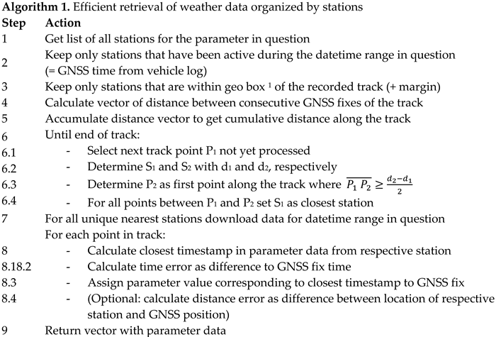 |
| 1 Geo box = min and max latitude and longitude of all considered GNSS fixes. |
For operational use Algorithm 1 will need to be extended with logic for handling invalid station data as well as excessively large time errors – after all, data coming from a station nearby (small distance error) is of limited use if it is simply too old (large time error).
2.5. Efficient Algorithm for Augmenting Vehicle Logs When Data Is Organized in Map Tiles
Data organized in map tiles is interpolated both spatially and temporally in regular intervals: in the case of HERE a new tile is published each 15 minutes and consists of 4096 locations (64 × 64). Algorithm 2 makes use of that fact to improve the speed of data retrieval.
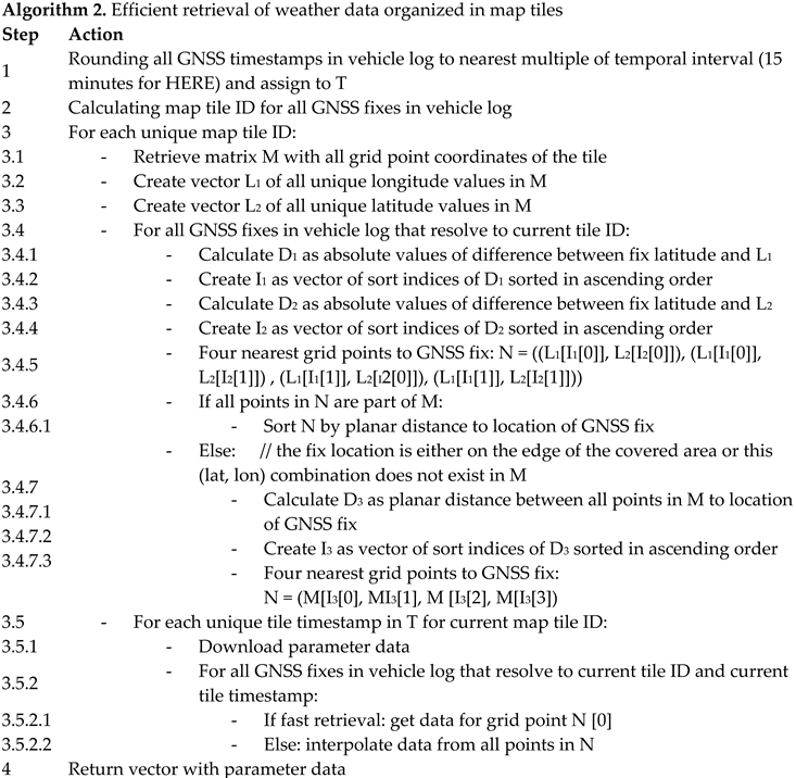 |
For operational use Algorithm 2 will need to be extended with logic for handling missing timestamps and missing map tiles. The fallback solution in step 3.4.7 is much slower but also not executed in the normal case.
3. Results
3.1. Comparison of Air Temperature Measured in Vehicle vs. Measured in Weather Station
The example below shows the importance of knowing the source of the data. The GNSS track of a vehicle driving in the Swedish region of Dalarna from Avesta westwards to Ludvika is used and Figure 7 shows the result of augmenting the vehicle log with air temperature data from SMHI.
The charts below the map in Figure 7 show that the correlation between the air temperature measured on-board the vehicle and the data downloaded from SMHI is not satisfactory. The map reveals the likely reason: apart from the SMHI stations used for the data being rather far away from the road the vehicle travelled on, two of the three stations are placed on ground with an elevation very different from that of to the road. Figure 8 shows the match errors in distance, elevation and time for the SMHI data covering the complete track. The vertical lines with station names do not indicate the position of a station but rather at which point a measurement station starts being used for data retrieval.
The time error plots in Figure 8 varying between -30 and +30 minutes reveals that the measurement interval was 1 hour for the data in question. At a cumulative distance of ca. 46 km at 11:30 UTC the time error jumps from -30 to +30 minutes, indicating that the match algorithm selected the next air temperature value in the measurement sequence as the best fit.
At a cumulative distance of ca. 67 km the time error in Figure 8 suddenly drops from 14 to -18 minutes – but there is no corresponding drop in the plot over time. This simply means that the vehicle didn’t move for 32 minutes, thus no increase in cumulative distance while time advanced as usual. This is also why neither distance error nor elevation error change between 11:45 and 12:20 UTC.
Again, Figure 7 shows an unsatisfactory correlation between the air temperature measured on-board the vehicle and the data downloaded from SMHI. It has been previously mentioned that data from Trafikverket is often more relevant in the context of the research reported on in this paper because the TrV stations are located alongside major roads (though at 6 meter above ground in order to not allow the wind measurements be disturbed by the passing vehicles). In support of this Figure 9 shows a good correlation of the TrV data to the air temperature as measured in the vehicle.
Between 11:45 and 12:20 UTC the correlation gets progressively worse – but the reader is reminded that during that time the vehicle didn’t move. It is uncertain where the air temperature sensor of the vehicle was installed but it is a commonly known phenomenon that measuring ambient temperature in places like a wheel housing or in the side mirror can give rise to such misreading when the vehicle stands still.
The error plots in Figure 10 generally show much lower values than their SMHI counterparts in Figure 8: less distance errors due to denser placement of measurement stations and less time error due to a measurement interval of 30 minutes in TrV’s system “VViS”.
Despite Trafikverket’s measurement stations being only 6 m above ground level the elevation error plots in Figure 10 still show errors up to 140 m. One explanation is that the elevation of the road itself varies, as pictured in Figure 11.
Another explanation for also the matched TrV data showing a certain elevation error is that only the stations in Norberg and Viksberg actually are situated alongside the track of the vehicle. All other stations lie elsewhere, although nearby and alongside other roads in the area. The station in Skeppmora is not that far away from the destination in Ludvika but the area is hilly and thus there is an elevation error of up to 140 m – though this is much less than the SMHI stations’ elevation error of up to 380 m.
3.2. Comparison of Wind Speed and Direction Measured in Weather Stations from SMHI vs. TrV
The previous section underlined the importance of knowing the source of the data. Comparing to data from in-vehicle measurements it has been shown that air temperature from Trafikverket’s stations were a better match than data from SMHI. When it comes to wind data, both speed and direction, there is no such “ground truth” to be found as these parameters are notoriously difficult to assess in a moving vehicle.
Figure 12 shows data from SMHI and TrV matched to the same vehicle log as used previously.
The data do not agree very well. While a certain difference in wind speed can be tolerated the disagreement in wind direction is significant.
Wind is a very local phenomenon where masking by trees or buildings can lead to locally different ground wind speed and direction than what is the case for undisturbed air at a slightly higher altitude. Due to the more relevant location of the TrV stations it can be surmised that whatever is measured by these stations alongside the road is what a vehicle travelling that same road has been subjected to. However, as shown previously in Figure 9 not all stations used are actually placed alongside the vehicle track considered.
Wind data must thus be handled with care. Arguably, aggregating many vehicle logs and corresponding wind speed and direction will still lead to valuable insights on patterns and variations.
3.3. Comparison of Wind Speed and Direction Measured in Weather Stations vs. Interpolated
Both previous two sections stressed that knowing the source of the data is important. It has been stated that interpolating weather data is difficult. Arguably, this is especially critical when it comes to wind data. The differences between the data from SMHI and TrV shown in Figure 12 are striking – even though no interpolation of data has been performed by either agency. In both cases we can thus assume the data to be close to the truth for the location of respective station because they are actual measurement results (in the case of SMHI even quality-reviewed).
In this section interpolated data from the ARCHIVED_WEATHER layer of HERE is matched to the same vehicle log and compared to the station-based data from SMHI and Trafikverket. Since HERE only offers the past 7 days of weather data the timestamps of the original vehicle log are modified to transpose the trip into this time frame. This also enables to compare with high-resolution data from Trafikverket’s RESTful API rather than the medium-resolution data from their long-term VViS database. On the other hand, SMHI data is only available provisionally with quality review still pending (the review process takes 2-3 months).
Figure 13 shows how the data offered by HERE as interpolated values in map tiles is matched to the vehicle track.
Since the data are interpolated there is no way to determine the location of the actual measurement stations and the timestamps of the actual measurements. Thus it is meaningless to calculate the distance, elevation and time errors.
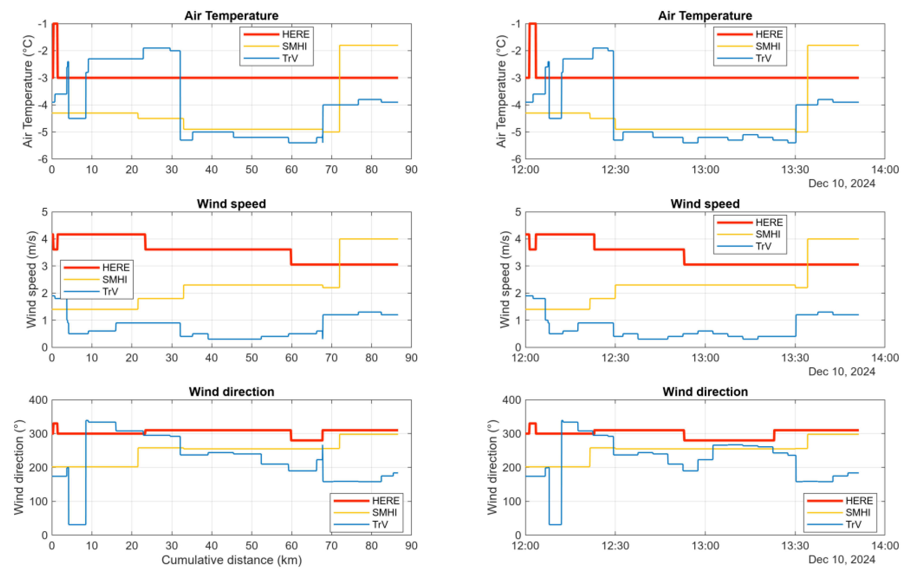
Figure 14 shows a comparison of the air temperature, wind speed and wind direction data from HERE, SMHI (not quality-reviewed) and TrV (high-resolution data from their RESTful API) matched to the same vehicle log as used previously, but shifted in time to begin at 12:00 UTC on 10 December 2024 (data was accessed on 13 December 2024).
It is apparent that the data from HERE do not agree very well to the data from either SMHI or Trafikverket. Lacking information on the data sources as well as how interpolation is performed, the conclusion is that non-interpolated data from identifiable measurement stations, placed on relevant locations is to be preferred.
4. Discussion
The results of the work presented in this paper are to be understood as enablers for future research. Various sources for data from weather observations and the way data is organized and made accessible have been discussed in principle and specifically. Two algorithms have been presented for efficiently extraction of such weather data and augmentation of vehicle logs in order to perform studies on energy efficiency. These vehicle logs can of course be recorded in actual vehicle operation or simulated.
Using these algorithms it has been further shown how a critical review of the results can be aided by examining the distance, elevation and time errors. The examples given in this paper support the conclusion that it is preferred to retrieve data from sources where it is organized by identifiable weather stations, rather than being interpolated and organized in map tiles. Furthermore, the conclusion is that it is preferred to utilize data sources where the weather stations are placed in the area of vehicle operation, i.e., alongside the road network.
5. Conclusions
With the results presented in this paper it is now possible to study a massive amount of vehicle logs, recorded and simulated, and put them into their meteorological context. This will enable new insights regarding energy losses due to environmental interaction, both in size and distribution.
Funding
This research was supported by funding from VINNOVA for the project “Solar cells on trucks for environmental friendly transport” within the venture “Challenge-driven innovation - Phase 2 Collaboration” and the Swedish Energy Agency for the project “Customer Oriented Operations Research for Electrification (CONDORE)” within the framework of the program FFI, Fordonsstrategisk Forskning och Innovation.
Conflicts of Interest
The author declares no conflicts of interest. The funders had no role in the design of the study; in the collection, analyses, or interpretation of data; in the writing of the manuscript; or in the decision to publish the results.
References
- Sandberg, T. Heavy Truck Modeling for Fuel Consumption: Simulations and Measurements. Licentiate Thesis, Linköpings Universitet, Linköping, Sweden, 2001. [Google Scholar]
- Beulshausen, J.; Pischinger, S; Nijs, M. Drivetrain Energy Distribution and Losses from Fuel to Wheel. SAE Int. J. Passeng. Cars-Mech. Syst. 2013, 6(3), 1528–1537. [CrossRef]
- Filla, R. Operator and Machine Models for Dynamic Simulation of Construction Machinery. Licentiate Thesis, Linköpings Universitet, Linköping, Sweden, 2005. [Google Scholar]
- Hyttinen, J. Modelling and experimental testing of truck tyre rolling resistance. Doctoral Thesis, KTH Royal Institute of Technology, Stockholm, Sweden, 2023. [Google Scholar]
- Askerdal, M. On motion resistance estimation and modeling for heterogeneous road vehicles. Licentiate Thesis, Chalmers, Göteborg, Sweden, 2023. [Google Scholar]
- Dalessio, L.; Bradley, D.; Chang, C.; Gargoloff, J. et al. Accurate Fuel Economy Prediction via a Realistic Wind Averaged Drag Coefficient. SAE Int. J. Passeng. Cars-Mech. Syst. 2017, 10(1), 265–277. [CrossRef]
- Kaminski, M.; Borton, Z. Development, Application, and Implementation of Passenger Vehicle Wind Averaged Drag for Vehicle Development. SAE Technical Paper 2024-01-2532, 2024. 2532. [CrossRef]
- Barry, N. A New Method for Analysing the Effect of Environmental Wind on Real World Aerodynamic Performance in Cycling. Proceedings 2018, 2, 211. [Google Scholar] [CrossRef]
- Peng, Y.; Jilang, Y; Lu, J.; Zou, Y. Examining the effect of adverse weather on road transportation using weather and traffic sensors. PLoS ONE 2018, 13(10), e0205409. PLoS ONE 2018, 13(10), e0205409. [CrossRef]
- Almkvist, E.; David, M.; Pedersen, J.; Lewis-Lück, R. et al. Enhancing Autonomous Vehicle Safety in Cold Climates by Using a Road Weather Model: Safely Avoiding Unnecessary Operational Design Domain Exits. SAE Int. J. Passeng. Veh. Syst. 2024, 17(1), 49–63, 2024. [CrossRef]
- Neumann, O.; Turowski, M.; Mikut, R.; Hagenmeyer, V.; et al. Using weather data in energy time series forecasting: the benefit of input data transformations. Energy Inform 2023, 6, 44. [Google Scholar] [CrossRef]
- SMHI’s Open Data. Available online: https://www.smhi.se/en/services/open-data/search-smhi-s-open-data (accessed on 5 December 2024).
- Trafikverket’s Data Exchange Portal. Available online: https://data.trafikverket.se/home (accessed on 5 December 2024).
- MET Norway’s FROST API. Available online: https://frost.met.no/index.html (accessed on 5 December 2024).
- Deutscher Wetterdienst CDC-Portal. Available online: https://www.dwd.de/EN/ourservices/cdc_portal/cdc_portal.html (accessed on 5 December 2024).
- Finnish Meteorological Institute’s Open Data. Available online: https://en.ilmatieteenlaitos.fi/open-data (accessed on 5 December 2024).
- RODEO project. Available online: https://rodeo-project.eu (accessed on 5 December 2024).
- HERE Map Attributes API - Developer Guide: Maps & layers. Available online: https://www.here.com/docs/bundle/map-attributes-api-developer-guide/page/topics/here-map-content.html (accessed on 5 December 2024).
- REST API Tutorial. Available online: https://restfulapi.net (accessed on 5 December 2024).
- Bright Sky: JSON API for DWD open weather data. Available online: https://brightsky.dev (accessed on 5 December 2024).
Figure 1.
Main principles of data organization and access.
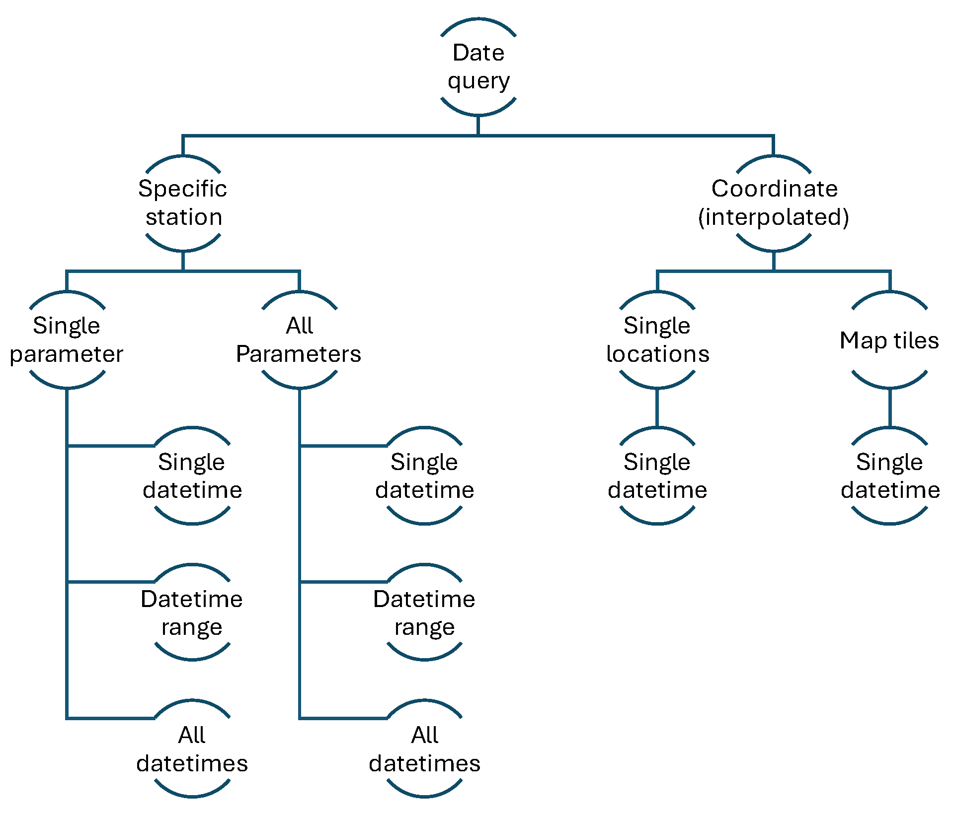
Figure 2.
Example of data organized in map tiles.
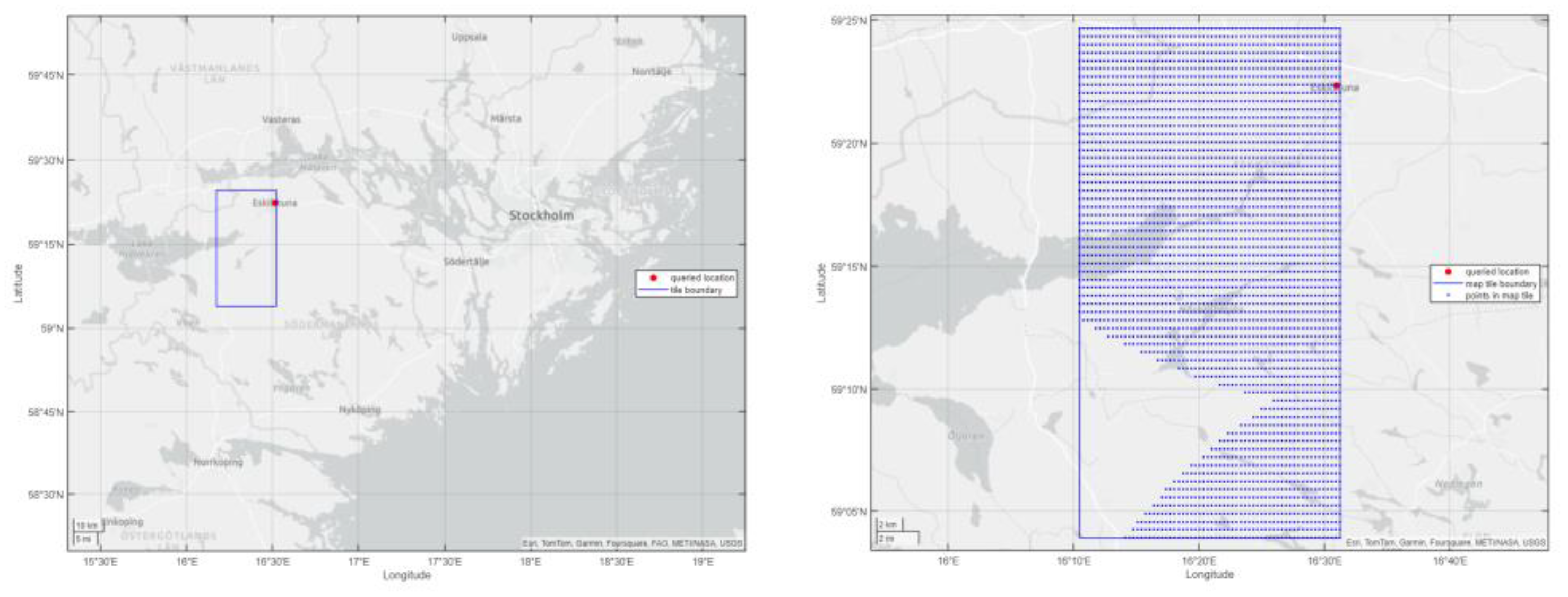
Figure 3.
Most critical case: straight track.
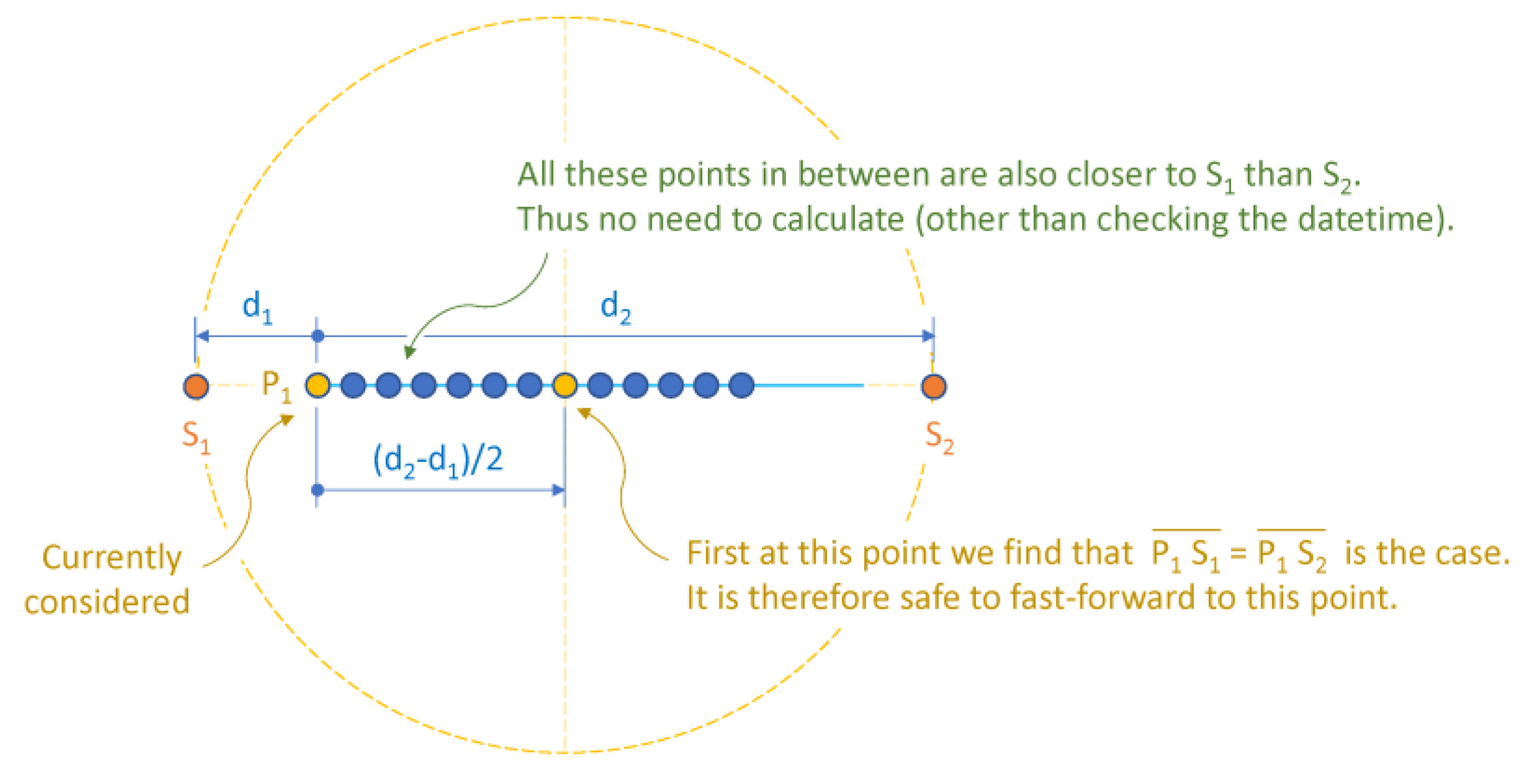
Figure 4.
Less critical case: curved track.
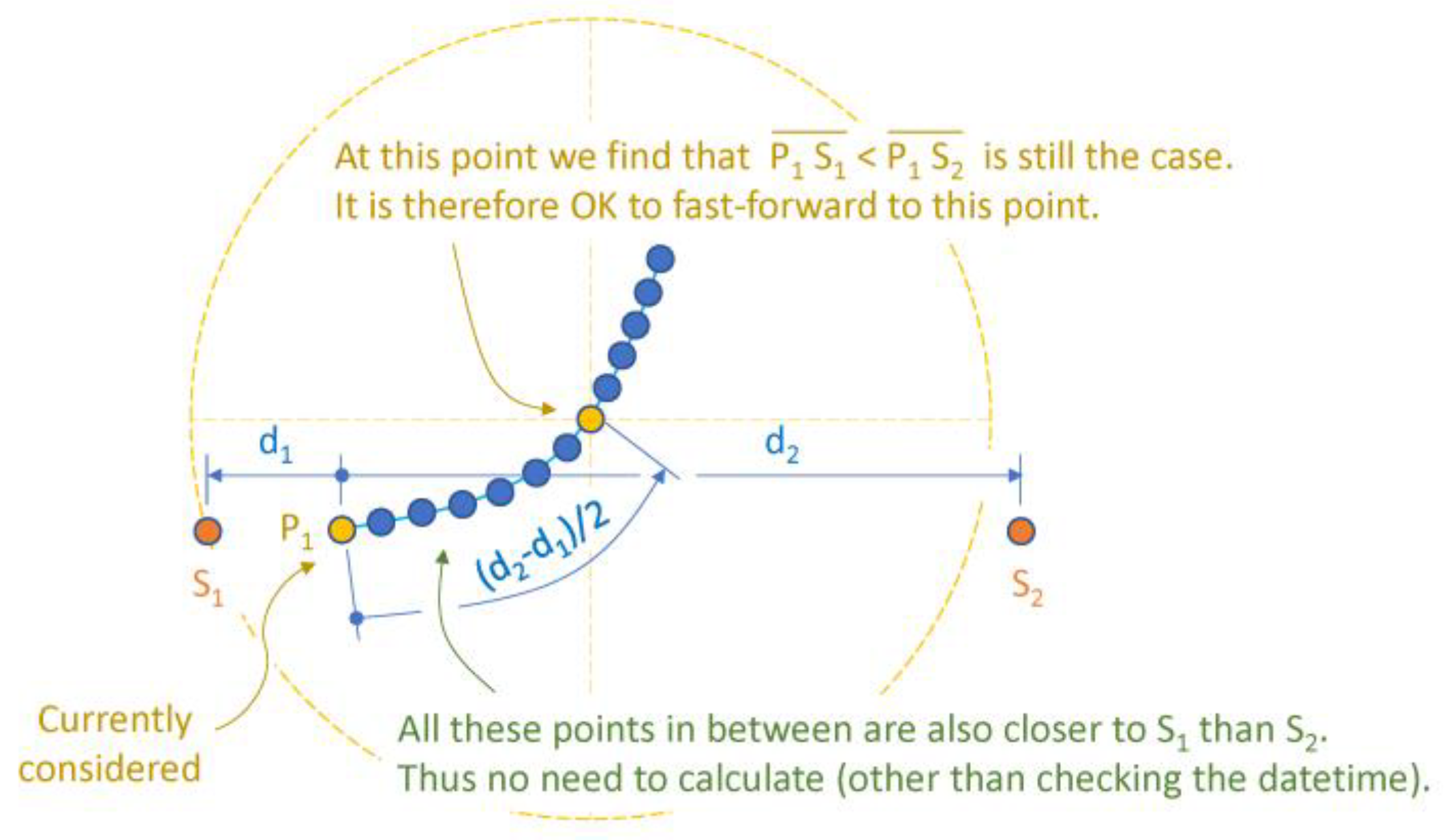
Figure 5.
Considering third-nearest station.
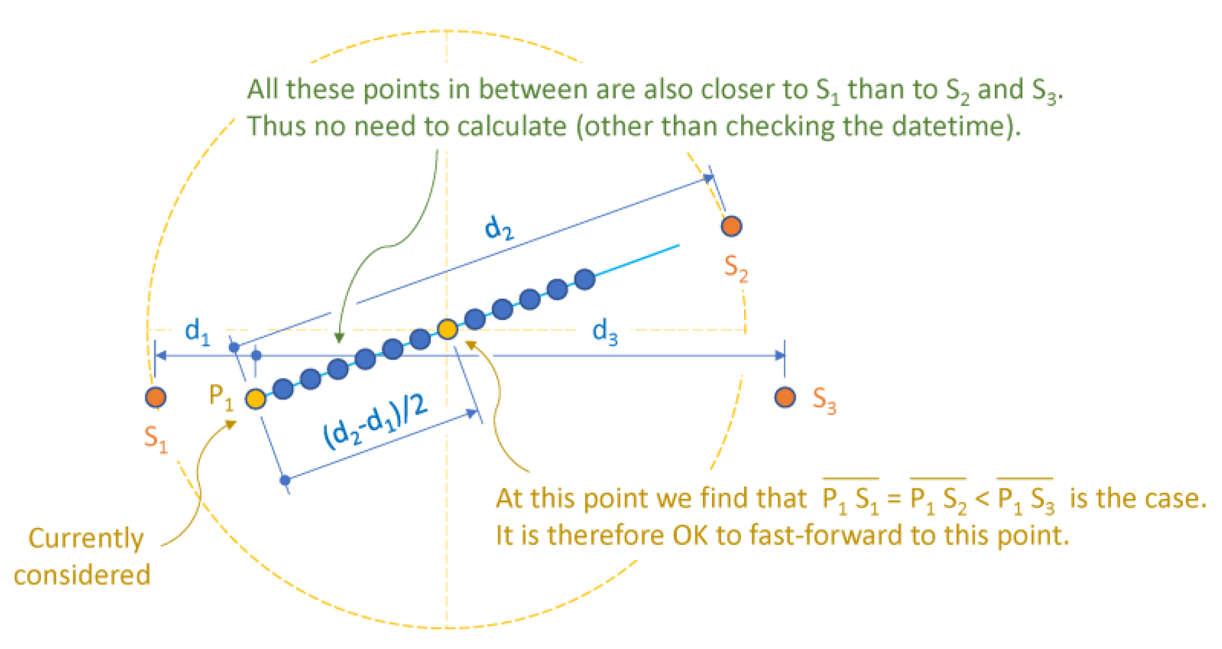
Figure 6.
Considering third-nearest station: most critical case.
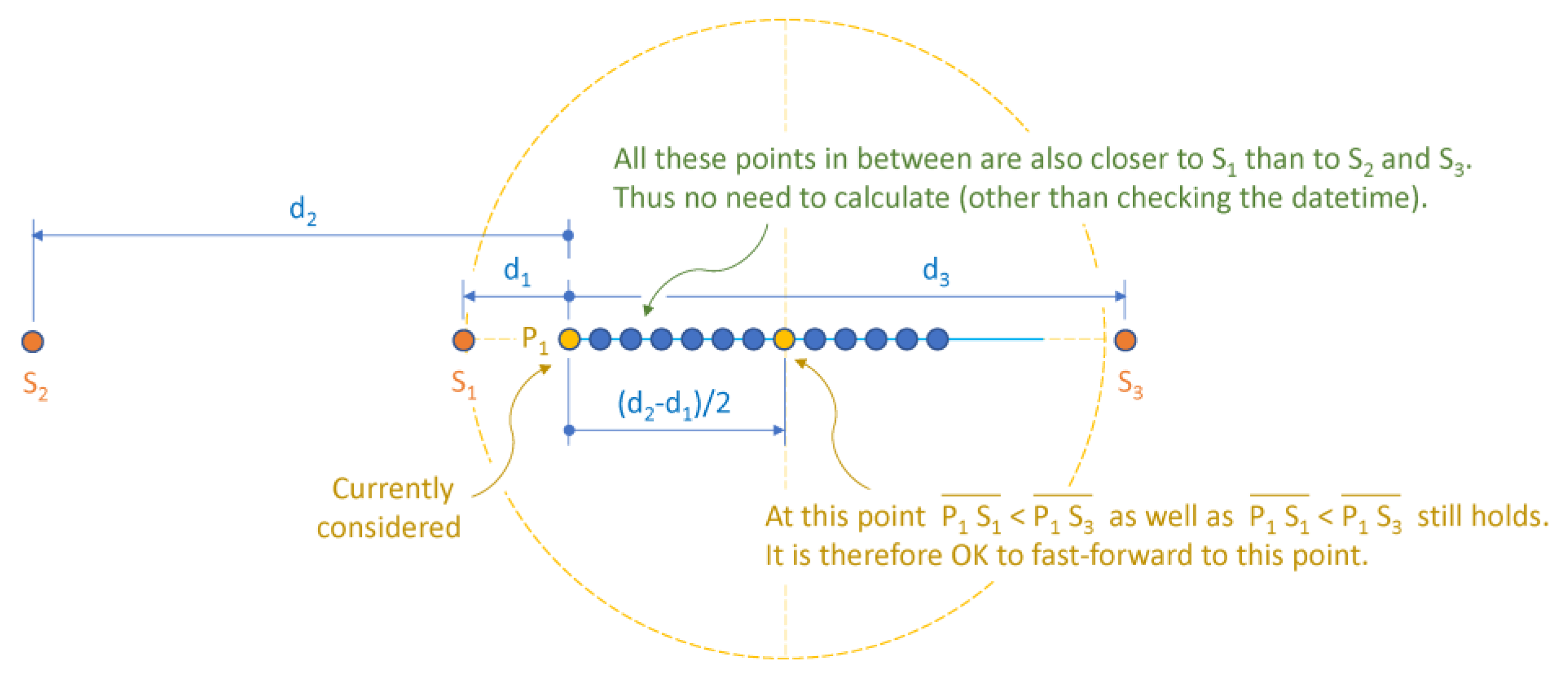
Figure 7.
Air temperature data from SMHI matched to a vehicle log.
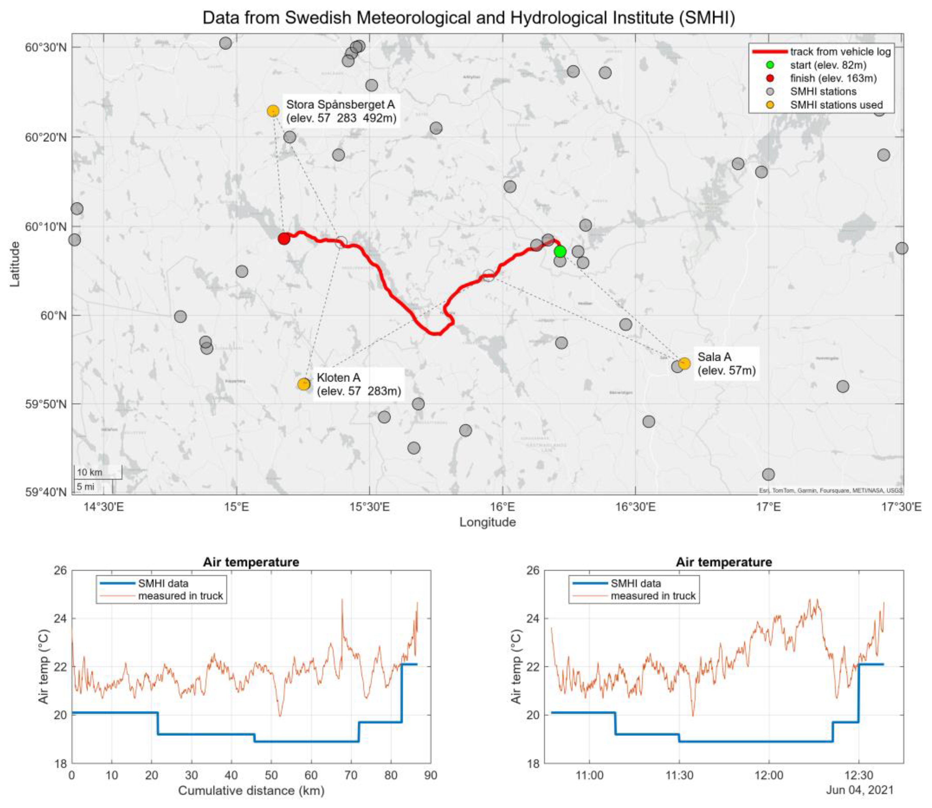
Figure 8.
Distance, elevation and time error for the SMHI data in Figure 7.
Figure 8.
Distance, elevation and time error for the SMHI data in Figure 7.
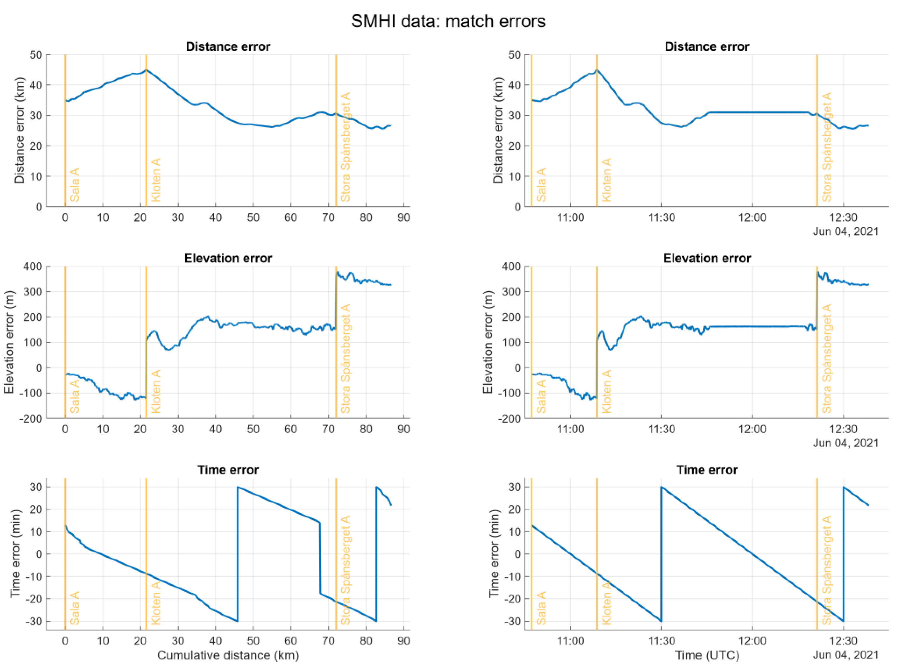
Figure 9.
Air temperature data from Trafikverket matched to the same vehicle log.
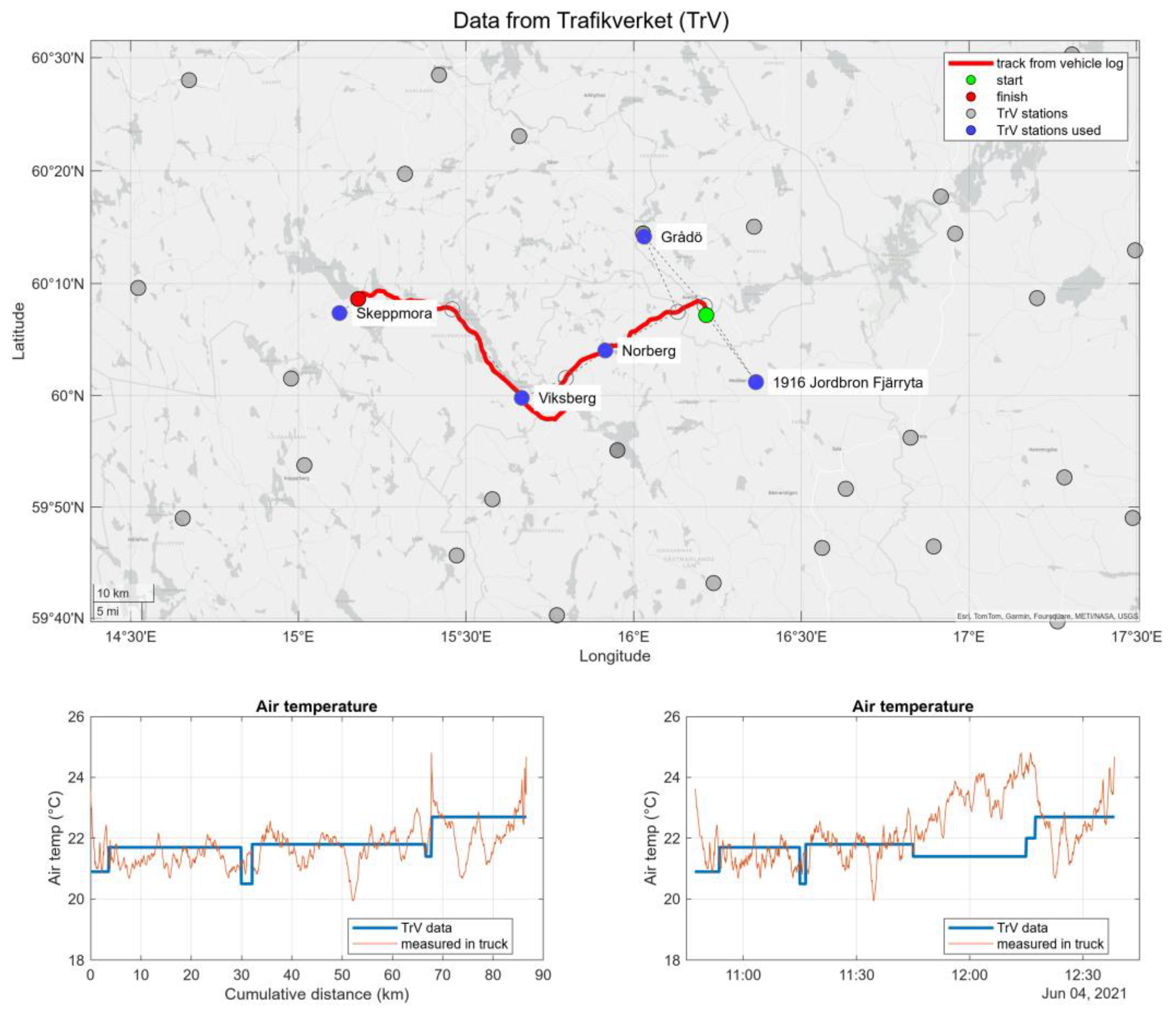
Figure 10.
Distance, elevation and time error for the TrV data (VViS) in Figure 9.
Figure 10.
Distance, elevation and time error for the TrV data (VViS) in Figure 9.
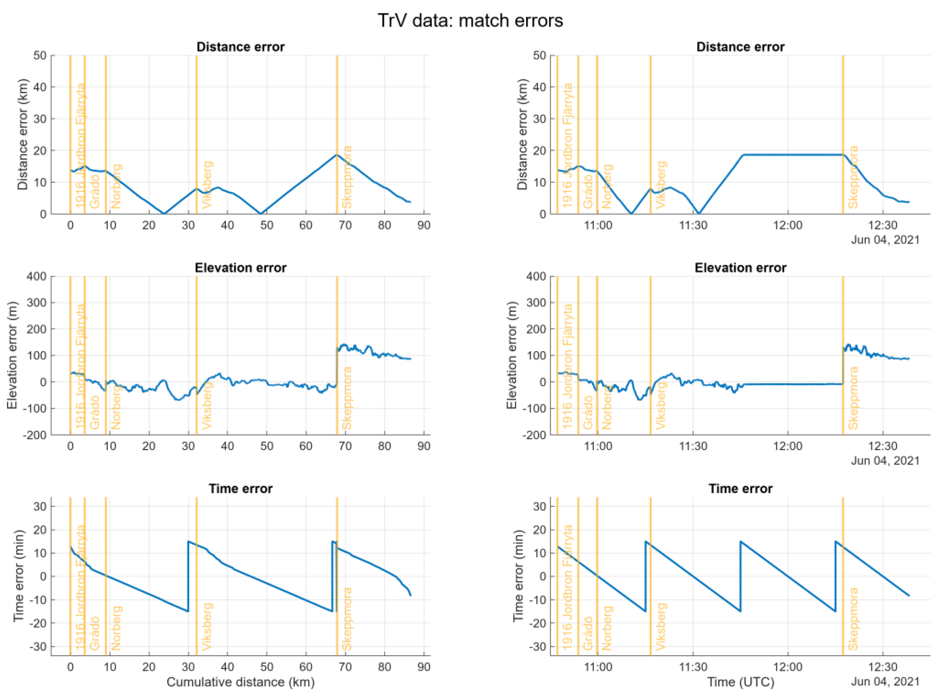
Figure 11.
Elevation of the road and the measurement stations used.
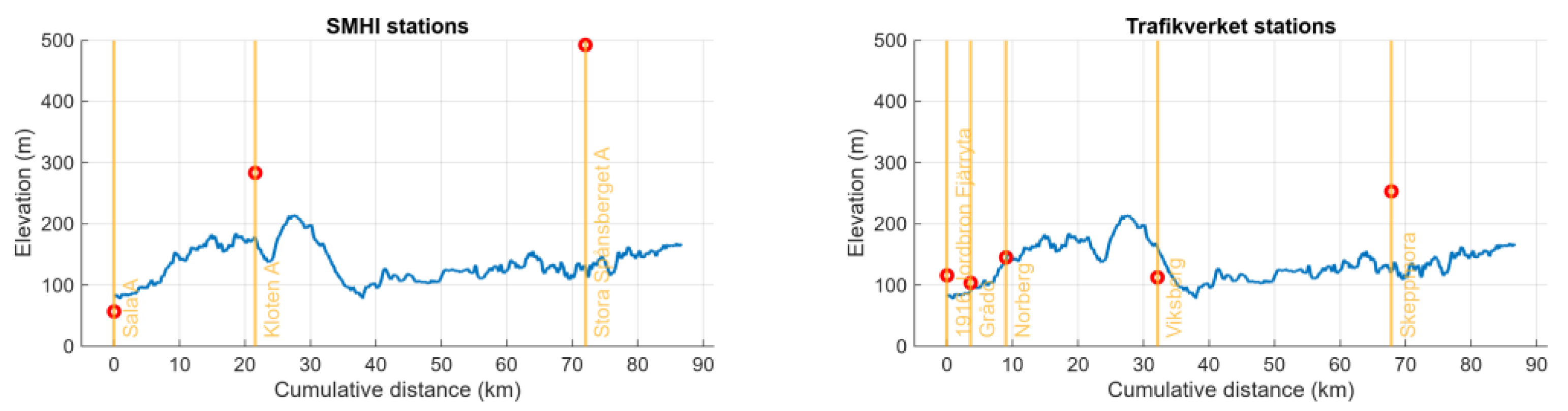
Figure 12.
Wind speed and wind direction fetched from SMHI and TrV (VViS).
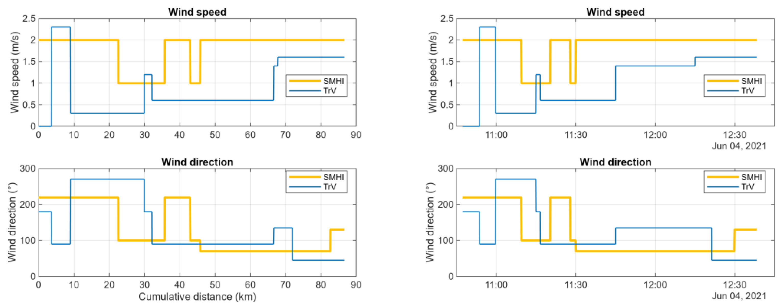
Figure 13.
HERE grid points used to match the vehicle track.
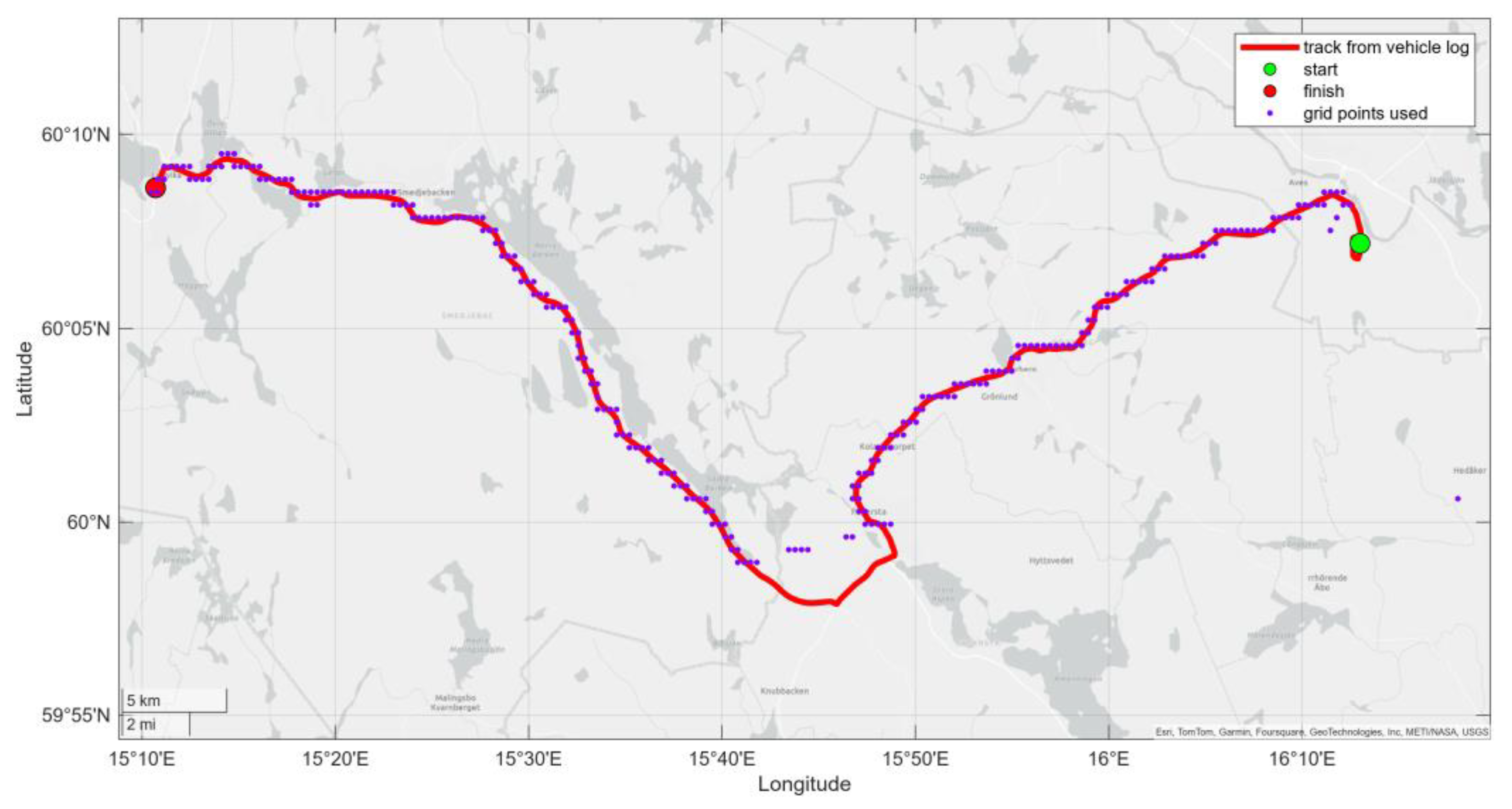
Figure 14.
Wind speed and wind direction fetched from HERE, SMHI and TrV (REST).
Disclaimer/Publisher’s Note: The statements, opinions and data contained in all publications are solely those of the individual author(s) and contributor(s) and not of MDPI and/or the editor(s). MDPI and/or the editor(s) disclaim responsibility for any injury to people or property resulting from any ideas, methods, instructions or products referred to in the content. |
© 2024 by the authors. Licensee MDPI, Basel, Switzerland. This article is an open access article distributed under the terms and conditions of the Creative Commons Attribution (CC BY) license (http://creativecommons.org/licenses/by/4.0/).
Copyright: This open access article is published under a Creative Commons CC BY 4.0 license, which permit the free download, distribution, and reuse, provided that the author and preprint are cited in any reuse.


