Submitted:
13 December 2024
Posted:
13 December 2024
You are already at the latest version
Abstract
To address the interdependence of local time-frequency information in audio scene recognition, a segment-based time-frequency feature fusion method based on Cross-Attention is proposed. Since audio scene recognition is highly sensitive to individual sound events within a scene, the input features are segmented into multiple segments along the time dimension to obtain local features, allowing the subsequent attention mechanism to focus on the time slices of key sound events. Furthermore, to leverage the advantages of both Convolutional Neural Networks (CNNs) and Recurrent Neural Networks (RNNs), which are mainstream structures in audio scene recognition tasks, this paper employs a parallel structure to separately obtain the time-frequency features output by CNNs and RNNs, and then fuses the two sets of features using Cross-Attention. Experiments on the TUT2018, TAU2019, and TAU2020 datasets demonstrate that the performance of this algorithm improves the official baseline results by 17.78%, 15.95%, and 20.13%, respectively.
Keywords:
audio scene recognition
; feature fusion
; cross-attention
; convolutional neural networks
; recurrent neural networks
1. Introduction
Acoustic scene classification (ASC) and sound event detection are important techniques for the computational analysis of natural acoustic scenes. These tasks typically serve as the front end of audio processing and include the recognition of indoor scenes, outdoor scenes, public spaces, and office environments. They also encompass a variety of application scenarios, such as wearable devices, healthcare equipment, monitoring devices, autonomous driving, and other devices that require environmental awareness [1].
Early research on audio scene classification typically focused on perceptual features of the human auditory system, combined with classic machine learning algorithms such as Hidden Markov Model (HMM) and Gaussian Mixture Model (GMM). For example, Clarkson et al [2]. calculated Mel-scale filter bank coefficients for ASC. Couvreur et al.[3] used Linear Predictive Cepstral Coding (LPCC) features and discrete HMMs to identify five types of sound events. Maleh et al.[4] classified five types of environmental noise using line spectrum features and Gaussian classifiers. Eronen et al.[5] proposed an ASC system based on Mel-Frequency Cepstral Coefficients (MFCC), classifying different acoustic scenes using GMM/HMM, and in subsequent work, further classified 18 different acoustic scenes based on a richer set of acoustic features, achieving an overall accuracy of 58%. In addition to acoustic features, Heittola et al.[6] also performed scene classification using event histograms.
With the development of deep learning methods, the performance of ASC systems has significantly improved. For example, Valenti et al.[7] converted audio files into log-Mel spectrograms as input to train CNN models. Xu et al.[8] proposed an improved deep neural networks (DNNs) classification method, achieving performance improvements of 10.8% and 22.9% compared to classical DNNs structures and GMMs. Additionally, extensions to the CNN architecture have been shown to enhance feature learning performance. For instance, Basbug et al.[9] employed a spatial pyramid pooling strategy to pool and combine feature maps at different spatial resolutions, achieving a classification accuracy of 59.5% on the DCASE dataset. Zhang et al.[10] proposed an end-to-end CNN for ASC systems. Madhu et al.[11] introduced the quaternion residual convolutional network RQNet, further improving the performance of ASC systems. Temporal networks can also be applied in ASC research. For example, Zöhrer et al.[12] used Gated recirculation unit (GRU) and linear discriminant analysis to classify different audio scenes. Li et al.[13] utilized a Bidirectional Long Short-Term Memory network (Bi-LSTM) as a classifier to map MFCC features. Vij et al [14] employed LSTM to learn Log-Mel features.
The above researches on algorithms indicate that Convolutional Neural Networks (CNNs) and Recurrent Neural Networks (RNNs) are beneficial for enhancing the performance of ASC. However, these algorithms are typically used independently as either CNN or RNN networks. To combine the advantages of both, some studies have connected CNNs and RNNs for ASC tasks [15]. In contrast, this paper adopts a parallel approach, first extracting embedded features from both CNN and RNN separately. Then, it utilizes cross-attention to fuse the embedded features, using the temporal features output by the RNN as Query to provide a time dimension weighting for the time-frequency features extracted by the CNN. Finally, a classifier built with a fully connected neural network is used to obtain the audio scene categories. On the TUT2018 dataset, this algorithm outperformed the concatenated RNN-CNN algorithm [15] by 3.88%.
2. Network Structure
The proposed parallel CNN-RNN model based on Cross-attention is illustrated in the Figure 1. The model uses Log-Mel features as input; However, directly using these features may struggle to capture the correlations of different sound events specific to certain scenes, which can limit the performance of the ASC system. To address this, the study employs time-domain segmented Log-Mel features as inputs for both CNN and RNN, denoted as and , respectively, the input segment-level features denoted as ,The two modules help the ASC system obtain high-level segment features based on time-frequency and temporal information, which can be represented as:
Where N is the number of segments in the time domain of the spectrogram, and C is the dimension of the outputs from different modules, meaning that the number of hidden units in the RNN is set to be consistent with the output dimension of the CNN. The CNN network is composed of residual convolutional blocks, while the RNN consists of 2 layers of GRU. Then, the features are fused through Cross-attention, where the features from the RNN serve as the Query in the attention mechanism. Based on the attention scores, the fused features are weighted and summed along the time dimension. Finally, the classification results for ASC are obtained through a classifier constructed with fully connected neural networks.
3. Algorithm
3.1. Segment-Level Features
The ASC system typically needs to consider the large number of complex local environments in acoustic data. However, a segment of scene audio may contain multiple sound events, and audio recorded in different scenes may have similar sound events. For example, the rumble of a tram may occur both inside the carriage and at the station, music may be present in both a cafe and a restaurant, and birdsong may be heard in both a park and on the street. In most cases, audio scenes usually include sound events, noise, or echoes, as well as their combinations. There may even be audio segments that do not contain any obvious events, such as long periods of silence or quietness. Generally, people can perceive the scene of a park through the sounds of birds and streams, but if there is no event information in the park, the ASC system will struggle to distinguish whether it is a park or another outdoor scene. Therefore, audio segments may contain specific sounds that represent a scene or may only include common sounds that can occur in multiple scenes. If the audio contains sounds specific to a certain scene, the scene can be identified more accurately within the same category; However, if not, it becomes difficult to make distinctions among these sounds.
In a long-duration recorded audio dataset, there may be multiple sound events. As shown in Figure 2, each event information is sufficient to express multiple corresponding environments, and there can be common features between different scenes. For example, both parks and squares may contain a lot of quiet segments, and the rumble of cars can be heard in both traffic streets and squares. Therefore, simply identifying a single event may make it difficult to accurately determine the environment. Additionally, in some real recorded scene audio, relevant information may have a short duration, such as the honking of cars at a bus station or the rumble of planes taking off at an airport. Thus, the scene information contained in a segment of audio may be limited and dispersed, meaning that there may be a lot of irrelevant information in the recorded audio. Consequently, audio data based on combinations of multiple acoustic events makes it challenging for existing ASC systems to capture specific scene information, especially for temporal models, where long periods of non-semantic environmental information may hinder their ability to effectively focus on specific event information. In light of this, to assist the ASC system in acquiring scene information, the input of the model designed in this paper consists of segment-level spectrogram features segmented along the time axis. Here, the original spectrogram can be represented as , and the temporally correlated segment-level features can be represented as , , where T and F represent the time scale and frequency scale of the spectrogram, respectively. In the experimental phase, further research will be conducted on the impact of the number of segments N on system performance.
3.2. Residual Convolution
The Residual Neural Network (ResNet) was proposed by Kaiming He and others in 2015 [16]. Its main contribution lies in identifying and addressing the "degradation phenomenon" that exists in deep neural networks. The degradation phenomenon refers to the issue where, as the depth of the network increases, the training error also increases, leading to a decline in performance. To solve this problem, He and his team introduced the concept of "shortcut connections," which allow for skip connections in the network, enabling information to be transmitted more directly between layers. This structure greatly alleviates the training difficulties of deep neural networks, allowing for the construction of deeper networks while maintaining good performance. The success of ResNet has laid an important foundation for subsequent research in deep learning.
The residual structure used in this paper is shown in the blue dashed box in Figure 1. The residual block consists of two 3x3 convolutional layers with the same number of output channels, each followed by a batch normalization layer and a ReLU activation function. Through a cross-layer data pathway, the input is added directly before the final ReLU activation function, skipping the two convolution operations within the residual block. This design requires that the outputs of the two convolutional layers have the same shape as the input, ensuring that the output of the second convolutional layer matches the original input shape for addition. When the number of channels differs, an additional 1x1 convolutional layer is needed to transform the input into the required shape before performing the addition. The principle is that the 1x1 convolutional layer does not alter anything in the spatial dimension, and it primarily changes the channel dimension.
3.3. Gated Recurrent Unit
The Gated Recurrent Unit (GRU) proposed by Cho was originally applied in the field of machine translation [17]. Its core idea is that feature vectors at different distances in the hidden layer have varying impacts on the current hidden state, with the influence diminishing as the distance increases. The GRU introduces a gating mechanism to control the flow of information, effectively capturing long-term dependencies. Its main components include the reset gate and the update gate, which allow the model to flexibly choose which information to retain and which to update, resulting in excellent performance when handling sequential data.The specific computation methods can be found in Equations (3) —(6), and a structural diagram of the GRU is illustrated in the chocolate-colored dashed box in Figure 1.
Where ⊙ represents Hadamard product. is the update gate, which controls the amount of historical information retained at the current time step, thereby helping the RNN remember long-term dependencies. is the reset gate. when its value is 0, it indicates that it is turned off. In this case, the candidate hidden layer output is determined solely by the current input and is independent of historical outputs. This allows the hidden state to effectively discard irrelevant information from the historical data, resulting in a more robust compressed representation.
3.4. Cross-Attention
The implementation of cross-attention is derived from the self-attention mechanism [18], but it considers data from different sources when processing inputs. In the self-attention mechanism, the Query, Key, and Value typically come from the same data source. In this paper, the output features of the GRU are used as the Query, while the output features of the CNN are used as the Key and Value. The calculation method is as follows:
The Q , K , and V are obtained through projection transformations by and , where are parameters to be learned by the network and have the same dimension. In Equation (10), the attention scores are obtained using the softmax function, where N corresponds to the number of time segments. To prevent the inner product from becoming too large when calculating the of each row vector of matrices Q and K , a scaling factor is applied. Finally, the attention mechanism scores are used to perform a weighted sum of the values V along the time dimension.
4. Experiments and Discussion
4.1. Datasets
To validate the effectiveness of the proposed algorithm, experiments were conducted on three databases provided by the Detection and Classification of Acoustic Scenes and Events Challenge [19].
TUT 2018 is a publicly available dataset recording ten different acoustic scenes from six European cities, specifically: airport, indoor shopping mall, subway station, pedestrian street, public square, traffic street, tram, bus, subway, and urban park. Each acoustic scene in TUT 2018 consists of 864 segments, totaling 8,640 audio clips. The training set contains 6,122 samples, while the test set includes 2,518 samples.
TAU 2019 is an extended version of the TUT 2018 dataset, expanding from six European cities to twelve. However, the development dataset includes only ten of these cities and contains the same ten acoustic scenes as the TUT 2018 dataset. In the officially designated training and test sets, the training set consists solely of audio data from nine cities to evaluate the system’s generalization capabilities. This dataset comprises 40 hours of recorded data across 14,400 audio files, with 9,185 files allocated to the training set and the remaining files used as the test set.
TAU 2020 builds upon the TAU 2019 dataset, further expanding the acoustic scene classification by using four different devices to simultaneously record data. This includes three portable devices, such as smartphones and cameras, as well as synthetic data created from audio recorded by multiple devices. TAU 2020 contains data from ten acoustic scenes across twelve European cities, recorded at a sampling rate of 44.1 kHz, with a total duration of 64 hours. The dataset includes 13,965 samples for training and 2,970 samples for testing.
4.2. The Impact of Time Segmentation
To test the impact of segment-level feature model inputs at different time scales on system performance, the maximum number of segments N for the Log-Mel features based on the time domain is set to 10, indicating that global features are used as input. The models tested include:
- CNN+SA: An independent CNN model followed by self-attention;
- GRU+SA: An independent GRU model followed by self-attention;
- CNN-GRU+CA: A proposed parallel CNN and GRU model followed by cross-attention.
When N = 1 , the attention mechanism uses frame-level features as input, since Log-Mel features require audio to be segmented into frames for feature extraction. By comparing these models, the impact of different time-scale feature inputs on system performance can be evaluated, as shown in Figure 3, Figure 4 and Figure 5.
For the independent CNN network, the trend observed across the three databases indicates that as the number of segments increases, the recognition performance initially improves, but declines when the number of segments becomes too high. This is because each sound scene typically consists of only a few types of sound events; for example, in a park scene, there may only be bird chirping and silence as sound events. When the number of segments is excessive, the subsequent attention scores become dispersed, making it difficult to focus on the key sound events. However, the optimal number of segments is uncertain. Experiments conducted on the TUT2018, TAU2019, and TAU2020 datasets show that the best performance was achieved with segment counts of 6, 4, and 5, yielding recognition rates of 73.47%, 75.71%, and 68.67%, respectively.
For the independent GRU network, as the number of segments increases, the performance of the GRU shows some improvement and eventually stabilizes. This means that an excessive number of segments does not lead to further performance enhancement, but it does not cause a significant decline like in CNNs. This is because GRUs have memory capabilities, giving them an advantage in processing sequential data. On the TUT2018, TAU2019, and TAU2020 datasets, the best performances achieved by the GRU were 72.7%, 73.46%, and 65.46%, respectively. Although the best performance of the GRU is not as high as that of the CNN, this is because CNNs balance both temporal and frequency domain computations more effectively. Therefore, in the research of ASC, there is relatively more focus on CNNs.
The parallel CNN-GRU network, utilizing cross-attention for feature fusion, demonstrates significantly better performance compared to independent CNN and GRU models. On the TUT2018, TAU2019, and TAU2020 datasets, the best performances achieved are 77.48%, 78.45%, and 71.73%, respectively. This approach combines the CNN’s ability to process time-frequency information with the GRU’s memory capability for sequential information.In the temporal dimension, the sequential features provided by the GRU are used to apply attention weighting to the time-frequency features extracted by the CNN. This enhances the characteristics of key sound events in the audio scene, thereby improving the overall system performance.
4.3. Feature Fusion
To verify the effectiveness of feature fusion based on the cross-attention algorithm, this study compared it with the following models: the outputs of the parallel CNN-GRU structure were concatenated along the temporal dimension, and then self-attention was applied to the concatenated features for fusion, referred to as CNN-GRU+CO+SA. In terms of model structure, the CNN and GRU models were concatenated, and self-attention was applied based on the order of concatenation, referred to as CNN+GRU+SA and GRU+CNN+SA, respectively. The results are shown in Table 1.
Compared to the concatenated models, the two parallel CNN-GRU structures demonstrated better performance because they could better leverage the advantages of both CNNs and RNNs. In contrast, the concatenated structure increased the depth of the network, making training more challenging and potentially causing the advantages of the preceding CNN/GRU to be lost in the subsequent GRU/CNN structure. Additionally, while CNN-GRU+CO+SA, which directly concatenates the outputs of CNN and GRU, achieved better performance than the serial structure, the differences in feature spaces between the CNN and GRU outputs reduced the expressive power of the fused features, resulting in performance that was not as good as CNN-GRU+CA.
In addition, we compared our results with other studies in the literature. The DCASE refers to the baseline results provided by the Detection and Classification of Acoustic Scenes and Events Challenge. All these studies utilized CNN structural units. Under the same dataset, the performance of our proposed algorithm surpassed that of the aforementioned studies. On the TUT2018, TAU2019, and TAU2020 datasets, our method improved the official baseline results by 17.78%, 15.95%, and 20.13%, respectively.
5. Conclusions
In the task of ASC, both CNN and RNN structures have their advantages. To combine the strengths of both, we proposed a method that uses Cross-attention to fuse the output features of parallel CNN-RNN structures, allowing them to form complementary information. In this paper, the output features of the GRU are used as the Query in the attention mechanism to calculate attention scores for the time-frequency features from the CNN output, applying weighting along the temporal dimension. Since sound scene recognition is often highly correlated with specific sound events within the scene, we sliced the input features along the temporal dimension, enabling the subsequent attention mechanism to focus the weighting scores on these representative sound event slices. Experimental results indicate that the proposed CNN-GRU+CA model shows improved performance compared to existing algorithms.
Author Contributions
Conceptualization, Rong Huang and Yue Xie; methodology, Rong Huang; validation, Pengxu Jiang and Yue Xie; formal analysis, Rong Huang and Yue Xie; investigation, Pengxu Jiang; writing—original draft preparation, Rong Huang;
Data Availability Statement
Datasets TUT2018, TAU2019 and TAU2020 are provided by the Detection and Classification of Acoustic Scenes and Events Challenge
Conflicts of Interest
The authors declare no conflicts of interest.
References
- Abeßer, J. , A Review of Deep Learning Based Methods for Acoustic Scene Classification. Applied Sciences, 2020. 10.
- B. Clarkson, N. Sawhney, and A. Pentland, “Auditory context awareness via wearable computing,” in Proc. 1998 Workshop Perceptual User Interfaces (PUI98), 1998.
- Couvreur C, Gaunard P, Cg. M,et al.Automatic classification of environmental noise events by hidden Markov models.Applied acoustics, 1998(3):54.
- K. El-Maleh, A. Samouelian and P. Kabal, "Frame level noise classification in mobile environments," 1999 IEEE International Conference on Acoustics, Speech, and Signal Processing. ICASSP99, Phoenix, AZ, USA, 1999, pp. 237-240 vol. 1.
- A. Eronen et al., "Audio-based context awareness - acoustic modeling and perceptual evaluation," 2003 IEEE International Conference on Acoustics, Speech, and Signal Processing, 2003. Proceedings. (ICASSP ’03)., Hong Kong, China, 2003, pp. V-529. [CrossRef]
- T. Heittola, A. Mesaros, A. J. Eronen, and T. Virtanen, “Audio context recognition using audio event histogram,” in Proc. European Signal Processing Conf. (EUSIPCO), 2010.
- M. Valenti, A. Diment, G. Parascandolo, S. Squartini, and T. Virtanen,“DCASE 2016 acoustic scene classification using convolutional neural networks,” DCASE2016 Challenge, Tech. Rep., September 2016.
- Y. Xu, Q. Huang, W. Wang, and M. D. Plumbley, “Hierarchical learning for DNN-based acoustic scene classification,” DCASE2016 Challenge, Tech. Rep., September 2016.
- A. M. Basbug and M. Sert, "Acoustic Scene Classification Using Spatial Pyramid Pooling with Convolutional Neural Networks," 2019 IEEE 13th International Conference on Semantic Computing (ICSC), Newport Beach, CA, USA, 2019, pp. 128-131.
- L. Zhang, J. Han and Z. Shi, "Learning Temporal Relations from Semantic Neighbors for Acoustic Scene Classification," in IEEE Signal Processing Letters, vol. 27, pp. 950-954, 2020. [CrossRef]
- A. Madhu and S. K, "RQNet: Residual Quaternion CNN for Performance Enhancement in Low Complexity and Device Robust Acoustic Scene Classification," in IEEE Transactions on Multimedia.
- M. Zöhrer and F. Pernkopf, “Gated recurrent networks applied to acoustic scene classification and acoustic event detection,” DCASE2016 Chal- lenge, Tech. Rep., September 2016.
- Y. Li, X. Li, Y. Zhang, W. Wang, M. Liu and X. Feng, "Acoustic Scene Classification Using Deep Audio Feature and BLSTM Network," 2018 International Conference on Audio, Language and Image Processing (ICALIP), Shanghai, China, 2018, pp. 371-374.
- D. Vij and N. Aggarwal, “Performance evaluation of deep learning architectures for acoustic scene classification,” DCASE2017 Challenge, Tech. Rep., September 2017.
- W. Hao, L. Zhao, Q. Zhang, H. Zhao, and J. Wang, “DCASE 2018 task 1a: Acoustic scene classification by bi-LSTM-CNN-net multichannel fusion,” DCASE2018 Challenge, Tech. Rep., September 2018.
- K. He, X. Zhang, S. Ren and J. Sun, "Deep Residual Learning for Image Recognition," 2016 IEEE Conference on Computer Vision and Pattern Recognition (CVPR), Las Vegas, NV, USA, 2016, pp. 770-778.
- K. Cho, B. V. Merrienboer, C. Gulcehre, D. Bahdanau, F. Bougares, H. Schwenk, et al., "Learning Phrase Representations using RNN Encoder-Decoder for Statistical Machine Translation," Computer Science. 2014.
- Ashish Vaswani, Noam Shazeer, Niki Parmar, Jakob Uszkoreit, Llion Jones, Aidan N. Gomez, Łukasz Kaiser, and Illia Polosukhin. 2017. Attention is all you need. In Proceedings of the 31st International Conference on Neural Information Processing Systems (NIPS’17). Curran Associates Inc., Red Hook, NY, USA, 6000-6010.
- D.Stowell, D.Giannoulis, E.Benetos, M.Lagrange, and M.D.Plumbley. Detection and classification of acoustic scenes and events. IEEE Transactions on Multimedia, 17(10):1733-1746, Oct 2015.
- J. Naranjo-Alcazar, S. Perez-Castanos, P. Zuccarello, and M. Cobos,“DCASE 2019: CNN depth analysis with different channel inputs for acoustic scene classification,” DCASE2019 Challenge, Tech. Rep., June 2019.
- Y. Wang, C. Feng and D. V. Anderson, "A Multi-Channel Temporal Attention Convolutional Neural Network Model for Environmental Sound Classification,"ICASSP 2021 - 2021 IEEE International Conference on Acoustics, Speech and Signal Processing (ICASSP), Toronto, ON, Canada, 2021, pp. 930-934.
- H. jin Shim, J. weon Jung, J. ho Kim, and H. jin Yu, “Capturing scattered discriminative information using a deep architecture in acoustic scene classification,” 2020.
- K. Vilouras, “Acoustic scene classification using fully convolutional neural networks and per-channel energy normalization,” DCASE2020 Challenge, Tech. Rep., June 2020.
- N. W. Hasan, A. S. Saudi, M. I. Khalil and H. M. Abbas, "A Genetic Algorithm Approach to Automate Architecture Design for Acoustic Scene Classification," in IEEE Transactions on Evolutionary Computation, vol. 27, no. 2, pp. 222-236, April 2023. [CrossRef]
Figure 1.
Network Structure.
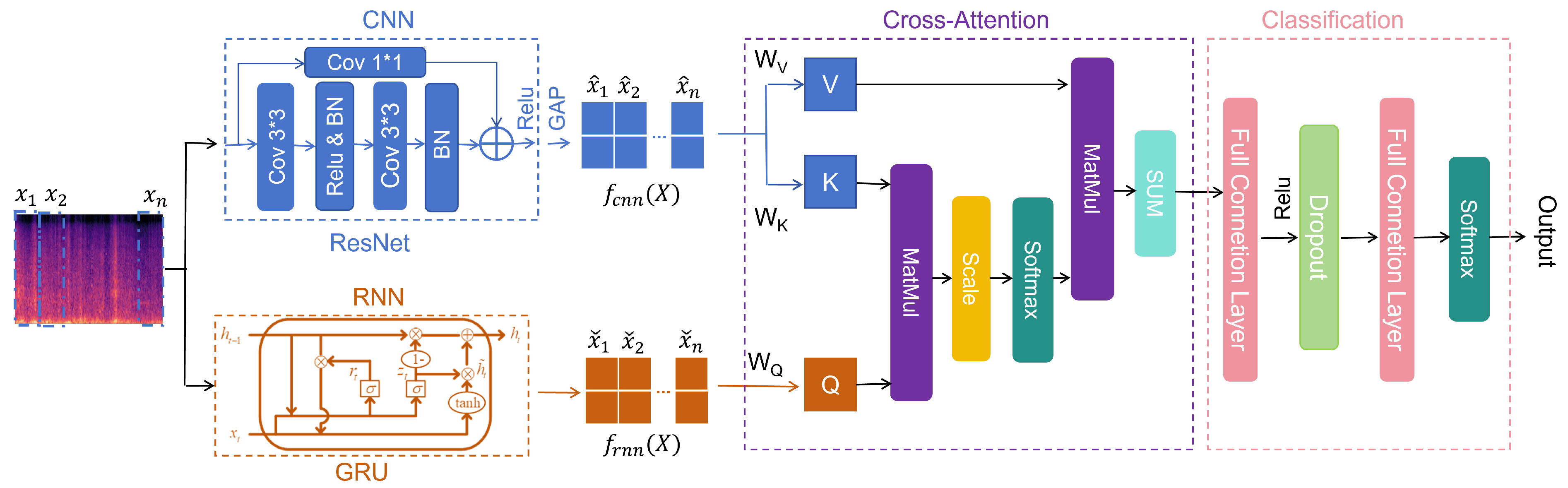
Figure 2.
Multiple events included in different time domains for spectrograms
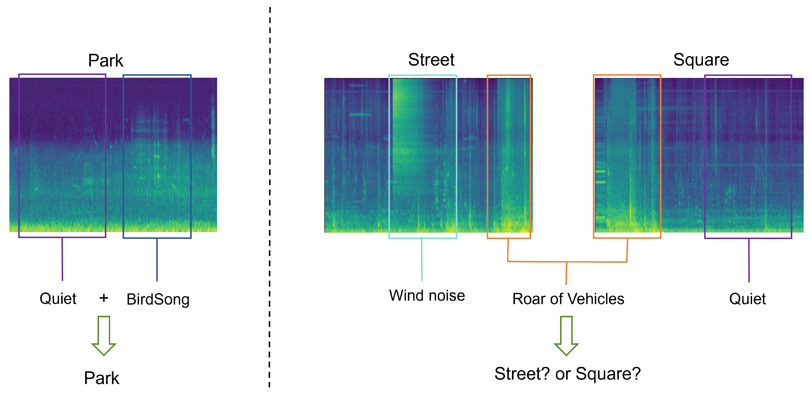
Figure 3.
Time segmentation on TUT2018
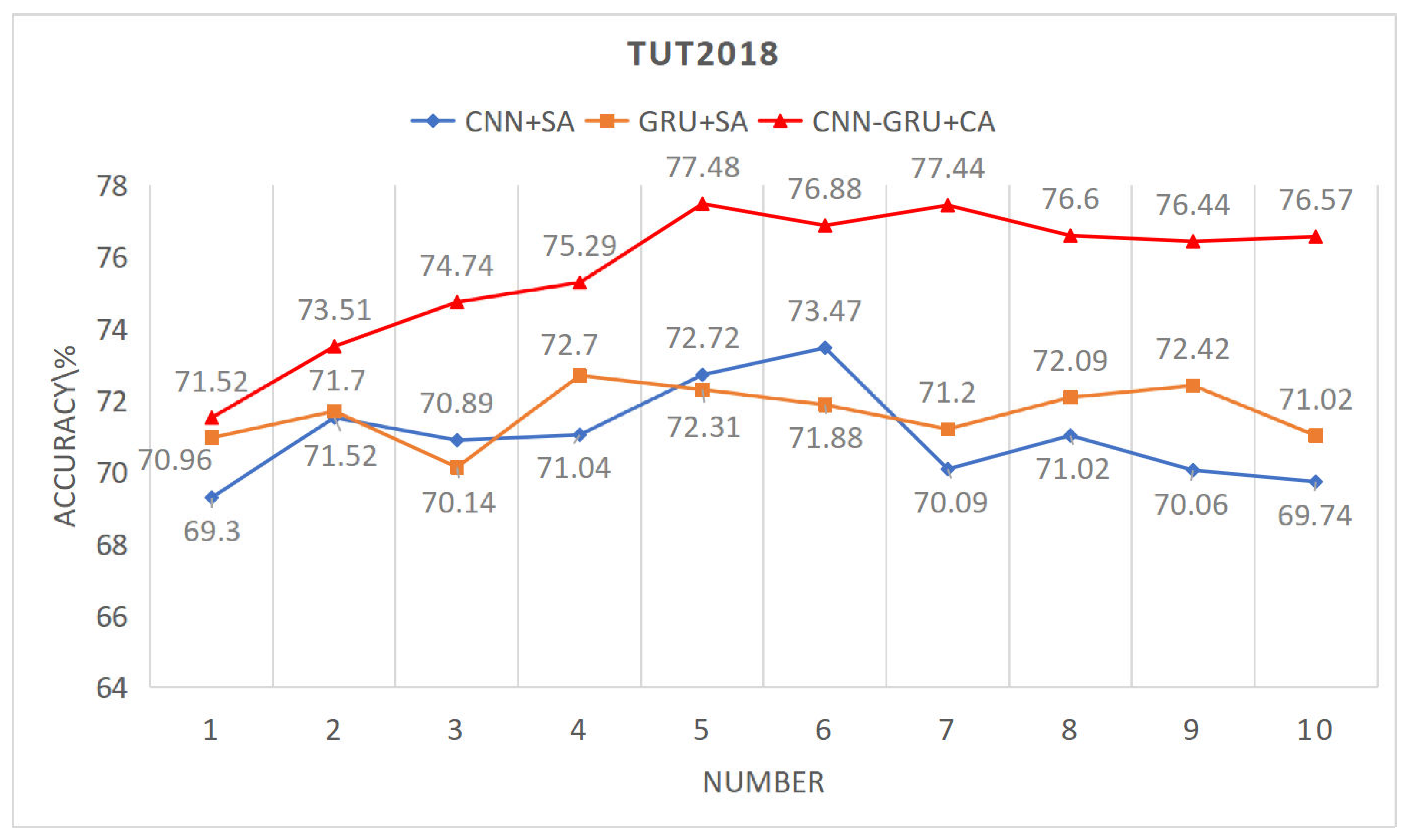
Figure 4.
Time segmentation on TAU2019
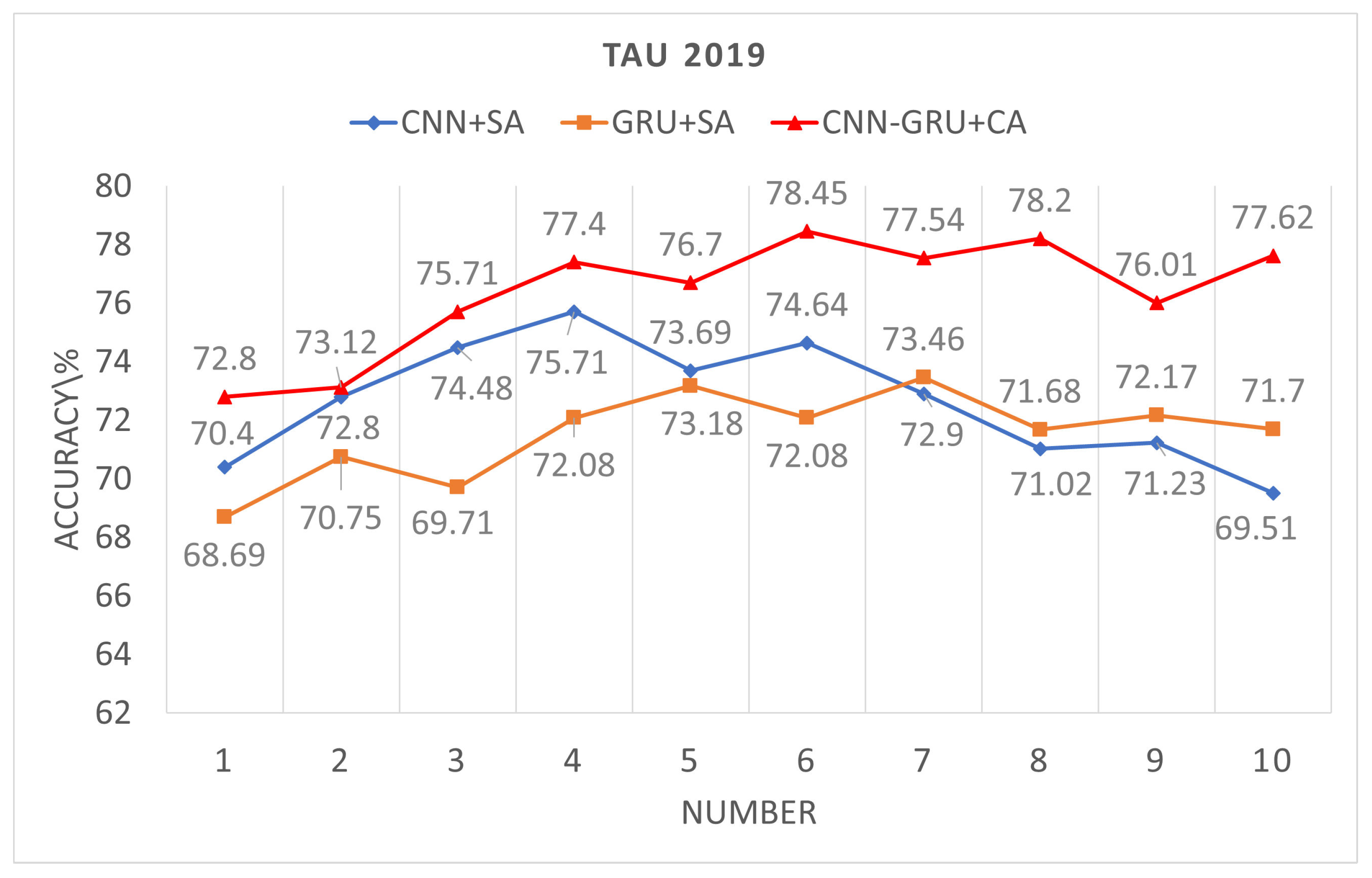
Figure 5.
Time segmentation on TAU2020
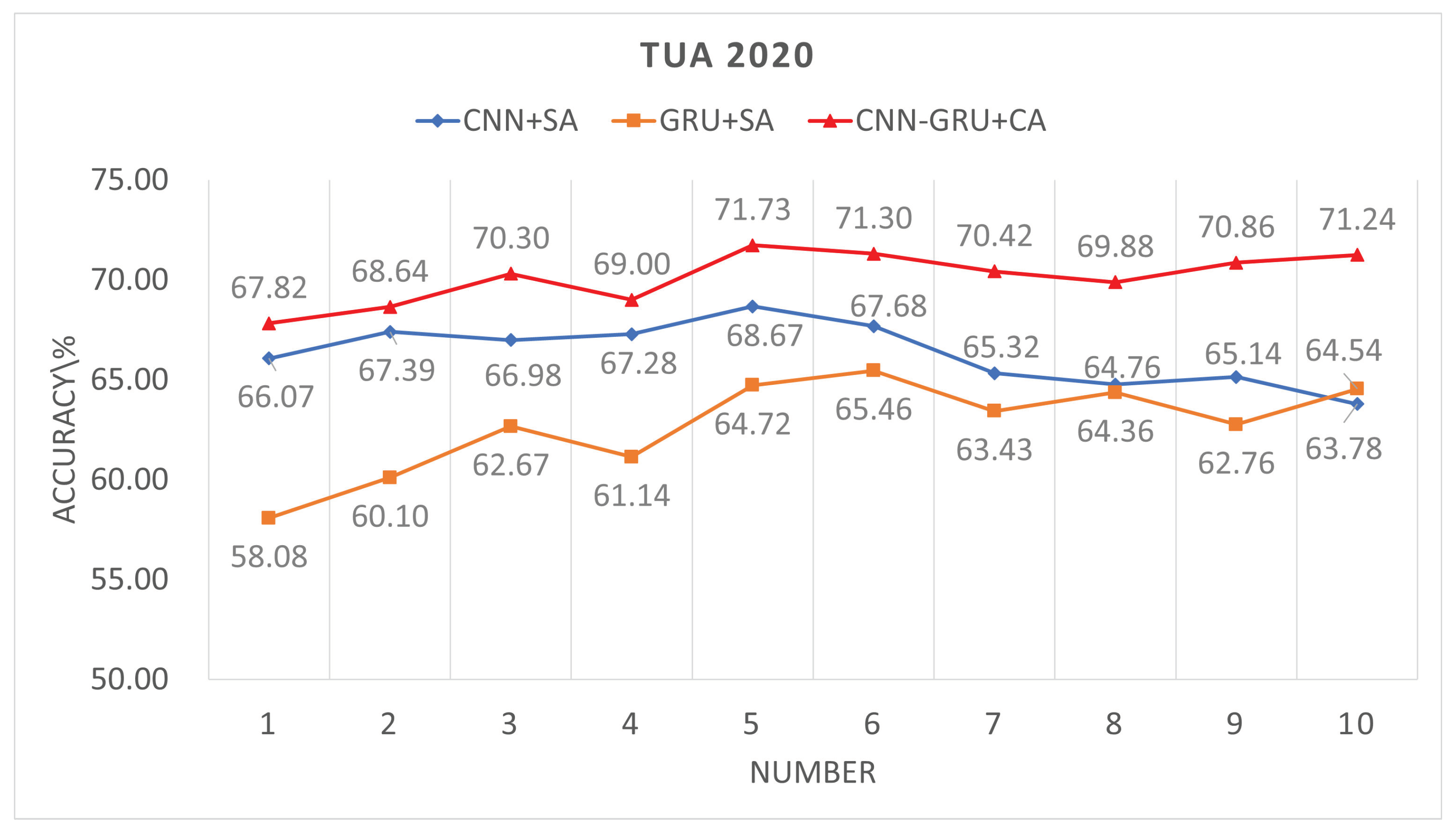

Table 1.
The results of different models.
| Model | TUT2018 | TAU2019 | TAU202020 |
|---|---|---|---|
| DCASE [19] | 59.7 | 62.5 | 51.6 |
| BiLSTM-CNN [15] | 73.6 | - | - |
| Visualfy [20] | - | 76.8 | - |
| MCTA-CNN [21] | 72.4 | 75.71 | - |
| LCNN [22] | - | - | 70.4 |
| VilEnsemb3 [23] | - | - | 70.3 |
| GA [24] | 76.7 | 78.2 | 71.3 |
| CNN+GRU+SA | 74.86 | 76.83 | 68.75 |
| GRU+CNN+SA | 73.92 | 76.26 | 68.06 |
| CNN-GRU+CO+SA | 75.34 | 77.38 | 69.86 |
| CNN-GRU+CA | 77.48 | 78.45 | 71.73 |
Disclaimer/Publisher’s Note: The statements, opinions and data contained in all publications are solely those of the individual author(s) and contributor(s) and not of MDPI and/or the editor(s). MDPI and/or the editor(s) disclaim responsibility for any injury to people or property resulting from any ideas, methods, instructions or products referred to in the content. |
© 2024 by the authors. Licensee MDPI, Basel, Switzerland. This article is an open access article distributed under the terms and conditions of the Creative Commons Attribution (CC BY) license (http://creativecommons.org/licenses/by/4.0/).
Copyright: This open access article is published under a Creative Commons CC BY 4.0 license, which permit the free download, distribution, and reuse, provided that the author and preprint are cited in any reuse.


