Submitted:
13 December 2024
Posted:
13 December 2024
You are already at the latest version
Abstract
AmeriFlux is a network of hundreds of sites across the contiguous United States providing tower-based ecosystem-scale carbon dioxide flux measurements at 30 minute temporal resolution. While geographically wide-ranging, over its existence the network has suffered from multiple issues including towers regularly ceasing operation for extended periods and a lack of standardization of measurements between sites. In this study, we address these issues by comparing seven machine learning algorithms to predict CO2 flux measurements using 35 environmental drivers and site-specific variables as predictors. We found that Extreme Gradient Boosting (XGBoost) consistently produced the most accurate predictions (Root Mean Squared Error of 1.81μmolm−2s−1, R2 of 0.86). The model showed excellent performance testing on sites that are ecologically similar to other sites (the Mid Atlantic, New England, and the Rocky Mountains), and poorer performance at sites with fewer ecological similarities to other sites in the data (Pacific Northwest, Florida, and Puerto Rico). The results show strong potential for machine learning-based models to make more skillful predictions than state-of-the-art process-based models, being able to estimate the multi-year mean carbon balance to within an error ± 50gCm−2y−1 for 29 of our 44 test sites. These results have significant implications for being able to accurately predict the carbon flux or gap-fill an extended outage at any AmeriFlux site, and for being able to quantify carbon flux in support of natural climate solutions.
Keywords:
Carbon dioxide flux
; nature-based climate solutions
; machine learning
; XGBoost
; National Ecological Observatory Network
; Ameriflux
; phenocam
1. Introduction
Tower-based, ecosystem-scale CO2 flux measurements quantify the exchange of turbulence flux of CO2 (FCO2, measured in molm−2s−2) between the land surface and the atmosphere. Plainly, FCO2 measures how much CO2 is moving into or out of an ecosystem, per unit area and per unit time. During daytime hours, most ecosystems are a strong sink for CO2 (negative FCO2, following the micrometeorological sign convention), as they remove CO2 from the atmosphere through the process of photosynthesis. By comparison, during the night, ecosystems are generally a moderate source of CO2 (positive FCO2), as they release CO2 back into the atmosphere through the process of respiration. FCO2 is measured using a method known as eddy covariance (EC) [3]. Eddy covariance measurements are continuous in time (24 hours a day, 7 days a week, 365 days a year) and are generally reported at an hourly or half-hourly temporal resolution. Global networks of eddy covariance flux towers collect in situ carbon flux measurements, providing information on photosynthesis dynamics across different ecosystems and under various environmental conditions.
Currently, FCO2 is measured at hundreds of research sites across the United States, with 385 of these sites being members of the AmeriFlux Network [9,34]. While these measurements run continuously at high frequency (e.g. at 5 Hz), practical limitations such as technical failures, instrument malfunction, and the necessity for filtering out data with low turbulent conditions have lead to extended gaps in the collected data. Moreover, there is no attempt to standardize the measurements across sites within the AmeriFlux network, meaning that when measurements are available, they may be more or less reliable than another site. Together, these compromise the validity of the fluxes that are measured and reported without issue.
These are the issues we tackle in this paper: developing a consistent, robust, and explainable method for quantifying FCO2. To do this we experiment with seven machine learning algorithms and 37 explanatory variables (environmental `drivers’) to make predictions about the half-hourly, daily, and annual FCO2 in 19 different ecosystems across the continental United States. In particular, our contributions can be summarized as follows:
- A wide-ranging comparison of many common machine learning methods for predicting tower-based FCO2;
- The discovery of a generalizable machine learning-based model that can predict FCO2 to within 1.81molm−2s−1 of tower-based measurements;
- An open source gap-filled FCO2 dataset covering 44 unique sites for free use by other researchers in the climate science community; and
- An open source code repository for reproducibility and wider implementation.
The remainder of the paper is organized as follows: Section 2 describes the background and purpose of the AmeriFlux Network, and provides the reader an explanation of the importance of quantifying carbon fluxes to the theory of Natural Climate Solutions; Section 3 discusses the state of existing work using machine learning for modeling CO2 and other flux measurements; Section 4 details the data, algorithms, and structure of our experiments, while the results are presented in Section 5 and they are analyzed further in Section 6; finally, we draw conclusions, discuss limitations, and suggest future directions in Section 7.
2. Background Information
2.1. The AmeriFlux network
The driving motivation for the establishment of AmeriFlux almost three decades ago was to measure the carbon balance of different ecosystems, and more specifically, to better understand the distribution of CO2 sinks and sources across the continent [49]. While this is an ambitious goal, from this perspective, the sampling provided by AmeriFlux is woefully inadequate–assuming that all 385 AmeriFlux sites are currently active (which they often are not), this coverage equates to approximately 1 flux measurement site every 25,000 km2.
Therefore, extrapolation and upscaling from individual sites to fine resolutions and regional and continental scales must be done using either process-based or statistically-based models. The former approach is attractive because these simulation models are based on state-of-the-art understanding of how the carbon cycle works. However, parameterization and initial conditions remain outstanding challenges, and past model validation efforts have highlighted serious model errors. By comparison, the latter approach is unattractive because many of these statistical approaches are essentially black boxes from which it is impossible to verify process-level representation. Standardization of inputs for statistical models is also a challenge, and, to the best of our knowledge, validation of model predictions has generally not been conducted against independent datasets.
An extensive model-data comparison project of over 20 ecosystem models conducted under the North American Carbon Program found that process-based models generally performed poorly in representing site-level carbon flux dynamics across sites with varying land cover. Specifically, substantial model errors in representing FCO2 were found at annual, seasonal, and diurnal time scales [10,44]; models misrepresented the inter-annual variability in observed CO2 uptake [25]; models did not properly represent phenological transitions in Spring or Fall [37]; and models could not predict photosynthetic uptake within the uncertainty of observations [42]. These results lead to valid questions about the viability of using process-based models to evaluate natural climate solution strategies (discussed later in Section 6).
Statistically-based upscaling of FCO2 began about two decades ago with the pioneering work of Papale et al. [35]. They used an artificial neural network, trained with CO2 flux data from 16 measurement sites in Europe to calibrate a simulation model to predict CO2 fluxes of European forests at 1 km resolution. Several years later, Xiao et al. [53] calibrated a modified regression tree model to FCO2 measurements across the AmeriFlux network, using satellite observed greenness indicators, such as vegetation indices, leaf area index, and fraction of observed photosynthetically active radiation [24]. The sophistication of these kinds of upscaling efforts has matured over the last 15 years. The current state of the art is probably defined by the FLUXCOM project [23], which uses satellite remote sensing and gridded meteorological products to calibrate a model trained on FCO2 measurements from sites around the world.
However, a challenge with past efforts to upscale site-level measurements is the lack of standardization in measurement protocols across sites. For example, across the AmeriFlux network, the choice of instrument setup and configuration, and even the details of flux data processing and corrections (which are critically important), may be different for each site. Furthermore, key instrumentation principles (e.g., open vs. closed path gas analyzer or sonic anemometer geometry), installation protocols (e.g., depth profiles of soil temperature and moisture measurements), measured and calibrated quantities (gravimetric vs. volumetric soil water content vs. soil water potential), and even units (hPa vs. kPa for vapor pressure deficit – easily converted, but also easily incorrectly reported or interpreted) are not consistent across sites. In particular, this lack of consistency of site variables across sites is a major barrier for any predictive modeling methods that use machine learning techniques.
The aforementioned inconsistency and variation in the AmeriFlux network’s data largely stems from its design as a “coalition of the willing”, where sites are setup and monitored by a large number of researchers (and consequently, research interests). Fortunately, FCO2 data from the 47 long-term research sites operated within the National Ecological Observatory Network (NEON) are also contributed to the AmeriFlux data archive. NEON was specifically established to “collect long-term open access ecological data to better understand how U.S. ecosystems are changing” [4], and implicit in this mission statement is the need for standardization of measurement protocols and techniques across sites. This standardization opens up the possibility to use a machine learning algorithm to predict site-level FCO2 without relying on gridded or reanalysis products as is necessary when using sites from AmeriFlux as a whole. Thus, the network of NEON sites represents an opportunity to train models on observational data across numerous sites which might be viewed as analogous to a model emulator [16]. The key difference being that this model is trained on real observations rather than the output of a simulation model.
NEON sites are strategically located, following a clustering algorithm to identify and group distinct regions of vegetation, landforms, and ecosystem dynamics into 20 different domains, as shown in Figure 1. Within each domain, at one or more monitoring sites, standardized measurements of environmental drivers (weather, solar radiation, etc.) are conducted along with ecosystem-level measurements of FCO2 and other quantities measured by eddy covariance (e.g. sensible and latent heat fluxes).
As discussed in Section 4, our experiments leverage the reliability, consistency, and high quality of the data collected at NEON-based AmeriFlux sites to train machine learning models.
2.2. Natural Climate Solutions
Accurately quantifying the terrestrial-atmospheric exchange of carbon is vital to assessing the impact of environmental management projects and policies at all scales. Hemes et al. [19] argue that ecosystem-scale CO2 flux measurements can play an important role in developing and evaluating climate mitigation strategies at the global level, while Hollinger et al. [20] noted the value of CO2 flux measurements for quantifying the magnitude of carbon storage, on an annual basis, by a single evergreen forest. Both of these articles also highlight the value of accurate CO2 flux measurements in the context of a theory known as Natural Climate Solutions (NCS).
NCS is a framework for adapting existing theory and knowledge of ecosystem science to mitigate the impact of anthropogenic climate change. It focuses on deliberate actions to manage, restore, and otherwise conserve ecosystems, to increase the quantity of CO2 they remove from the atmosphere and store in slow-turnover carbon reservoirs, such as soil or woody biomass. While the role of terrestrial ecosystems in the global carbon cycle has been relatively well-understood for decades [43,52], the theory of NCS was first defined in 2017, in a presentation by a group of scientists and practitioners at the Proceedings of the National Academy of Sciences [17]. Since this time, support for natural climate solutions has gradually gained momentum [5,15], (potentially because efforts to reduce fossil fuel emissions have not yet been successful).
A recent work [13] defined the five foundational principles of NCS, with Principle 4 reading: `There are multiple potential NCS actions that can occur in a given landscape and quantifying the overall magnitude of opportunity can help to focus efforts on the actions that can offer the largest mitigation returns. However, appropriate accounting is required to ensure that NCS potential is consistently and clearly quantified.’ The authors argue that accurate carbon dioxide flux estimation is essential to the implementation and adoption of NCS, as it will help optimize the actions taking by governments and other land managers. The machine learning-based predictive modeling conducted in this paper aims to contribute to this important need.
3. Literature Review
The prediction of CO2 is an important task in environmental sciences as rising levels of atmospheric CO2 are the primary cause of climate change [26]. However, it is also a difficult predictive modeling problem, and relatively few studies have been conducted in this space, and even fewer using modern machine learning methods.
The majority of existing work using machine learning to predict CO2 is focussed on estimating the atmospheric CO2 concentration at various geographical scales (as opposed to our focus of predicting CO2 flux). Alomar et al. [1] used extreme learning machines (a variation of feed-forward neural networks) to accurately predict CO2 concentration based on a single site in Hawaii, while Hou et al. [21] used XGBoost to predict emissions in geographical regions of China. Conversely, Fang et al. [14] uses Gaussian processes, and Mardani et al. [31] uses a multi-stage neural network technique to predict national-level carbon emissions. A policy-based need for this modeling is evident in Zhang et al. [54], where a genetic algorithm was used to assess the impact of China’s ecological zones on its CO2 emissions. Finally, Baareh et al. [2] take a time series forecasting approach to modeling CO2 emissions with a neural network.
Model choice, hyperparameter tuning, and variable choice are always difficult in machine learning-based work, which is why Hamrani et al. [18] compared nine different machine learning algorithms to predict CO2 for their specific agricultural sites, and Durmanov et al. [12] looked at the key enablers of greenhouse gases.
When considering the prediction of eddy covariance carbon dioxide flux with machine learning, the existing research either produced a low accuracy model, or a model that cannot generalize beyond the experimental site/s. For example, Tramontana et al. [48] predicted carbon dioxide and energy fluxes across global FLUXNET sites with 4 different algorithms, but the R2 for net ecosystem exchange of CO2 was less than 0.5. Alternatively, multiple works [11,41,50,55] all demonstrate high accuracy results using machine learning models to predict carbon dioxide on single or few experimental sites.
While most gap-filling techniques are process-based, Zhou et al.[56] used a variation of a random forest model to gap-fill extra long periods of missing values in carbon, heat, and energy fluxes. For further reading, a survey on using machine learning to predict various air pollutants including CO2 is presented in [29].
4. Methods
Our experiments compared the performance of seven machine learning algorithms to predict half-hourly FCO2 measurements collected between January 1st, 2016 and June 30, 2022. The experimental details are all provided in the following section and the code for the experiments is available at: https://github.com/jsl339/AmeriFlux.
4.1. Data
There are 47 NEON core terrestrial sites located across the U.S. and Puerto Rico, which strategically represent a range of vegetation, climate, and ecosystems divided into 20 different ecological domains as shown in Figure 1. Our experiments used data collected at 44 sites, as three sites–Marvin Klemme Range Research Station (OAES), Mountain Lake Biological Station (MLBS), and Puu Makaala Natural Area Reserve (PUUM)–were removed from the analysis due to inconsistencies in predictor variables, missing flux measurements, and errors arising during preprocessing. With these sites removed, our 44 sites represented 19 out of the 20 ecological domains (see [32] for general information about the data product).
We preprocessed the data using the R package REddyproc, as is the standard approach for gap-filling and u* filtering of carbon flux values. We used the U50 threshold to filter our u* values.
Table 1 shows a general explanation and summary statistics for the environmental drivers that we used as feature variables to learn our models. The data were sourced from 3 locations: AmeriFlux, the Phenocam Network, and MODIS satellite imagery [39,45,49].
Each site was assigned both a primary and secondary vegetation type from the following categories:
- Agricultural (AG)
- Deciduous Broadleaf (DB)
- Evergreen Broadleaf (EB)
- Evergreen Needleleaf (EN)
- Grassland (GR)
- Shrub (SH)
- Tundra (TN)
After preprocessing, our final dataset consisted of 961,340 observations unevenly divided among the 44 NEON sites.
4.2. Experimental Design
We compared the predictive performance of seven machine learning algorithms (explained in Section 4.3 below) in two experimental scenarios. The experiments employ cross validation, a common tool in machine learning experiments to ensure generalizability of the results. It does this by `holding out’ some data (called a `fold’), training the model without it, and testing on the held-out data. This gives an unbiased estimate of how the model would have performed on unseen data. This process is then repeated and averaged for robustness. When the data are split at random into k folds, this is referred to as k-fold cross validation.
In the first experimental scenario, we performed 10-fold cross validation on the data. This means that the data were randomly divided into 10 folds, with each containing approximately 10% of the data. The models were then trained using 9 folds (90% of the available data) and tested on the remaining fold. This process was repeated so that each fold was used in the training set 9 times and appeared as the test set once (see Figure 2a for an illustrated explanation). The performance of each algorithm was reported as the average across the 10 different runs. We note that the data were divided into the same 10 folds for each predictive algorithm.
K-fold cross-validation is a common technique in the testing and comparison of machine learning algorithms as it removes selection bias (whether deliberate or not), and demonstrates the ability of the models to generalize to unseen data [40].
In the second experimental scenario, which we will refer to as Leave-one-site-out cross-validation (L1SO CV), we began by partitioning the data by site, resulting in 44 uneven groups of data. We then employed a similar process to scenario one, where the models were trained on all-but-one group and tested on the remaining group (an example is shown in Figure 2b). This was repeated so that each site was used as the test data once, and therefore the stated performance metrics are the average of the 44 models fitted and tested.
The L1SO CV experiments present an inherently more difficult problem than the prior scenario as a predictive model significantly benefits from learning from data belonging to the test site. These experiments were included to replicate a situation where a site has no prior carbon flux recordings, i.e. it could be a new site or the instrumentation might not be functioning correctly. In addition, this experimental setup also tests whether we might be able to make a minimal set of measurements at a site with lower standardization in measurement protocols in order to predict the FCO2. This would be helpful for carbon accounting purposes and nature-based carbon solutions, and also to enable a benchmark for land surface model simulations and checking existing datasets.
The performance of each model was assessed using 2 evaluation metrics—Root Mean Squared Error (RMSE) and the Coefficient of Determination (). The RMSE is the square root of the average of the squared prediction errors over all of the data in the test set. Specifically,
Where y is the measured (true) value and is the predicted value for a test set of size N. Due to the squared component of the metric, the RMSE is sensitive to large errors in any of the individual predictions.
The evaluation metric is a measure of the goodness-of-fit of the linear model found by regressing the predicted values against the true values. It is calculated as:
In contrast to RMSE, is not sensitive to large errors in any of the individual predictions as it measures the amount of total variance accounted for by the predictions. When used together, these metrics complement each other and provide a more comprehensive picture of the performance of the algorithms. Each metric can then be analyzed on half-hourly, daily, and annual timescales. Ensuring accurate model predictions on an annual scale is important for reliable carbon accounting. However, it is also critical to evaluate model performance at finer temporal resolutions, such as half-hourly and daily scales, to ensure that our models produce accurate annual predictions for scientifically sound reasons. In order to produce meaningful predictions of annual sums of FCO2 for each test site, we must first use models optimized in the 10-fold experimental setting to fill in missing FCO2 values for each site before making predictions per site in the L1SO experimental setting.
4.3. Machine Learning Models
We compared the performance of 6 different machine learning models on predicting carbon dioxide flux. They are:
- Linear Regression (all predictors): This is a linear model including all of the variables using the maximum likelihood estimates for the coefficients. Linear regression assumes a linear relationship between the predictors and the response variable, which is unlikely in complex modeling problems, but does provide a baseline for the comparison of the performance of other models.
- Stepwise Linear Regression: This model began by testing for the most significant single variable in a linear regression model, and then iteratively added variables and tested for greatest improvement. A threshold number of selection variables was set to 15 for this forward selection technique. In this way, we simplify the basic linear regression model to find feature variables with greater importance for linear prediction.
- Decision Tree: A decision tree is a model based on recursively splitting the data on values of variables to maximize the difference between observations. Decision trees are most effective on problems where there is a non-linear relationship between the predictors and response variable [33,51]. The optimal tree depth was found to be 10 which was found through cross-validation.
- Random Forest: A random forest model [7] is a bagged ensemble of decision trees. The algorithm creates an uncorrelated forest of decision trees by using random subsets of features in each tree. When predicting a regression variable with a random forest model, the overall prediction is the average of the results of each of its constituent trees.
- Extreme Gradient Boosting (XGBoost): The XGBoost model [8] is a boosted ensemble of n underfit decision tree models. In practice, a decision tree is fit the to data and the errors in prediction are measured. Next, a second decision tree is used to fit the errors of the first tree. Then a third decision tree is fit to the errors of the second tree, and we continue until we have n trees in our ensemble. The optimal number of trees in our ensemble was found to be 2000. We also set the number of rounds for early stopping to be 50, and we used a learning rate of 0.05, max depth of 10, subsample ratio of 0.5, and subsample ratio of columns for each node of 0.45. Finally we used the histogram-optimized approximate greedy algorithm for tree construction to optimize our XGBoost model. All hyperparameters were optimized through 10-fold cross-validation using an exhaustive grid search.
- Neural Network (single-layer): A neural network is the sum of weighted non-linear functions of the predictor variables. This model is a single-layer neural network, with 256 neurons in the hidden layer, and uses a feed-forward architecture with ReLU activation. Early stopping was implemented to prevent model over-fitting, and training was performed with a data loader with a batch size of 128. The learning rate was set to 0.0003, and the best performance was achieved with no weight decay using the Adam optimizer. For more information on the mathematics of neural networks, see: [22,30].
- Deep Neural Network: The model uses the same mathematical structure as the single-layer neural network, but increases the number of hidden layers to 3, each consisting of 256 neurons. Compared to the single-layer neural network, the increased depth of the model increases the number of parameters to learn, meaning the model is capable of modeling more complex relationships, but also takes longer to learn from the data.
5. Results
5.1. 10-Fold Cross-Validation Results
The results for fitting each model and testing on each fold of the 10-fold cross-validaiton experiments are shown in Table 2 (RMSE). The XGBoost model and deep Neural Network were the only two models with a RMSE less than 2molm−2s−1. The strength of these models suggests that there are non-linearities in the the relationships between the environmental drivers and FCO2. It is important to note that the XGBoost model outperformed our deep Neural Network at each stage throughout model development, and in addition the XGboost model requires significantly less training time than either neural network.
After determining the optimal algorithm, we used the trained XGBoost model to gap-fill all of the missing values for each of the 44 sites. The resulting dataset, consisting of 4,068,459 observations, is freely available at https://zenodo.org/records/10719776 for use by other researchers in the climate science community.
5.2. L1SO Cross-Validation Results
The results for fitting each model and testing on each site of the leave-one-site-out cross-validation experiments are shown in Table 3 (RMSE) and Table 4 (R2). Again, the XGBoost model was superior to all others with a mean prediction RMSE of 2.45molm−2s−1. This is 35% greater than the RMSE of same model in the 10-fold cross-validation experiments, demonstrating the substantial information the model gains from seeing data from the test site in the training set (as is the case in the 10-fold experiments).
The results also varied greatly between test sites–from a RMSE of 0.66molm−2s−1 up to 6.22molm−2s−1. The model performed best on Toolik (TOOL), as well as other sites with Tundra as the primary vegetation–Barrow Environmental Observatory (BARR), Healy (HEAL), and Niwot Ridge Mountain Research Station (NIWO)–suggesting that the environmental drivers for these sites are highly similar. Another justification for lower model RMSE across sites with Tundra primary vegetation is that these sites in general experience smaller magnitude fluxes. Random errors scale with flux magnitude, so it’s almost inevitable that sites with higher magnitude fluxes will have somewhat larger model-data mismatch.
The model performed worst on Lajas Experimental Station (LAJA), which is one of two sites in Puerto Rico, and together these two represent the only two sites with an evergreen broadleaf primary vegetation type. While we cannot separate the domain and primary vegetation effects here, we can say that our training data, which is mostly from the United States mainland, does not generalize well when predicting FCO2 in vastly different climates and ecosystems.
A map of the average RMSE per domain is shown in Figure 3.
5.3. XGBoost Feature Importance
The XGBoost algorithm has a built-in method for calculating the importance of each feature variable based on the amount that each feature’s split point improves model performance. A plot of the twenty most important features for prediction is shown in Figure 4.
There are two input features that are noticeably more important to the model than others–EVI and net radiation. This is interesting as these are not measurements taken through site-level instrumentation, which suggests that we can learn a lot about the FCO2 of a site just by knowing the vegetation greenness and the radiation environment of a site. Furthermore, six of the ten most important variables are continuous measurement variables, as opposed to the domain or vegetation categorical variables, meaning the model should generalize easier to any new sites of interest.
6. Discussion
6.1. Comparison of 10-fold and L1SO experimental results
By making predictions on each site in both 10-fold and L1SO contexts, we are able to gain greater understanding of model performance across the 44 NEON sites. We partitioned our model’s 10-fold RMSE by site, and treated a site’s average RMSE value as the irreducible error–that is, error that can be attributed to variability in the dataset, measurement errors, and the error inherent in using a model to predict a biological process. From there, we compare this irreducible error to the average RMSE values for each site obtained through L1SO CV experiments and therefore obtain an estimate of the amount of error attributable to testing on an `unseen’ sight, which we call the L1SO Remainder. A visualization of the baseline error and its corresponding L1SO remainder for each site, ordered by ecological domain, is shown in Figure 5.
The L1SO remainder gives us a reasonable way to identify sites that are difficult to predict without having that site’s data available in the training set. We identified five NEON terrestrial sites that had a L1SO remainder greater than 0.85. These sites are Guanica Forest (GUAN), Lajas Experimental Station (LAJA), LBJ National Grassland (CLBJ), Disney Wilderness Preserve (DSNY), and Wind River Experimental Forest (WREF). There are several reasons that can justify why these sites in particular may be difficult for a model in a L1SO scenario. Firstly, Guanica Forest and Lajas Experimental Station are the only two sites in Puerto Rico and in ecological domain 4. In addition, these two sites are the only two whose primary vegetation type is evergreen broadleaf (EB).
Wind River Experimental Forest is a site in Washington state, located in an old growth forest with very tall trees with a real summer dry-down that restricts FCO2. Overall, Wind River Experimental Forest is a very unusual site in comparison with the other NEON terrestrial sites.
For each of these five sites, we created time series of predicted FCO2 values and actual FCO2values reported both in half hourly increments, and aggregated as an average for each day of the year, as well as a scatter plot of predicted FCO2 vs. actual FCO2 for analysis. We then compared these results to sites with the same primary vegetation types for which our model had superior performance. In the case of Guanica Forest and Lajas Experimental Station, since there were no other sites with the same primary vegetation type, both sites are included in Figure 6.
Steigerwaldt Land Services (STEI), Dakota Coteau Field School (DCFS), and Delta Junction (DEJU) were used as comparison for our other three sites representing primary vegetation types of DB, GR and EN respectively. These comparisons are found in Figure 7, Figure 8, and Figure 9.
Note that in most cases we observed large systematic errors in model performance for our 5 sites with the greatest L1SO Remainder values. For example, when considering scatterplots of predicted vs observed FCO2 for LAJA and WREF, the slope of predicted vs observed FCO2 is less than 1. At CLBJ, the magnitude of summertime uptake is under-predicted. At DSNY, the seasonality is represented well but there is a consistent offset of several molm−2s−1, with predicted values higher than measured values. By comparison, at STEI, DCFS, and DEJU, the magnitude and timing of predicted FCO2 is much better.
What is interesting from this analysis is that even on sites with relatively high L1SO remainder, our model seems to do a good job on average predicting patterns and dips in daily average FCO2. It appears that most of the errors associated with sites with large L1SO remainder can be attributed to the model being too conservative in its predictions, that is predicting values closer to zero than the true measured flux values. As seen by the right column of plots in Figure 7, Figure 8 and Figure 9, sites of the same primary vegetation type where our model had stronger performance seem to generally have less large positive and negative flux values. This makes sense, since our model learns to minimize prediction error, and since each error ends up being squared, predicting very large positive or negative values in general would be more heavily penalized. A good example of this fact can be seen in the half-hourly time series for Lajas Experimental Station in Figure 6. This site has a mix of large positive and negative observed flux values, and our model rarely made large positive or negative predictions. Compare this to a site like Delta Junction in Figure 8. Here, there are a number of large negative observed flux values, but not as many large positive values. Spikes in the negative direction are less erratic, and model predictions, as a result, more closely represented measured flux values. When looking at scatter plots of predicted flux vs. observed flux, one can see that the results for sites in the right hand column are more tightly clustered about the 1:1 line, resulting in higher scores.
6.2. Relevance of L1SO predictions for unseen sites
Historically, process-based models have been considered the “gold standard” for predicting ecosystem CO2 fluxes. However, past model-data evaluation studies have shown that although process-based models can often predict daily- or sub-daily fluxes that agree reasonably well with measured values, model performance on longer time scales (seasonal, annual and inter-annual) is often quite poor [10,25,47]. Models that cannot accurately predict ecosystem carbon budgets on annual and inter-annual time scales are not likely to be useful for carbon accounting purposes or for developing strategies for nature-based climate solutions. This suggests that alternatives to process-based models are needed. While machine learning-based models have been used for flux upscaling for almost two decades [23,35,53], these analyses have generally attempted to extrapolate from individual sites to regions and continents using only remotely-sensed variables as drivers. While this strategy is intuitively appealing, it is unable to leverage the site-level characteristics that are undoubtedly relevant for making fine-scale predictions. Indeed, basic ecosystem theory suggests that without accounting for these site-level characteristics such as disturbance and land use history, it is impossible to predict ecosystem carbon balance. Notably, we found that site characteristics related to vegetation type, as well as to soils, were identified as among the most important features for predicting FCO2. However, remotely-sensed variables from MODIS such as EVI and NDVI were found to be more important than site-level vegetation indices (e.g. Gcc, Rcc) derived from PhenoCam imagery. We can hypothesize that while PhenoCam imagery can provide phenological information at a fine spatial and temporal scale, it may be subject to issues related to the mismatch of footprints with eddy covariance flux measurements. In the case of heterogeneous landscapes, MODIS vegetation indices with larger spatial coverage may actually be more representative of seasonal variations in vegetation dynamics within the flux tower footprint.
Finally, we note that although site-level meteorological and environmental drivers (e.g. air temperature, relative humidity or VPD, soil temperature, soil moisture, and precipitation) were not ranked highly in terms of feature importance, this is not to say that these variables do not matter. Rather, it is likely that in the context of variation in FCO2 from the Arctic to the Tropics, from winter to summer, and from day to night, that the additional information contributed by these variables explains only a small amount of the half-hourly variation in FCO2, although it may contribute greatly to improved estimates of annual FCO2.
A persistent challenge in estimating site-level carbon balance via FCO2 measurements has always been that small but selectively systematic measurement errors in 30 minute data can accumulate to large errors in annual integrals [37]. In our machine learning approach, selectively systematic prediction errors could occur if important meteorological or environmental variables were not accounted for as covariates. Omission of these variables might do little to impact the calculated on 30 minute values but could seriously impact annual flux integrals. Adoption of model optimization criteria that place more weight on reducing selectively systematic bias (which might not even show up when bias is calculated over a multi-year dataset) and improving predictive power on annual and multi-year time scales could be important for further improving the application of machine learning methods to carbon accounting and nature-based climate solutions.
6.3. Leveraging Site-level Data when Standardized Model Inputs are not Available
Our feature importance plot (Figure 4) shows that, in spite of our assertion that site-level data are critical for correctly predicting ecosystem carbon balance, much of the information needed to predict half-hourly FCO2 actually comes from variables that are already available from gridded land cover maps (i.e. vegetation type classifications), satellite data products characterizing phenology (i.e. EVI, NDVI), and basic energy balance data that are also widely available as satellite data products (e.g., net radiation). This suggests that there is the potential for leveraging the much greater abundance of AmeriFlux towers, (for which site-level measurements are not standardized, but still useful), together with key remotely sensed data products to generate an initial map of ecosystem carbon balance. This initial map, when fused with elements of the analysis presented here, could lead to a hybrid data product that leverages the sampling intensity of AmeriFlux and the standardized sampling of NEON. Development of a data fusion platform such as we describe here is beyond the scope of the present analysis, but it is potentially an exciting direction to be pursued in future research.
6.4. Annual carbon sums
For most sites, we managed to obtain low RMSE and high R2 for predicting the measured half-hourly FCO2, even in the L1SO analysis (Table 3 and Table 4). However, in the context of carbon accounting and nature-based climate solutions, it more important to know the overall carbon balance on an annual time scale. That is, we want to answer the question of how much carbon (if any) the ecosystem is removing from the atmosphere and putting into biomass and soil carbon on an annual basis. This carbon balance reflects the balance between plant photosynthesis (carbon uptake, or negative flux) and ecosystem respiration (carbon release, or positive flux). It is a challenge for models, either process-based or data-driven, to get the overall carbon balance correct because of the opposing nature of these processes on different timescales. For example, in most ecosystems there is a strong seasonal pattern of carbon uptake during the growing season and release during the dormant season. During the growing season there is also a diurnal pattern of carbon uptake during the day and release during the night. Annually, the difference between photosynthesis and respiration is much smaller (0-30%) than the flux associated with either of these two key processes.
A model that predicts the annual carbon balance for an unknown site would be extremely valuable if it successfully estimated the multi-year mean carbon balance. The model would be even more useful it if successfully represented the inter-annual variability in carbon balance. State-of-the-art process-based models have generally failed to meet either of these targets [25]. Our results show that across all vegetation types, annual sums predicted in the L1SO analysis did a surprisingly good job at hitting the first target (see Table 5). For 29 out of 44 sites (66%), the L1SO-predicted multi-year mean carbon balance was within ± 50gCm−2y−1 of the “true” value estimated by gap-filling missing values in the CV analysis. This is quite remarkable given that the total uncertainty on the annual carbon balance, derived from gap-filled FCO2 measurements, is typically estimated to be about ± 50gCm−2y−1 [38]. However, for 7 of 44 sites (16%), the deviation between the L1SO-predicted multi-year mean and the “true” value was greater than 150gCm−2y−1. Three of these were deciduous broadleaf forest sites, one was an evergreen needleleaf forest site, and one was a grassland site. We expect that there may be land use history, disturbance, or similar factors that might explain these deviations, but were not included in our model.
Annual sums predicted in the L1SO analysis also did a reasonably good job of representing the “true” inter-annual variability estimated from gap-filled time series. At more than a quarter of sites (12 of 44, 27%), the correlation of L1SO-predicted annual sums and the gap-filled annual sums was greater than 0.75, while for almost half of sites (21 of 44, 47%) the correlation was greater than 0.50. While these results are based on at most 5 years of data per site, they point to the enormous potential of machine learning to predict not only the long-term carbon balance of an unknown site, but even the inter-annual variation in that carbon balance. By comparison, it has been known for more than a decade that even the most sophisticated process-based models are unable to capture this inter-annual variability [6,36,46], despite accurately capturing the dynamics of “fast” processes operating on timescales of hours to days.
7. Conclusions
In this paper we showed the ability of machine learning-based models to make skillful predictions of tower-based CO2 flux measurements. Specifically, we found that an XGBoost model trained on 37 environmental drivers, from 44 AmeriFlux sites, can predict FCO2 at an unseen site to within an average error of 2.45molm−2s−1. Furthermore, this error reduces significantly–down to as little as 0.66molm−2s−1–when a site in the training data has similar ecological characteristics to the unseen sites. This suggests that, with strategic placement of instrumentation to record future data, there is potential to predict most locations of interest with high accuracy. Our research underscores the importance of integrating advanced modeling techniques into carbon accounting frameworks, enabling more accurate quantification of carbon sequestration potential and guiding the implementation of effective natural climate mitigation strategies.
While our results are a significant step forward for quantifying carbon fluxes, we note that this work, like all machine learning-based modeling, is limited by the quality of the training data–the tower-based flux measurements. Both NEON flux measurements, and those from AmeriFlux more generally, have substantial uncertainties [38], but for the most part it is believed by the CO2 flux measurement community that theoretically-based corrections largely eliminate the systematic biases in measurements, and that the random errors then to average out over long time scales. Unfortunately, validating the accuracy of these measurements is a challenge because of all of the possible pathways by which CO2 can be removed from, stored, and returned to the atmosphere. Despite the lack of complete standardization across AmeriFlux sites, it is widely believed that tower-based measurements of FCO2 provide the most accurate and informative estimates of ecosystem carbon uptake and storage. Importantly, interpretation of annual FCO2 is also possible in a cross-site context, whereas it is not so straightforward to compare biometric forest inventory measurements with estimates of grassland productivity based on biomass clipping, or estimates of agricultural productivity based on crop yield. For this reason, the ability of our ML-based model to successfully predict across-site variation in annual FCO2 integrals, and within-site inter annual variation in annual FCO2 integrals, represents an important step forward in coast-to-coast mapping of ecosystem carbon balances, at fine spatial resolution, and the application of these carbon balance estimates in implementing natural climate solutions. Further improvements to our machine learning model (such as domain adaptation techniques [27,28]), using a wider range of data from across the AmeriFlux network, would undoubtedly be of value in advancing this socially-relevant field.
Author Contributions
Conceptualization, A.R. and B.L.; methodology, A.R. and B.L.; validation, J.U., J.L., and B.L.; formal analysis, J.U. and J.L.; resources, D.B., Y.L., and A.R.; data curation, J.U., J.L., D.B., and Y.L.; writing—original draft preparation, J.U., A.R., and B.L.; writing—review and editing, J.U., J.L., D.B., Y.L., A.R., and B.L.; project administration, A.R. and B.L.; funding acquisition, A.R. All authors have read and agreed to the published version of the manuscript.
Funding
This project was funded by NSF awards 1702697 and 2105828.
Data Availability Statement
All processed data and code is at https://github.com/jsl339/AmeriFlux. The gap-filled dataset has been made available for download at https://zenodo.org/records/10719776.
Conflicts of Interest
“The authors declare no conflict of interest.”
References
- AlOmar MK, Hameed MM, Al-Ansari N, Razali SFM, AlSaadi MA (2023) Short-, medium-, and long-term prediction of carbon dioxide emissions using wavelet-enhanced extreme learning machine. Civil Engineering Journal 9(4):815–834. [CrossRef]
- Baareh AK (2013) Solving the carbon dioxide emission estimation problem: An artificial neural network model. Journal of Software Engineering and Applications 6:338–342.
- Baldocchi DD (2020) How eddy covariance flux measurements have contributed to our understanding of global change biology. Global Change Biology 26(1):242–260.
- Battelle (2024) National Science Foundation’s National Ecological Observatory Network (NEON). https://www.neonscience.org/.
- Bossio D, Cook-Patton S, Ellis P, Fargione J, Sanderman J, Smith P, Wood S, Zomer R, Von Unger M, Emmer I, et al. (2020) The role of soil carbon in natural climate solutions. Nature Sustainability 3(5):391–398. [CrossRef]
- Braswell BH, Sacks WJ, Linder E, Schimel DS (2005) Estimating diurnal to annual ecosystem parameters by synthesis of a carbon flux model with eddy covariance net ecosystem exchange observations. Global Change Biology 11(2):335–355.
- Breiman L (2001) Random forests. Machine learning 45:5–32.
- Chen T, Guestrin C (2016) Xgboost: A scalable tree boosting system. In: Proceedings of the 22nd acm sigkdd international conference on knowledge discovery and data mining, pp 785–794.
- Chu H, Christianson DS, Cheah YW, Pastorello G, O’Brien F, Geden J, Ngo ST, Hollowgrass R, Leibowitz K, Beekwilder NF, et al. (2023) Ameriflux base data pipeline to support network growth and data sharing. Scientific Data 10(1):614. [CrossRef]
- Dietze MC, Vargas R, Richardson AD, Stoy PC, Barr AG, Anderson RS, Arain MA, Baker IT, Black TA, Chen JM, et al. (2011) Characterizing the performance of ecosystem models across time scales: A spectral analysis of the north american carbon program site-level synthesis. Journal of Geophysical Research: Biogeosciences 116(G4). [CrossRef]
- Dou X, Yang Y, Luo J (2018) Estimating forest carbon fluxes using machine learning techniques based on eddy covariance measurements. Sustainability 10(1):203.
- Durmanov A, Saidaxmedova N, Mamatkulov M, Rakhimova K, Askarov N, Khamrayeva S, Mukhtorov A, Khodjimukhamedova S, Madumarov T, Kurbanova K (2023) Sustainable growth of greenhouses: investigating key enablers and impacts. Emerging Science Journal 7(5):1674–1690.
- Ellis PW, Page AM, Wood S, Fargione J, Masuda YJ, Carrasco Denney V, Moore C, Kroeger T, Griscom B, Sanderman J, et al. (2024) The principles of natural climate solutions. Nature Communications 15(1):547. [CrossRef]
- Fang D, Zhang X, Yu Q, Jin TC, Tian L (2018) A novel method for carbon dioxide emission forecasting based on improved gaussian processes regression. Journal of cleaner production 173:143–150.
- Fargione JE, Bassett S, Boucher T, Bridgham SD, Conant RT, Cook-Patton SC, Ellis PW, Falcucci A, Fourqurean JW, Gopalakrishna T, et al. (2018) Natural climate solutions for the united states. Science Advances 4(11):eaat1869. [CrossRef]
- Fer I, Kelly R, Moorcroft PR, Richardson AD, Cowdery EM, Dietze MC (2018) Linking big models to big data: efficient ecosystem model calibration through bayesian model emulation. Biogeosciences 15(19):5801–5830.
- Griscom BW, Adams J, Ellis PW, Houghton RA, Lomax G, Miteva DA, Schlesinger WH, Shoch D, Siikamäki JV, Smith P, et al. (2017) Natural climate solutions. Proceedings of the National Academy of Sciences 114(44):11645–11650.
- Hamrani A, Akbarzadeh A, Madramootoo CA (2020) Machine learning for predicting greenhouse gas emissions from agricultural soils. Science of The Total Environment 741:140338.
- Hemes KS, Runkle BR, Novick KA, Baldocchi DD, Field CB (2021) An ecosystem-scale flux measurement strategy to assess natural climate solutions. Environmental science & technology 55(6):3494–3504.
- Hollinger D, Davidson E, Fraver S, Hughes H, Lee J, Richardson A, Savage K, Sihi D, Teets A (2021) Multi-decadal carbon cycle measurements indicate resistance to external drivers of change at the howland forest ameriflux site. Journal of Geophysical Research: Biogeosciences 126(8):e2021JG006276.
- Hou Y, Liu S (2024) Predictive modeling and validation of carbon emissions from china’s coastal construction industry: A bo-xgboost ensemble approach. Sustainability 16(10):4215.
- James G, Witten D, Hastie T, Tibshirani R (2021) An Introduction to Statistical Learning: with Applications in R: 2nd Edition. Springer, URL https://faculty.marshall.usc.edu/gareth-james/ISL/.
- Jung M, Schwalm C, Migliavacca M, Walther S, Camps-Valls G, Koirala S, Anthoni P, Besnard S, Bodesheim P, Carvalhais N, Chevallier F, Gans F, Goll DS, Haverd V, Köhler P, Ichii K, Jain AK, Liu J, Lombardozzi D, Nabel JEMS, Nelson JA, O’Sullivan M, Pallandt M, Papale D, Peters W, Pongratz J, Rödenbeck C, Sitch S, Tramontana G, Walker A, Weber U, Reichstein M (2020) Scaling carbon fluxes from eddy covariance sites to globe: synthesis and evaluation of the fluxcom approach. Biogeosciences 17(5):1343–1365.
- Kang Y, Gaber M, Bassiouni M, Lu X, Keenan T (2023) Cedar-gpp: spatiotemporally upscaled estimates of gross primary productivity incorporating co 2 fertilization. Earth System Science Data Discussions 2023:1–51.
- Keenan T, Baker I, Barr A, Ciais P, Davis K, Dietze M, Dragoni D, Gough CM, Grant R, Hollinger D, et al. (2012) Terrestrial biosphere model performance for inter-annual variability of land-atmosphere co2 exchange. Global Change Biology 18(6):1971–1987.
- Lee H, Calvin K, Dasgupta D, Krinner G, Mukherji A, Thorne P, Trisos C, Romero J, Aldunce P, Barret K, Blanco G, Cheung WW, Connors SL, Denton F, Diongue-Niang A, Dodman D, Garschagen M, Geden O, Hayward B, Jones C, Jotzo F, Krug T, Lasco R, Lee YY, Masson-Delmotte V, Meinshausen M, Mintenbeck K, Mokssit A, Otto FE, Pathak M, Pirani A, Poloczanska E, Pörtner HO, Revi A, Roberts DC, Roy J, Ruane AC, Skea J, Shukla PR, Slade R, Slangen A, Sokona Y, Sörensson AA, Tignor M, van Vuuren D, Wei YM, Winkler H, Zhai P, Zommers Z, Hourcade JC, Johnson FX, Pachauri S, Simpson NP, Singh C, Thomas A, Totin E, Arias P, Bustamante M, Elgizouli I, Flato G, Howden M, Méndez-Vallejo C, Pereira JJ, Pichs-Madruga R, Rose SK, Saheb Y, Rodríguez RS, Ürge-Vorsatz D, Xiao C, Yassaa N, Alegría A, Armour K, Bednar-Friedl B, Blok K, Cissé G, Dentener F, Eriksen S, Fischer E, Garner G, Guivarch C, Haasnoot M, Hansen G, Hauser M, Hawkins E, Hermans T, Kopp R, Leprince-Ringuet N, Lewis J, Ley D, Ludden C, Niamir L, Nicholls Z, Some S, Szopa S, Trewin B, van der Wijst KI, Winter G, Witting M, Birt A, Ha M, Romero J, Kim J, Haites EF, Jung Y, Stavins R, Birt A, Ha M, Orendain DJA, Ignon L, Park S, Park Y (2023) IPCC, 2023: Climate change 2023: Synthesis report, summary for policymakers. Contribution of working groups i, ii and iii to the sixth assessment report of the Intergovernmental Panel on Climate Change [H. Lee and J. Romero (eds.)]. IPCC, Geneva, Switzerland. Technical report, Intergovernmental Panel on Climate Change (IPCC), Geneva, Switzerland.
- Lucas B, Pelletier C, Inglada J, Schmidt D, Webb G I, and Petitjean F (2019) Exploring Data Quantity Requirements for Domain Adaptation in the Classification of Satellite Image Time Series. In: 10th International Workshop on the Analysis of Multitemporal Remote Sensing Images (MultiTemp), Shanghai, China, 2019, pp. 1-4.
- Lucas B, Pelletier C, Schmidt D, Webb G I, and Petitjean F (2020) Unsupervised Domain Adaptation Techniques for Classification of Satellite Image Time Series, In: IGARSS 2020 - 2020 IEEE International Geoscience and Remote Sensing Symposium, Waikoloa, HI, USA, 2020, pp. 1074-1077.
- Madan T, Sagar S, Virmani D (2020) Air quality prediction using machine learning algorithms –a review. In: 2020 2nd International Conference on Advances in Computing, Communication Control and Networking, pp 140–145.
- Mahabbati A, Beringer J, Leopold M, McHugh I, Cleverly J, Isaac P, Izady A (2021) A comparison of gap-filling algorithms for eddy covariance fluxes and their drivers. Geoscientific Instrumentation, Methods and Data Systems 10(1):123–140.
- Mardani A, Liao H, Nilashi M, Alrasheedi M, Cavallaro F (2020) A multi-stage method to predict carbon dioxide emissions using dimensionality reduction, clustering, and machine learning techniques. Journal of Cleaner Production 275:122942.
- National Ecological Observatory Network (2024) Bundled data products - eddy covariance (dp4.00200.001). URL https://data.neonscience.org/data-products/DP4.00200.001/RELEASE-2024.
- Nie F, Zhu W, Li X (2020) Decision tree svm: An extension of linear svm for non-linear classification. Neurocomputing 401:153–159.
- Novick KA, Biederman J, Desai A, Litvak M, Moore DJ, Scott R, Torn M (2018) The AmeriFlux network: A coalition of the willing. Agricultural and Forest Meteorology 249:444–456.
- Papale D, Valentini R (2003) A new assessment of european forests carbon exchanges by eddy fluxes and artificial neural network spatialization. Global Change Biology 9(4):525–535.
- Ricciuto DM, Davis KJ, Keller K (2008) A bayesian calibration of a simple carbon cycle model: The role of observations in estimating and reducing uncertainty. Global biogeochemical cycles 22(2).
- Richardson AD, Anderson RS, Arain MA, Barr AG, Bohrer G, Chen G, Chen JM, Ciais P, Davis KJ, Desai AR, et al. (2012a) Terrestrial biosphere models need better representation of vegetation phenology: results from the n orth a merican c arbon p rogram s ite s ynthesis. Global Change Biology 18(2):566–584.
- Richardson AD, Aubinet M, Barr AG, Hollinger DY, Ibrom A, Lasslop G, Reichstein M (2012b) Uncertainty quantification. In: Aubinet M, Vesala T, Papale D (eds) Eddy Covariance: A Practical Guide to Measurement and Data Analysis, Springer Netherlands, Dordrecht, pp 173–209.
- Richardson AD, Hufkens K, Milliman T, Aubrecht DM, Chen M, Gray JM, Johnston MR, Keenan TF, Klosterman ST, Kosmala M, et al. (2018) Tracking vegetation phenology across diverse north american biomes using phenocam imagery. Scientific data 5(1):1–24. [CrossRef]
- Rodriguez JD, Perez A, Lozano JA (2009) Sensitivity analysis of k-fold cross validation in prediction error estimation. IEEE transactions on pattern analysis and machine intelligence 32(3):569–575.
- Safaei-Farouji M, Thanh HV, Dai Z, Mehbodniya A, Rahimi M, Ashraf U, Radwan AE (2022) Exploring the power of machine learning to predict carbon dioxide trapping efficiency in saline aquifers for carbon geological storage project. Journal of Cleaner Production 372:133778.
- Schaefer K, Schwalm CR, Williams C, Arain MA, Barr A, Chen JM, Davis KJ, Dimitrov D, Hilton TW, Hollinger DY, et al. (2012) A model-data comparison of gross primary productivity: Results from the north american carbon program site synthesis. Journal of Geophysical Research: Biogeosciences 117(G3). [CrossRef]
- Schimel DS, House JI, Hibbard KA, Bousquet P, Ciais P, Peylin P, Braswell BH, Apps MJ, Baker D, Bondeau A, et al. (2001) Recent patterns and mechanisms of carbon exchange by terrestrial ecosystems. Nature 414(6860):169–172. [CrossRef]
- Schwalm CR, Williams CA, Schaefer K, Anderson R, Arain MA, Baker I, Barr A, Black TA, Chen G, Chen JM, et al. (2010) A model-data intercomparison of co2 exchange across north america: Results from the north american carbon program site synthesis. Journal of Geophysical Research: Biogeosciences 115(G3). [CrossRef]
- Seyednasrollah B, Young AM, Hufkens K, Milliman T, Friedl MA, Frolking S, Richardson AD (2019) Tracking vegetation phenology across diverse biomes using version 2.0 of the phenocam dataset. Scientific data 6(1):222.
- Siqueira M, Katul GG, Sampson D, Stoy PC, Juang JY, McCarthy HR, Oren R (2006) Multiscale model intercomparisons of co2 and h2o exchange rates in a maturing southeastern us pine forest. Global Change Biology 12(7):1189–1207.
- Stoy PC, Dietze MC, Richardson AD, Vargas R, Barr AG, Anderson RS, Arain MA, Baker IT, Black TA, Chen JM, Cook RB, Gough CM, Grant RF, Hollinger DY, Izaurralde RC, Kucharik CJ, Lafleur P, Law BE, Liu S, Lokupitiya E, Luo Y, Munger JW, Peng C, Poulter B, Price DT, Ricciuto DM, Riley WJ, Sahoo AK, Schaefer K, Schwalm CR, Tian H, Verbeeck H, Weng E (2013) Evaluating the agreement between measurements and models of net ecosystem exchange at different times and timescales using wavelet coherence: an example using data from the north american carbon program site-level interim synthesis. Biogeosciences 10(11):6893–6909.
- Tramontana G, Jung M, Schwalm CR, Ichii K, Camps-Valls G, Ráduly B, Reichstein M, Arain MA, Cescatti A, Kiely G, Merbold L, Serrano-Ortiz P, Sickert S, Wolf S, Papale D (2016) Predicting carbon dioxide and energy fluxes across global fluxnet sites with regression algorithms. Biogeosciences 13(14):4291–4313.
- United States Department of Energy (2023) AmeriFlux Management Project. https://ameriflux.lbl.gov/.
- Vais A, Mikhaylov P, Popova V, Nepovinnykh A, Nemich V, Andronova A, Mamedova S (2023) Carbon sequestration dynamics in urban-adjacent forests: a 50-year analysis. Civil Engineering Journal 9(9):2205–2220.
- Vanli ND, Sayin MO, Mohaghegh M, Ozkan H, Kozat SS (2019) Nonlinear regression via incremental decision trees. Pattern Recognition 86:1–13.
- Wofsy SC, Harris RC (2002) The north american carbon program 2002. Tech. rep., The Global Carbon Project, URL https://www.globalcarbonproject.org/global/pdf/thenorthamericancprogram2002.pdf.
- Xiao J, Zhuang Q, Baldocchi DD, Law BE, Richardson AD, Chen J, Oren R, Starr G, Noormets A, Ma S, et al. (2008) Estimation of net ecosystem carbon exchange for the conterminous united states by combining modis and ameriflux data. Agricultural and Forest Meteorology 148(11):1827–1847. [CrossRef]
- Zhang Y, Fu B (2023) Impact of china’s establishment of ecological civilization pilot zones on carbon dioxide emissions. Journal of Environmental Management 325:116652.
- Zhao J, Lange H, Meissner H (2022) Estimating carbon sink strength of norway spruce forests using machine learning. Forests 13(10):1721.
- Zhu S, Clement R, McCalmont J, Davies CA, Hill T (2022) Stable gap-filling for longer eddy covariance data gaps: A globally validated machine-learning approach for carbon dioxide, water, and energy fluxes. Agricultural and Forest Meteorology 314:108777.
Figure 1.
A map of the NEON core terrestrial sites and their locations within the 19 ecological domains.
Figure 1.
A map of the NEON core terrestrial sites and their locations within the 19 ecological domains.
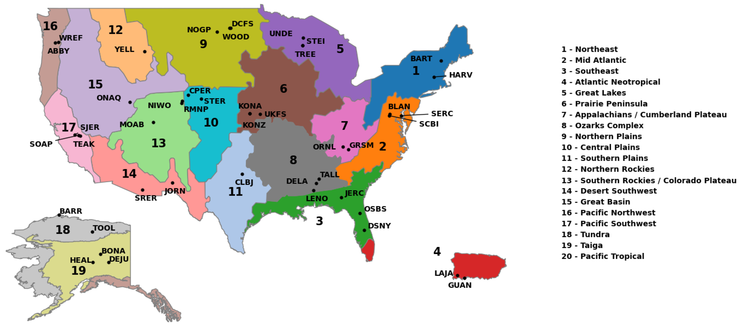
Figure 2.
A visual explanation of the cross-validation techniques used in our experiments. (a) illustrates the data split into 10 random `folds’ with the model being trained on 9 folds, and the tenth held-out for testing. This process is repeated 10-times and the results are averaged. (b) illustrates the data stratified by site, in this case the model is trained on all-but-one site, and this is held-out for testing. This is repeated until each site has been held-out as the test site exactly once.
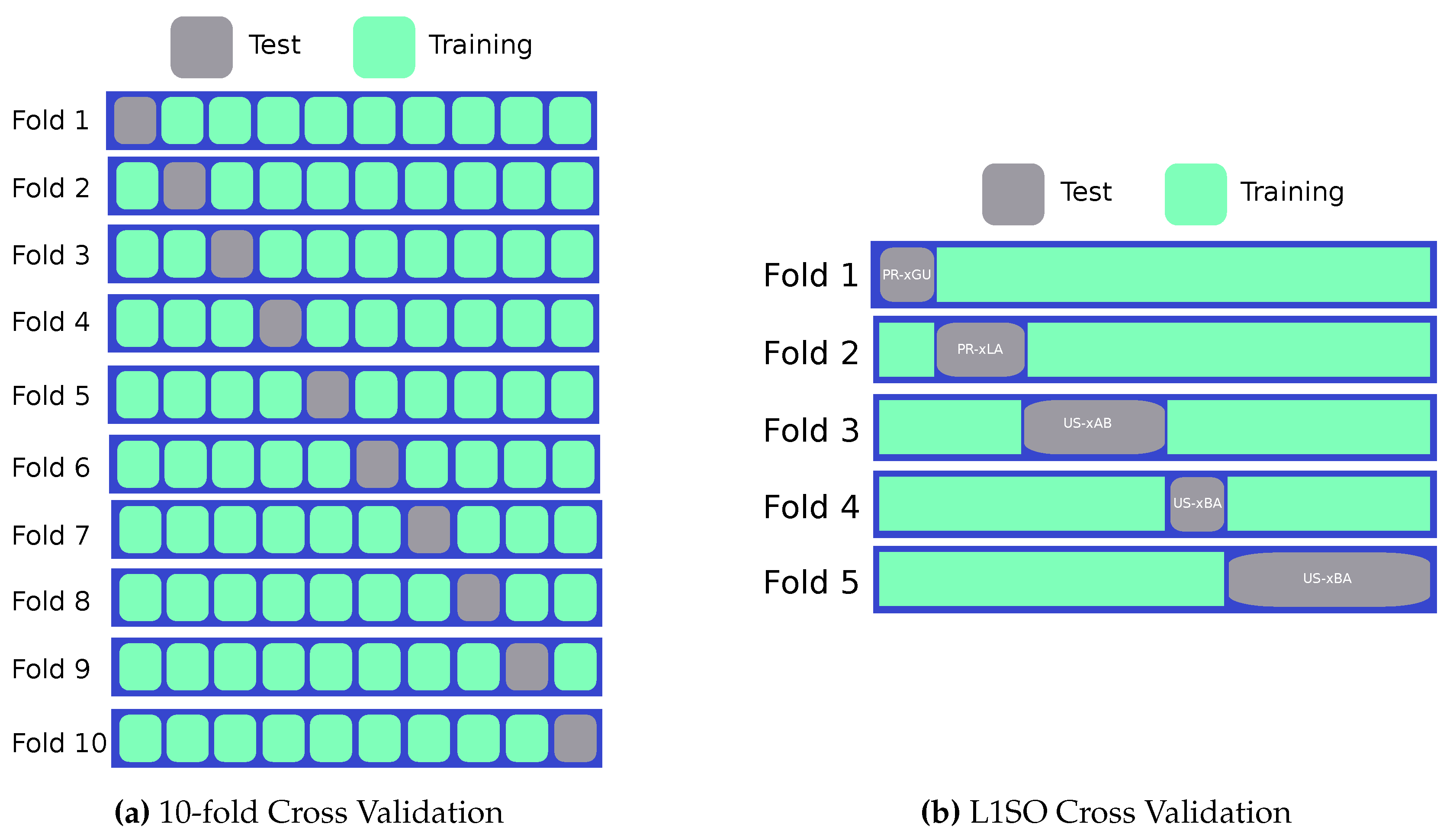
Figure 3.
The average RMSE (molm−2s−1) per domain for the leave-one-site-out experiments.
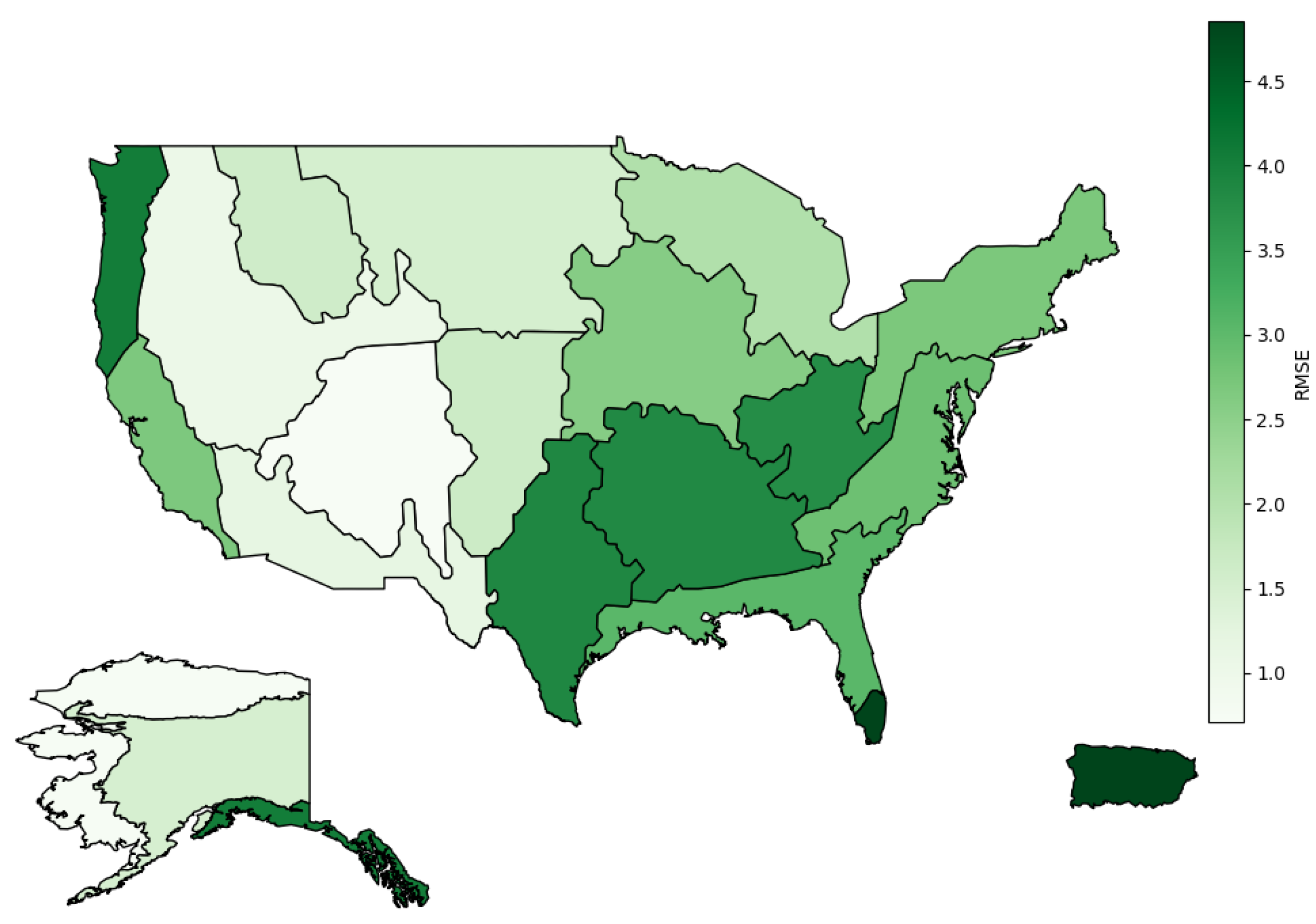
Figure 4.
The twenty most important features of our XGBoost model
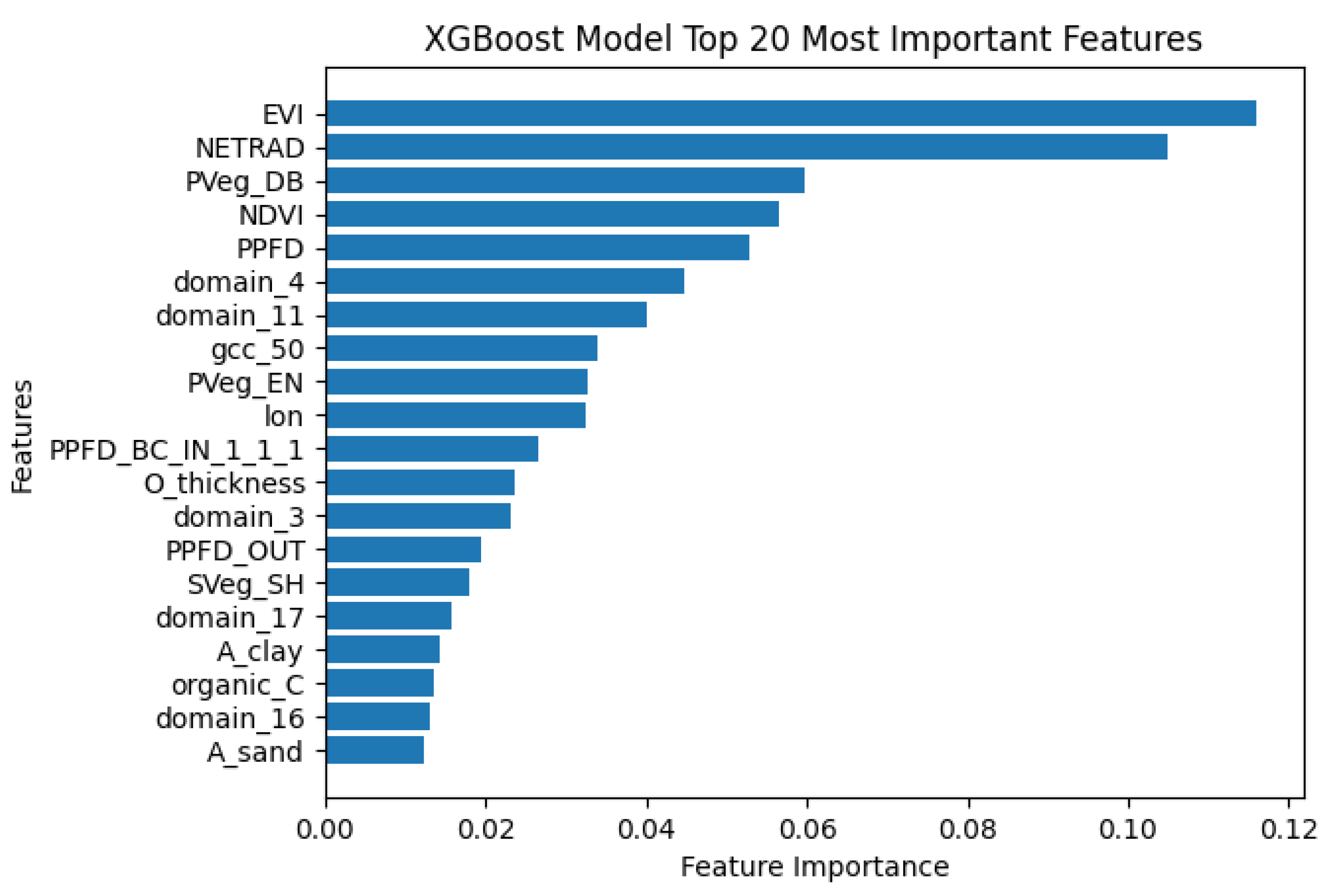
Figure 5.
Visualization of XGBoost L1SO RMSE remainder organized by domain number (shown as a prefix to the site code)
Figure 5.
Visualization of XGBoost L1SO RMSE remainder organized by domain number (shown as a prefix to the site code)
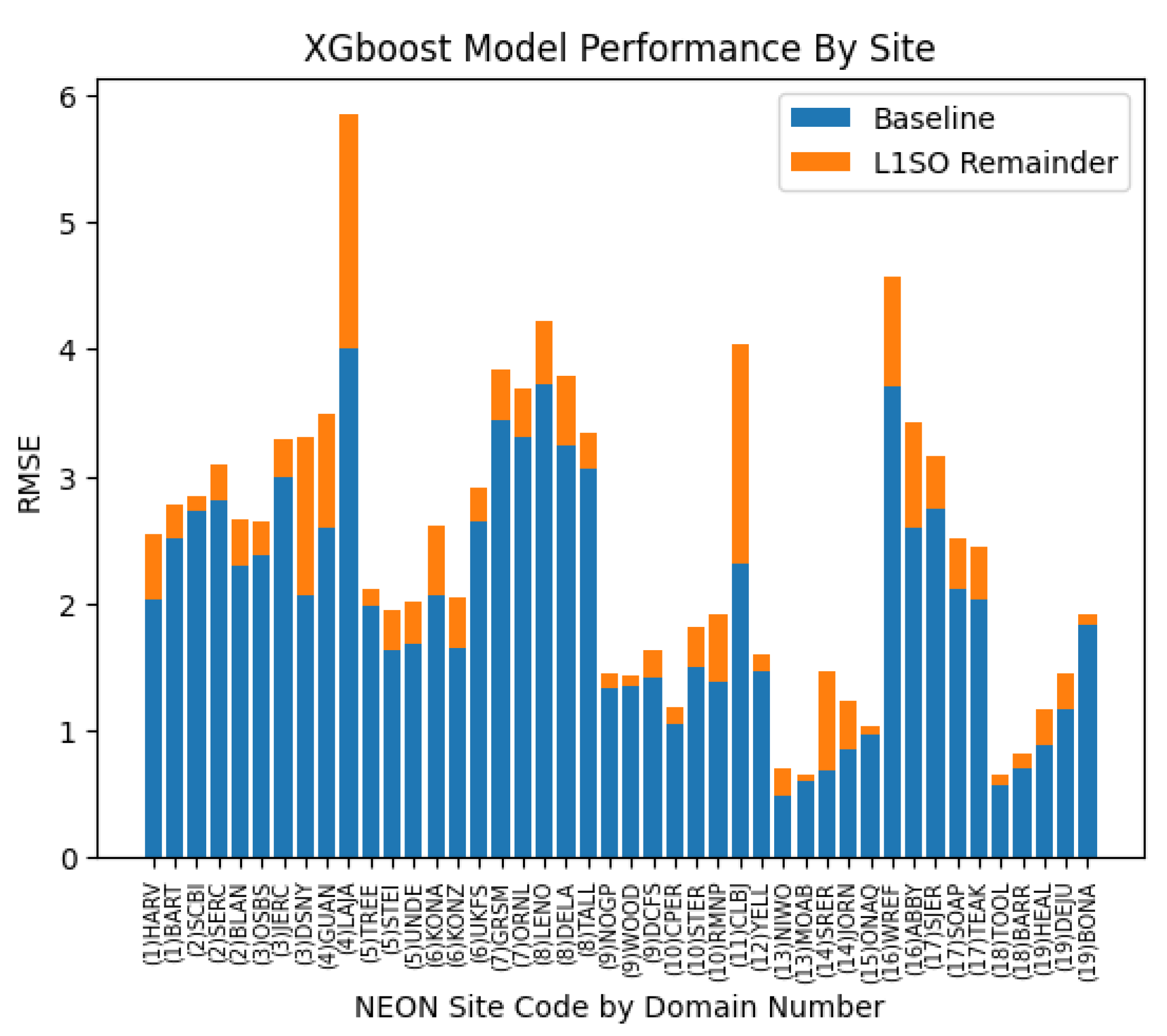
Figure 6.
Time series and scatter plots of FCO2 prediction error for sites with EB primary vegetation type
Figure 6.
Time series and scatter plots of FCO2 prediction error for sites with EB primary vegetation type
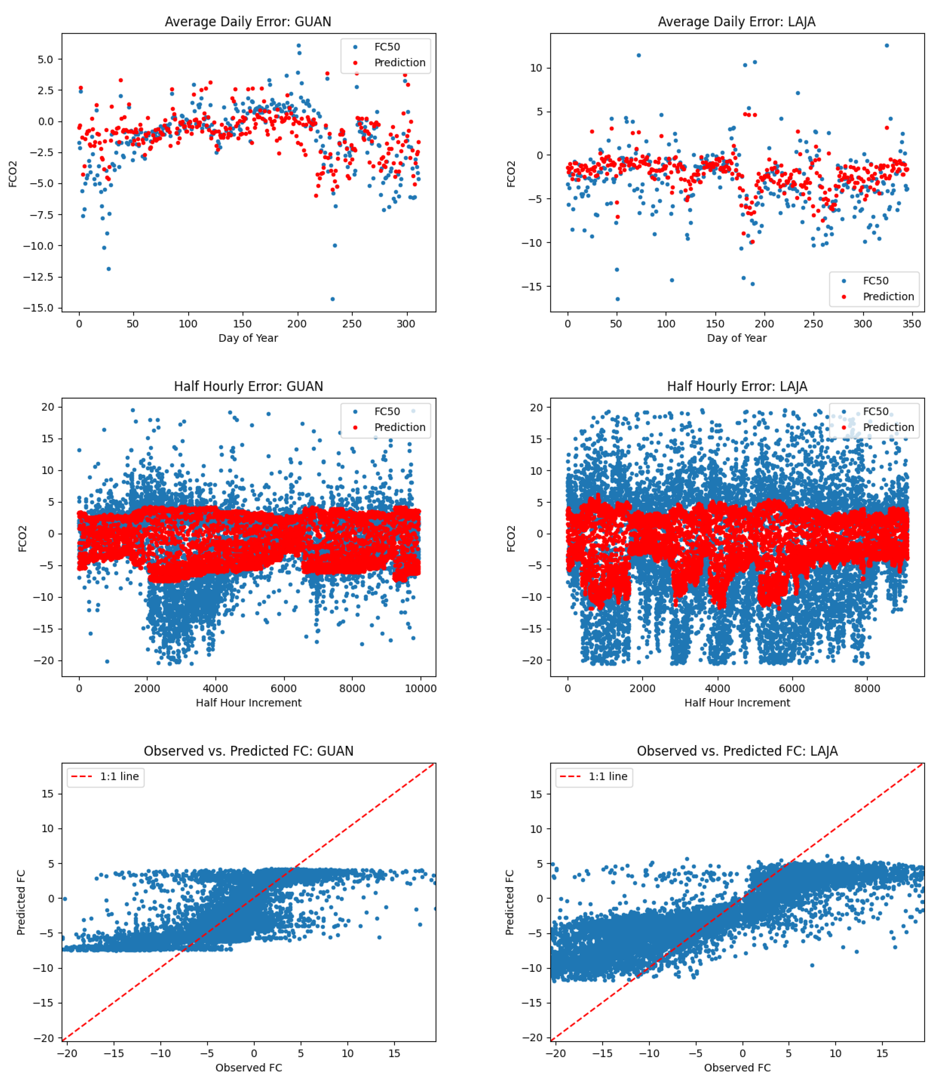
Figure 7.
Comparison of FCO2 prediction error for sites with DB primary vegetation type. Site with poor model performance (CLBJ) is on the left and site with better model performance (STEI) on the right.
Figure 7.
Comparison of FCO2 prediction error for sites with DB primary vegetation type. Site with poor model performance (CLBJ) is on the left and site with better model performance (STEI) on the right.
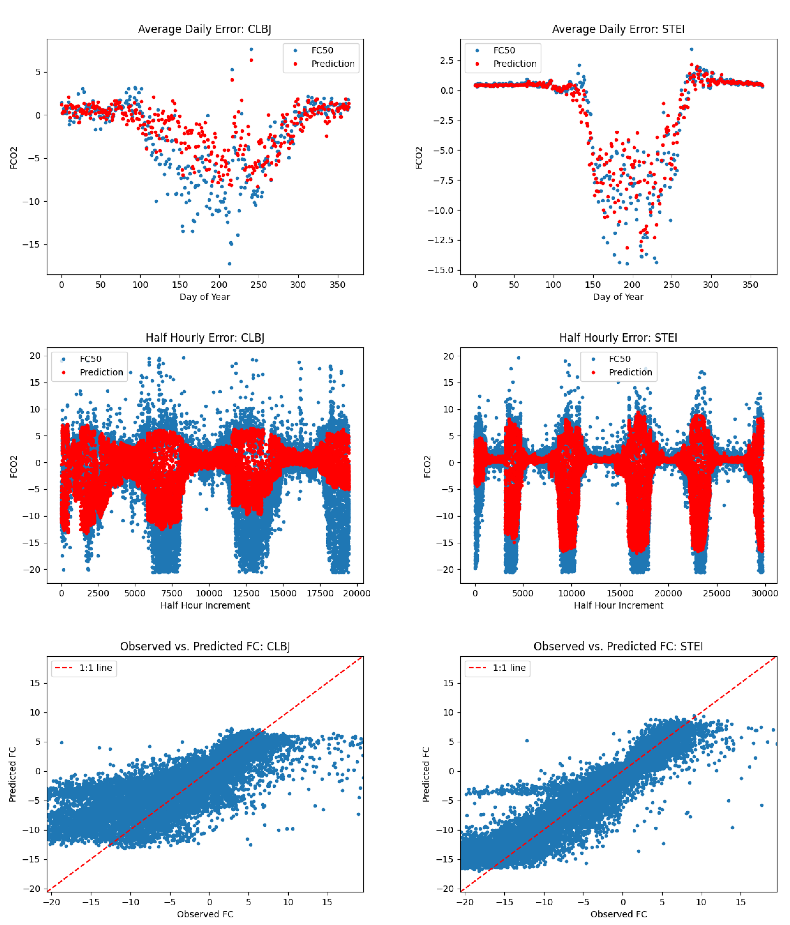
Figure 8.
Comparison of FCO2 prediction error for sites with GR primary vegetation type. Site with poor model performance (DSNY) is on the left and site with better model performance (DCFS) on the right.
Figure 8.
Comparison of FCO2 prediction error for sites with GR primary vegetation type. Site with poor model performance (DSNY) is on the left and site with better model performance (DCFS) on the right.
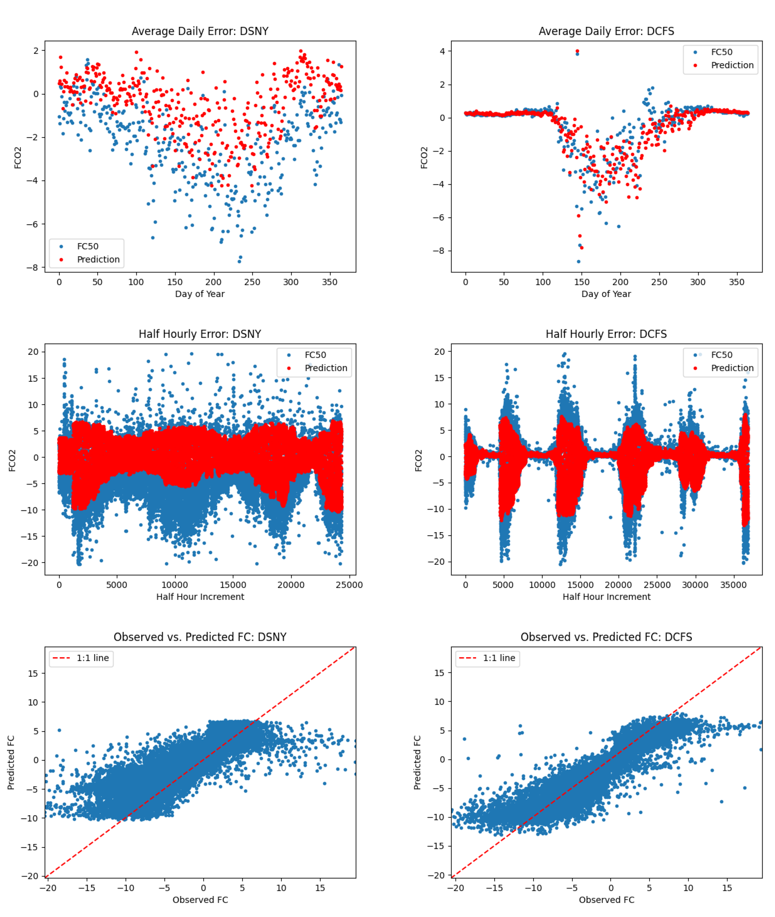
Figure 9.
Comparison of sites with EN primary vegetation type. Site with poor model performance (WREF) is on the left and site with better model performance (DEJU) on the right.
Figure 9.
Comparison of sites with EN primary vegetation type. Site with poor model performance (WREF) is on the left and site with better model performance (DEJU) on the right.
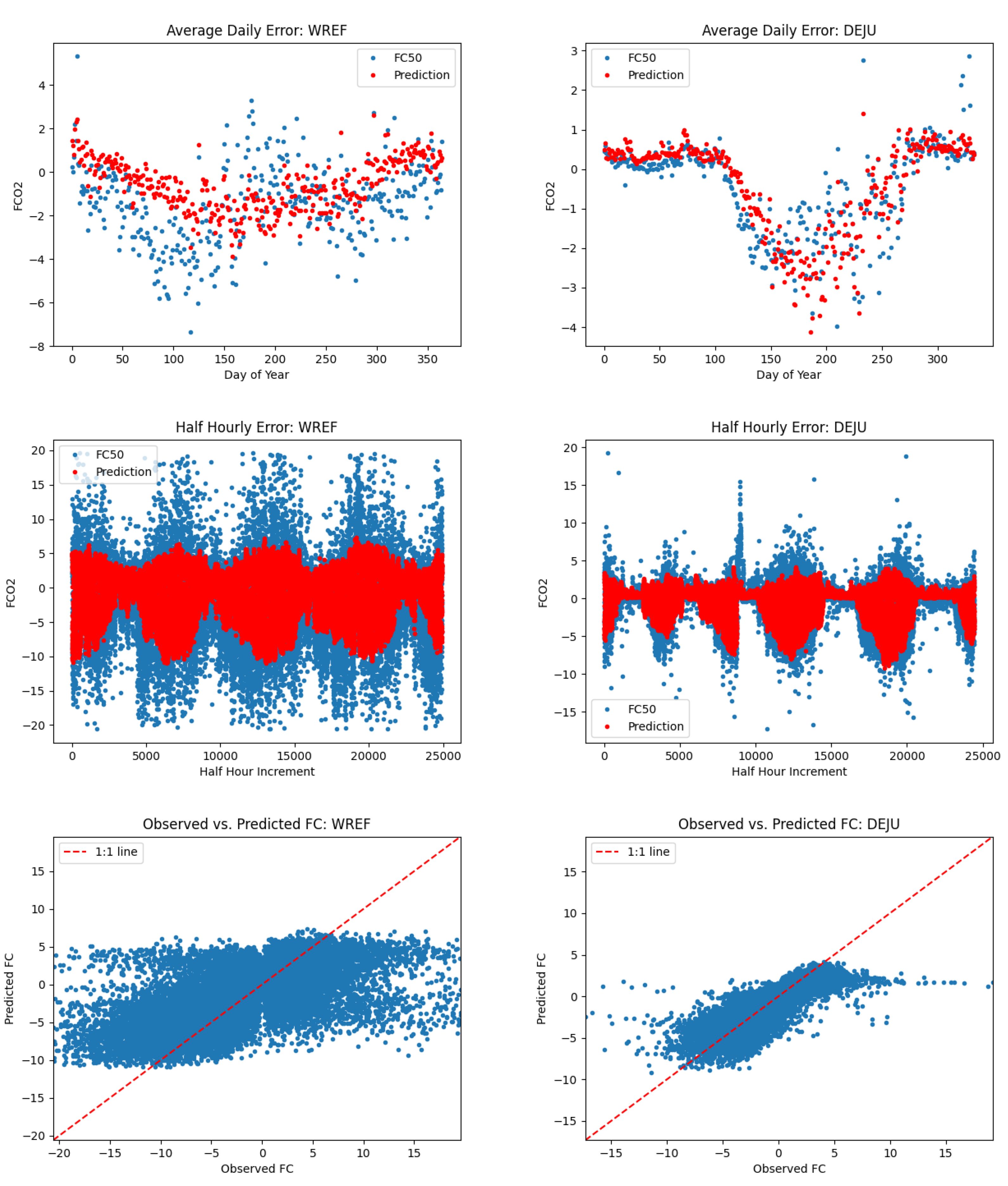

Table 1.
Environmental drivers (feature variables) used as input to our machine learning models to predict carbon dioxide flux
Table 1.
Environmental drivers (feature variables) used as input to our machine learning models to predict carbon dioxide flux
| Variable | Description | Source | Mean | Min | Max |
|---|---|---|---|---|---|
| DOY | Day Of Year | AmeriFlux/NEON | 0.49 | 0 | 1 |
| HOUR | Hour Of Day | AmeriFlux/NEON | 0.49 | 0 | 1 |
| TS_1_1_1 | Soil Temperature Depth 1 | AmeriFlux/NEON | 12.64 | -29.82 | 56.15 |
| TS_1_2_1 | Soil Temperature Depth 2 | AmeriFlux/NEON | 12.17 | -29.85 | 52.52 |
| PPFD | Photosynthetic Photon Flux Density | AmeriFlux/NEON | 563.72 | -2.27 | 2772.22 |
| TAIR | Air Temperature | AmeriFlux/NEON | 12.14 | -36.39 | 41.85 |
| VPD | Vapor Pressure Deficit | AmeriFlux/NEON | 8.48 | -0.57 | 74.49 |
| SWC_1_1_1 | Soil Water Content | AmeriFlux/NEON | 19.74 | 0.25 | 40.96 |
| PPFD_OUT | Photosynthetic Photon Flux Density, Outgoing | AmeriFlux/NEON | 60.92 | -2.29 | 2054.03 |
| PPFD_BC_IN_1_1_1 | Photosynthetic Photon Flux Density, Below Canopy Incoming | AmeriFlux/NEON | 193.89 | -9.44 | 2638.5 |
| RH | Relative Humidity | AmeriFlux/NEON | 57.03 | 1.35 | 101.95 |
| NETRAD | Net Radiation | AmeriFlux/NEON | 152.55 | -308.42 | 1056.68 |
| USTAR | Friction velocity | AmeriFlux/NEON | 0.46 | 0.05 | 2.78 |
| GCC_50 | Green Chromatic Coordinate, 50th Quantile | Phenocam | 0.36 | 0.29 | 0.46 |
| RCC_50 | Red Chromatic Coordinate, 50th Quantile | Phenocam | 0.4 | 0.26 | 0.58 |
| MAT_DAYMET | Mean Annual Temperature | DAYMET | 9.7 | -11.6 | 26.1 |
| MAP_DAYMET | Mean Annual Precipitation | DAYMET | 872.85 | 86 | 2290 |
| PVEG | Primary Vegetation Type | Phenocam | categorical | ||
| SVEG | Secondary Vegetation Type | Phenocam | categorical | ||
| LW_OUT | Longwave Radiation, Outgoing | AmeriFlux/NEON | 378.09 | 165.3 | 694.8 |
| DAILY PRECIPITATION | Daily Precipitation | AmeriFlux/NEON | 2.2 | 0 | 225.19 |
| PRCP1WEEK | Cummulative Precipitation 1 Week | AmeriFlux/NEON | 16.42 | 0 | 262.73 |
| PRCP2WEEK | Cumulative Precipitation 2 Week | AmeriFlux/NEON | 33.59 | 0 | 324.87 |
| NDVI | Normalized Difference Vegetation Index | MODIS | 0.47 | -0.2 | 0.96 |
| EVI | Enhanced Vegetation Index | MODIS | 0.26 | -0.13 | 0.76 |
| LAT | Latitude | Phenocam | 41.19 | 17.97 | 71.28 |
| LON | Longitude | Phenocam | -101.8 | -156.62 | -66.87 |
| ELEV | Elevation | Phenocam | 813.93 | 7 | 3493 |
| DOMAIN | NEON Field Site Domain | Phenocam | categorical | ||
| organic_C | Total Organic Carbon Stock in Soil Profile | AmeriFlux/NEON | 255.87 | 5 | 1339 |
| total_N | Total Nitrogen Stock in Soil Profile | AmeriFlux/NEON | 13.47 | 0.3 | 43.6 |
| O_thickness | Total Thickness of Organic Horizon | AmeriFlux/NEON | 3.49 | 0 | 110 |
| A_pH | pH of A Horizon | AmeriFlux/NEON | 6.03 | 0 | 8.5 |
| A_sand | Texture of A Horizon (% Sand) | AmeriFlux/NEON | 47.78 | 0 | 97 |
| A_silt | Texture of A Horizon (% Silt) | AmeriFlux/NEON | 32.57 | 0 | 61.9 |
| A_clay | Texture of A Horizon (% Clay) | AmeriFlux/NEON | 15.08 | 0 | 55.3 |
| A_BD | Bulk Density of A Horizon | AmeriFlux/NEON | 0.93 | 0 | 1.59 |
Table 2.
Comparison of the RMSE and R2 in predicting FCO2 using seven machine learning models in a 10-fold cross-validation experimental setting (values shown are the average across the 10 validation folds)
Table 2.
Comparison of the RMSE and R2 in predicting FCO2 using seven machine learning models in a 10-fold cross-validation experimental setting (values shown are the average across the 10 validation folds)
| Linear reg | Stepwise | Decision Tree | Random Forest | XGB | NN 1-layer | NN deeper | |
|---|---|---|---|---|---|---|---|
| RMSE | 3.49 | 3.58 | 2.39 | 2.26 | 1.81 | 2.06 | 1.91 |
| R2 | 0.48 | 0.46 | 0.76 | 0.77 | 0.86 | 0.82 | 0.85 |
Table 3.
A comparison of the RMSE (molm−2s−1) in predicting FCO2 using seven machine learning models in a stratified leave-one-site-out cross-validation experimental setting
Table 3.
A comparison of the RMSE (molm−2s−1) in predicting FCO2 using seven machine learning models in a stratified leave-one-site-out cross-validation experimental setting
| Test Set | Site Code | Site Name | Primary Vegtype | Linear reg | Stepwise | Decision Tree | Random Forest | XGB | NN 1-layer | NN deeper |
|---|---|---|---|---|---|---|---|---|---|---|
| 1 | PR-xGU | Guanica Forest (GUAN) | EB | 4.83 | 4.47 | 5.83 | 5.32 | 3.49 | 5.95 | 6.48 |
| 2 | PR-xLA | Lajas Experimental Station (LAJA) | EB | 7.52 | 6.99 | 7.60 | 6.68 | 6.22 | 6.02 | 6.60 |
| 3 | US-xAB | Abby Road (ABBY) | EN | 7.25 | 4.45 | 4.72 | 3.86 | 3.43 | 3.55 | 3.66 |
| 4 | US-xBA | Barrow Environmental Observatory (BARR) | TN | 135.35 | 1.30 | 1.51 | 1.49 | 0.86 | 2.91 | 0.89 |
| 5 | US-xBL | Blandy Experimental Farm (BLAN) | DB | 4.10 | 3.96 | 2.77 | 2.69 | 2.62 | 2.89 | 2.98 |
| 6 | US-xBN | Caribou Creek - Poker Flats Watershed (BONA) | EN | 14.61 | 2.41 | 2.12 | 2.01 | 1.93 | 2.70 | 1.92 |
| 7 | US-xBR | Bartlett Experimental Forest (BART) | DB | 5.21 | 4.41 | 3.33 | 3.06 | 2.77 | 3.13 | 3.06 |
| 8 | US-xCL | LBJ National Grassland (CLBJ) | DB | 5.19 | 4.17 | 4.38 | 4.16 | 3.88 | 4.11 | 3.31 |
| 9 | US-xCP | Central Plains Experimental Range (CPER) | GR | 4.24 | 2.47 | 1.38 | 1.29 | 1.22 | 1.60 | 1.48 |
| 10 | US-xDC | Dakota Coteau Field School (DCFS) | GR | 20.35 | 2.70 | 1.79 | 1.70 | 1.61 | 1.64 | 1.74 |
| 11 | US-xDJ | Delta Junction (DEJU) | EN | 5.52 | 2.28 | 2.05 | 1.64 | 1.44 | 1.56 | 1.44 |
| 12 | US-xDL | Dead Lake (DELA) | DB | 9.86 | 5.29 | 4.36 | 4.21 | 3.84 | 4.23 | 4.26 |
| 13 | US-xDS | Disney Wilderness Preserve (DSNY) | GR | 10.21 | 3.03 | 3.64 | 3.25 | 3.33 | 2.67 | 3.35 |
| 14 | US-xGR | Great Smoky Mountains National Park, Twin Creeks (GRSM) | DB | 6.51 | 6.06 | 4.21 | 3.99 | 3.87 | 4.12 | 3.94 |
| 15 | US-xHA | Harvard Forest (HARV) | DB | 5.24 | 4.50 | 3.05 | 2.91 | 2.60 | 2.73 | 2.92 |
| 16 | US-xHE | Healy (HEAL) | TN | 5.03 | 1.72 | 2.00 | 1.65 | 1.15 | 1.77 | 1.17 |
| 17 | US-xJE | Jones Ecological Research Center (JERC) | DB | 6.07 | 4.37 | 3.75 | 3.46 | 3.19 | 3.43 | 3.41 |
| 18 | US-xJR | Jornada LTER (JORN) | GR | 2.56 | 1.79 | 1.25 | 1.23 | 1.17 | 1.76 | 1.26 |
| 19 | US-xKA | Konza Prairie Biological Station - Relocatable (KONA) | AG | 6.57 | 3.64 | 3.02 | 2.95 | 2.61 | 3.05 | 3.56 |
| 20 | US-xKZ | Konza Prairie Biological Station (KONZ) | GR | 6.88 | 3.57 | 2.60 | 2.23 | 2.21 | 2.06 | 2.16 |
| 21 | US-xLE | Lenoir Landing (LENO) | DB | 6.83 | 5.27 | 4.92 | 4.53 | 4.32 | 4.25 | 4.19 |
| 22 | US-xMB | Moab (MOAB) | GR | 8.63 | 1.86 | 0.73 | 0.71 | 0.68 | 1.54 | 0.68 |
| 23 | US-xNG | Northern Great Plains Research Laboratory (NOGP) | GR | 5.07 | 2.29 | 1.67 | 1.59 | 1.46 | 1.55 | 1.96 |
| 24 | US-xNQ | Onaqui-Ault (ONAQ) | SH | 4.01 | 1.73 | 1.17 | 1.11 | 1.05 | 1.90 | 1.21 |
| 25 | US-xNW | Niwot Ridge Mountain Research Station (NIWO) | TN | 9.63 | 1.46 | 0.85 | 0.80 | 0.74 | 1.86 | 1.76 |
| 26 | US-xRM | Rocky Mountain National Park, CASTNET (RMNP) | EN | 8.49 | 3.18 | 2.70 | 2.31 | 1.92 | 2.45 | 1.94 |
| 27 | US-xRN | Oak Ridge National Lab (ORNL) | DB | 5.75 | 5.11 | 4.43 | 4.22 | 3.68 | 3.92 | 3.61 |
| 28 | US-xSB | Ordway-Swisher Biological Station (OSBS) | EN | 7.77 | 3.40 | 3.06 | 2.78 | 2.63 | 3.17 | 3.08 |
| 29 | US-xSC | Smithsonian Conservation Biology Institute (SCBI) | DB | 4.53 | 4.11 | 3.36 | 3.00 | 2.86 | 3.12 | 2.98 |
| 30 | US-xSE | Smithsonian Environmental Research Center (SERC) | DB | 6.79 | 4.62 | 3.40 | 3.21 | 3.08 | 3.35 | 3.32 |
| 31 | US-xSJ | San Joaquin Experimental Range (SJER) | EN | 5.13 | 4.23 | 3.23 | 3.11 | 3.02 | 3.23 | 3.81 |
| 32 | US-xSL | North Sterling, CO (STER) | AG | 6.10 | 2.40 | 2.00 | 1.93 | 1.83 | 1.90 | 2.08 |
| 33 | US-xSP | Soaproot Saddle (SOAP) | EN | 3.57 | 3.58 | 4.16 | 3.86 | 2.50 | 2.78 | 2.67 |
| 34 | US-xSR | Santa Rita Experimental Range (SRER) | SH | 3.22 | 2.19 | 4.23 | 3.63 | 1.18 | 2.42 | 1.12 |
| 35 | US-xST | Steigerwaldt Land Services (STEI) | DB | 3.96 | 4.06 | 2.44 | 2.10 | 1.91 | 2.34 | 1.78 |
| 36 | US-xTA | Talladega National Forest (TALL) | EN | 5.36 | 5.16 | 4.53 | 4.33 | 3.34 | 3.77 | 3.98 |
| 37 | US-xTE | Lower Teakettle (TEAK) | EN | 6.11 | 3.07 | 2.99 | 2.93 | 2.53 | 2.48 | 2.95 |
| 38 | US-xTL | Toolik (TOOL) | TN | 134.54 | 1.44 | 1.24 | 0.79 | 0.66 | 2.12 | 0.96 |
| 39 | US-xTR | Treehaven (TREE) | DB | 5.13 | 3.89 | 2.41 | 2.35 | 2.12 | 2.61 | 2.21 |
| 40 | US-xUK | The University of Kansas Field Station (UKFS) | DB | 5.16 | 4.12 | 3.20 | 3.06 | 2.92 | 3.56 | 2.92 |
| 41 | US-xUN | University of Notre Dame Environmental Research Center (UNDE) | DB | 3.79 | 3.81 | 2.51 | 2.47 | 2.11 | 2.53 | 1.92 |
| 42 | US-xWD | Woodworth (WOOD) | GR | 5.16 | 2.21 | 1.77 | 1.61 | 1.49 | 1.52 | 1.70 |
| 43 | US-xWR | Wind River Experimental Forest (WREF) | EN | 7.53 | 5.31 | 5.89 | 5.82 | 4.67 | 4.92 | 4.68 |
| 44 | US-xYE | Yellowstone Northern Range (Frog Rock) (YELL) | EN | 5.05 | 2.49 | 2.10 | 2.05 | 1.61 | 1.71 | 1.74 |
| AVERAGE | 12.28 | 3.51 | 3.05 | 2.82 | 2.45 | 2.88 | 2.70 |
Table 4.
A comparison of the R2 in predicting FCO2 using seven machine learning models in a stratified leave-one-site-out cross-validation experimental setting
Table 4.
A comparison of the R2 in predicting FCO2 using seven machine learning models in a stratified leave-one-site-out cross-validation experimental setting
| Test Set | Site Code | Site Name | Primary Vegtype | Linear reg | Stepwise | Decision Tree | Random Forest | XGBoost | NN (1-layer) | NN (deep) |
|---|---|---|---|---|---|---|---|---|---|---|
| 1 | PR-xGU | Guanica Forest (GUAN) | EB | 0.07 | 0.21 | -0.35 | -0.12 | 0.52 | -0.40 | -0.67 |
| 2 | PR-xLA | Lajas Experimental Station (LAJA) | EB | 0.31 | 0.40 | 0.29 | 0.45 | 0.53 | 0.56 | 0.47 |
| 3 | US-xAB | Abby Road (ABBY) | EN | -0.37 | 0.48 | 0.42 | 0.61 | 0.69 | 0.67 | 0.65 |
| 4 | US-xBA | Barrow Environmental Observatory (BARR) | TN | -16320.00 | -0.51 | -1.03 | -0.97 | 0.34 | -6.54 | 0.29 |
| 5 | US-xBL | Blandy Experimental Farm (BLAN) | DB | 0.54 | 0.57 | 0.79 | 0.80 | 0.81 | 0.77 | 0.76 |
| 6 | US-xBN | Caribou Creek - Poker Flats Watershed (BONA) | EN | -33.28 | 0.07 | 0.28 | 0.35 | 0.40 | -0.17 | 0.41 |
| 7 | US-xBR | Bartlett Experimental Forest (BART) | DB | 0.34 | 0.53 | 0.73 | 0.77 | 0.81 | 0.76 | 0.77 |
| 8 | US-xCL | LBJ National Grassland (CLBJ) | DB | 0.35 | 0.58 | 0.54 | 0.58 | 0.64 | 0.59 | 0.74 |
| 9 | US-xCP | Central Plains Experimental Range (CPER) | GR | -4.44 | -0.85 | 0.42 | 0.50 | 0.55 | 0.22 | 0.33 |
| 10 | US-xDC | Dakota Coteau Field School (DCFS) | GR | -28.15 | 0.49 | 0.78 | 0.80 | 0.82 | 0.81 | 0.79 |
| 11 | US-xDJ | Delta Junction (DEJU) | EN | -3.89 | 0.17 | 0.32 | 0.57 | 0.67 | 0.61 | 0.67 |
| 12 | US-xDL | Dead Lake (DELA) | DB | -0.89 | 0.46 | 0.63 | 0.66 | 0.71 | 0.65 | 0.65 |
| 13 | US-xDS | Disney Wilderness Preserve (DSNY) | GR | -3.07 | 0.64 | 0.48 | 0.59 | 0.57 | 0.72 | 0.56 |
| 14 | US-xGR | Great Smoky Mountains National Park, Twin Creeks (GRSM) | DB | 0.39 | 0.48 | 0.75 | 0.77 | 0.79 | 0.76 | 0.78 |
| 15 | US-xHA | Harvard Forest (HARV) | DB | 0.31 | 0.49 | 0.77 | 0.79 | 0.83 | 0.81 | 0.79 |
| 16 | US-xHE | Healy (HEAL) | TN | -4.45 | 0.36 | 0.14 | 0.41 | 0.72 | 0.33 | 0.71 |
| 17 | US-xJE | Jones Ecological Research Center (JERC) | DB | 0.19 | 0.58 | 0.69 | 0.74 | 0.78 | 0.74 | 0.75 |
| 18 | US-xJR | Jornada LTER (JORN) | GR | -2.75 | -0.85 | 0.11 | 0.13 | 0.21 | -0.77 | 0.09 |
| 19 | US-xKA | Konza Prairie Biological Station - Relocatable (KONA) | AG | -1.33 | 0.28 | 0.51 | 0.53 | 0.63 | 0.50 | 0.31 |
| 20 | US-xKZ | Konza Prairie Biological Station (KONZ) | GR | -0.85 | 0.50 | 0.74 | 0.81 | 0.81 | 0.83 | 0.82 |
| 21 | US-xLE | Lenoir Landing (LENO) | DB | 0.19 | 0.52 | 0.58 | 0.64 | 0.67 | 0.69 | 0.69 |
| 22 | US-xMB | Moab (MOAB) | GR | -145.46 | -5.79 | -0.05 | 0.01 | 0.09 | -3.66 | 0.09 |
| 23 | US-xNG | Northern Great Plains Research Laboratory (NOGP) | GR | -2.17 | 0.36 | 0.66 | 0.69 | 0.74 | 0.71 | 0.52 |
| 24 | US-xNQ | Onaqui-Ault (ONAQ) | SH | -7.30 | -0.54 | 0.29 | 0.37 | 0.43 | -0.87 | 0.25 |
| 25 | US-xNW | Niwot Ridge Mountain Research Station (NIWO) | TN | -120.13 | -1.77 | 0.05 | 0.17 | 0.28 | -3.53 | -3.04 |
| 26 | US-xRM | Rocky Mountain National Park, CASTNET (RMNP) | EN | -5.45 | 0.09 | 0.35 | 0.52 | 0.67 | 0.46 | 0.66 |
| 27 | US-xRN | Oak Ridge National Lab (ORNL) | DB | 0.25 | 0.41 | 0.56 | 0.60 | 0.69 | 0.65 | 0.71 |
| 28 | US-xSB | Ordway-Swisher Biological Station (OSBS) | EN | -1.39 | 0.54 | 0.63 | 0.69 | 0.73 | 0.60 | 0.62 |
| 29 | US-xSC | Smithsonian Conservation Biology Institute (SCBI) | DB | 0.42 | 0.52 | 0.68 | 0.74 | 0.77 | 0.72 | 0.75 |
| 30 | US-xSE | Smithsonian Environmental Research Center (SERC) | DB | -0.01 | 0.53 | 0.75 | 0.77 | 0.79 | 0.75 | 0.76 |
| 31 | US-xSJ | San Joaquin Experimental Range (SJER) | EN | -0.51 | -0.03 | 0.40 | 0.44 | 0.47 | 0.40 | 0.17 |
| 32 | US-xSL | North Sterling, CO (STER) | AG | -4.83 | 0.10 | 0.38 | 0.42 | 0.47 | 0.44 | 0.32 |
| 33 | US-xSP | Soaproot Saddle (SOAP) | EN | -0.98 | -0.98 | -1.68 | -1.31 | 0.03 | -0.19 | -0.10 |
| 34 | US-xSR | Santa Rita Experimental Range (SRER) | SH | -7.73 | -3.04 | -14.04 | -10.11 | -0.18 | -3.93 | -0.06 |
| 35 | US-xST | Steigerwaldt Land Services (STEI) | DB | 0.53 | 0.50 | 0.82 | 0.87 | 0.89 | 0.83 | 0.90 |
| 36 | US-xTA | Talladega National Forest (TALL) | EN | 0.39 | 0.44 | 0.57 | 0.60 | 0.76 | 0.70 | 0.66 |
| 37 | US-xTE | Lower Teakettle (TEAK) | EN | -2.27 | 0.17 | 0.22 | 0.25 | 0.44 | 0.46 | 0.24 |
| 38 | US-xTL | Toolik (TOOL) | TN | -12181.30 | -0.40 | -0.03 | 0.58 | 0.71 | -2.01 | 0.38 |
| 39 | US-xTR | Treehaven (TREE) | DB | 0.24 | 0.57 | 0.83 | 0.84 | 0.87 | 0.80 | 0.86 |
| 40 | US-xUK | The University of Kansas Field Station (UKFS) | DB | 0.24 | 0.52 | 0.71 | 0.73 | 0.76 | 0.64 | 0.76 |
| 41 | US-xUN | University of Notre Dame Environmental Research Center (UNDE) | DB | 0.56 | 0.55 | 0.81 | 0.81 | 0.86 | 0.80 | 0.89 |
| 42 | US-xWD | Woodworth (WOOD) | GR | -2.01 | 0.45 | 0.65 | 0.71 | 0.75 | 0.74 | 0.67 |
| 43 | US-xWR | Wind River Experimental Forest (WREF) | EN | -0.65 | 0.18 | -0.01 | 0.02 | 0.37 | 0.30 | 0.36 |
| 44 | US-xYE | Yellowstone Northern Range (Frog Rock) (YELL) | EN | -2.28 | 0.20 | 0.43 | 0.46 | 0.67 | 0.62 | 0.61 |
| AVERAGE | -656.42 | -0.02 | 0.06 | 0.23 | 0.60 | -0.01 | 0.44 |
Table 5.
Table of Mean Bias and Correlation Coefficient (r) using L1SO predicted annual carbon sums and 10-fold projections of annual carbon sums.
Table 5.
Table of Mean Bias and Correlation Coefficient (r) using L1SO predicted annual carbon sums and 10-fold projections of annual carbon sums.
| Primary Vegetation | Site | Mean Bias | R |
|---|---|---|---|
| AG | US-xSL | -15.80 | 0.58 |
| US-xKA | 4.73 | 0.22 | |
| AVERAGE | -5.53 ± 10.27 | 0.40 ± 0.18 | |
| DB | US-xSC | -60.82 | |
| US-xLE | 134.12 | ||
| US-xJE | 76.42 | 0.68 | |
| US-xHA | -46.71 | 0.32 | |
| US-xGR | 20.46 | 0.05 | |
| US-xRN | -67.14 | 0.82 | |
| US-xDL | 55.57 | -0.56 | |
| US-xST | 21.37 | 0.75 | |
| US-xSE | 17.43 | -0.36 | |
| US-xCL | 170.94 | -0.78 | |
| US-xBR | 114.38 | 0.85 | |
| US-xTR | -3.15 | 0.96 | |
| US-xBL | 135.44 | 0.019 | |
| US-xUK | 1.47 | 0.98 | |
| US-xUN | 4.95 | -0.44 | |
| AVERAGE | 38.32 ± 71.72 | 0.25 ± 0.64 | |
| EB | PR-xLA | 140.70 | |
| PR-xGU | 31.93 | ||
| AVERAGE | 86.32 ± 54.38 | ||
| EN | US-xSB | 121.02 | -0.20 |
| US-xSP | -44.92 | 0.48 | |
| US-xTA | -68.90 | 0.32 | |
| US-xTE | 47.40 | -0.35 | |
| US-xSJ | -15.44 | -0.65 | |
| US-xRM | -48.55 | -0.67 | |
| US-xYE | 4.31 | 0.57 | |
| US-xDJ | 20.68 | 0.24 | |
| US-xWR | -10.31 | -0.92 | |
| US-xAB | 52.29 | 0.09 | |
| US-xBN | -18.25 | 0.55 | |
| AVERAGE | 3.57 ± 51.99 | -0.05 ± 0.51 | |
| GR | US-xWD | -5.97 | 0.62 |
| US-xCP | -9.58 | 0.52 | |
| US-xDC | 21.99 | 0.88 | |
| US-xMB | 17.88 | 0.98 | |
| US-xDS | 230.26 | -0.90 | |
| US-xJR | 28.82 | 0.63 | |
| US-xKZ | 19.34 | -0.62 | |
| US-xNG | 34.74 | 0.85 | |
| AVERAGE | 42.18 ± 72.57 | 0.37 ± 0.67 | |
| SH | US-xSR | -61.37 | 0.99 |
| US-xNQ | 63.5 | 0.99 | |
| AVERAGE | 1.07 ± 62.44 | 0.99 ± 0.01 | |
| TN | US-xNW | -28.12 | 0.95 |
| US-xHE | -12.39 | 0.76 | |
| US-xTL | -22.12 | 0.54 | |
| US-xBA | -29.72 | 0.81 | |
| AVERAGE | -23.09 ± 6.80 | 0.77 ± 0.15 |
Disclaimer/Publisher’s Note: The statements, opinions and data contained in all publications are solely those of the individual author(s) and contributor(s) and not of MDPI and/or the editor(s). MDPI and/or the editor(s) disclaim responsibility for any injury to people or property resulting from any ideas, methods, instructions or products referred to in the content. |
© 2024 by the authors. Licensee MDPI, Basel, Switzerland. This article is an open access article distributed under the terms and conditions of the Creative Commons Attribution (CC BY) license (http://creativecommons.org/licenses/by/4.0/).
Copyright: This open access article is published under a Creative Commons CC BY 4.0 license, which permit the free download, distribution, and reuse, provided that the author and preprint are cited in any reuse.


