
Submitted:
11 December 2024
Posted:
12 December 2024
You are already at the latest version
Abstract
In this paper, the method to determine the percentiles of the P-S-N field when it presents bilinear (s1 and s2) behavior (e.g competence failure mode) is given. The percentiles are determined around the Weibull scale (η) parameter in Cycles that corresponds to the median applied stress of the whole bilinear behavior. The reliability (R(t)) index that corresponds to each P-S-N percentile are also determined. As well as the confidence reliability percentile (CL) that corresponds to each P-S-N percentile. The formulation to relate CL with its corresponding normal P-S-N percentile is also given. Numerically, the percentiles of the normal (one, two, and three) sigma levels, as well as those that correspond to the capability Cp and Cpk indices are related with their CL values, and R(t) indices. To validate the Weibull cycle bilinear family, a test plan is designed and numerically performed. In the numerical application we use the 42CrMo4 steel material.
Keywords:
fatigue P-S-N field
; Weibull/IPL model
; bilinear model
; reliability percentiles
; testing plan
; capability indices
; six sigma
1. Introduction
Fatigue is one of the principal causes of failure in mechanical and structural elements [1]. When the fatigue element presents different fatigue slopes, determining from both behaviors an equivalent S-N slope is fundamental. Then the equivalent slope is used on the Basquin model to characterize the bilinear fatigue behavior as in ASTM 739 standard [2] and Eurocode 3 [3]. However, the Basquin model is efficient only for linear behavior. Thus, because the Basquin model does not represent multiple failure modes, its use is not efficient to represent the bilinear behavior [4]. In a S-N curve a bilinear behavior represents a transition between two competitive failure modes, or a step of variant stress. In the fatigue frame this transition is called a knee-point [5]. And although its consideration improves the analysis, it does not incorporate the probabilistic behavior [6]. Thus, because fatigue is random, formulating a probabilistic P-S-N curve method is necessary to get a more reliable failure prediction [7].
During the last decades, several fatigue probabilistic models have been proposed. Castillo and Canteli [8] introduced the Weibull fatigue model. In [9], a model for fatigue crack growth was formulated. In [10], a model for fatigue based on the statistical characteristics of the cycles to failure was given. Similar research is found in [11]. Unfortunately, none of them are focused on bilinear behavior. Among research focused on bilinear behavior we have [12]. They mention that to improve fatigue life prediction, a bilinear model with probabilistic focus must be used to model the uncertainties associated with the deterioration process produced by fatigue phenomenon. In [13], an application of the bilinear model to fourteen kinds of alloys was performed. They show that this model provides a better representation of fatigue behavior than the linear model. However, despite their utility, both linear and bilinear models lack probabilistic information.
Therefore, the novelty of this paper is the method to consider the probabilistic behavior in the bilinear fatigue analysis and to generate its corresponding P-S-N field (see Table 8). The used material for the analysis is 42CrMo4 steel. And since the material S-N curve represents median values, then the analysis was performed based on the median stress of collected data (see Table 1). And because the reliability index is based on the time domain then the Weibull parameters in cycles to failure that corresponds to the median stress value were determined. They are . Consequently, by considering to be constant, the P-S-N percentiles were determined around . However, because for each estimated percentile, its corresponding eta () value exists, and since for each value different index is determined, then the confidence reliability percentile () that corresponds to the difference between the value and cycles were also determined. Additionally, the formulation to relate the value with the P-S-N percentile was also given. Therefore, a summary table that shows the P-S-N percentile, the value, the index and the minimum and maximum values is presented for the one, two, and three sigma levels, as well as those that correspond to the capability and indices. Finally, the test plan that can be used to validate the Weibull cycle bilinear family is designed and numerically performed to show how the proposed methodology can be implemented.
2. Bilinear and Weibull/IPL General Background
In fatigue analysis, it is fundamental to understand the models for evaluating the service life of materials. This section offers the fundamentals of the fatigue models, emphasizing the S-N curve and the Basquin equation. We also discussed the bilinear model for fatigue characterization and present the Weibull distribution and the Weibull/IPL model concepts which play a key role in the P-S-N analysis.
2.1. Fatigue Model
When mechanical elements are subject to cycling loading, a fatigue analysis is required. The analysis requires determining the cycles until the material fails. Its graphical representation is the S-N curve, also known Wöhler curve, where the stress () is plotted against the logarithm of the cycles to failure () [14]. The relationship between applied stress and the number of cycles is given by the Basquin model:
Where is the slope and is the ordinate to the origin. Its application to the bilinear behavior is as follows.
2.2. Bilinear Model
The bilinear model is an extension of the linear model used in fatigue analysis. In the bilinear behavior, the S-N curve of a material is divided into two regions, because of the change of the slope. For example, region I can be governed by the plastic region, while Region II can be governed by the elastic zone. The point where the two regions intersect is called knee-point [5]. The S-N curve shown in Figure 1, is characterized by a high slope in the first phase of the bilinear model, and a low slope in the second phase.
Understanding the characteristics of the S-N curve, particularly the knee-point is crucial for fatigue analysis. The high slope in the first phase indicates a higher rate of damage accumulation, whereas the second phase, with its lower slope, suggests a slower progression of fatigue. Thus, to consider the spread of data, a probability function is necessary. Here we use the Weibull distribution. Its generalities are as follows.
2.3. Weibull Distribution
The Weibull distribution is widely used in reliability analysis [15]. It was proposed by Wallody Weibull [16], and its probability density function (pdf) is given by:
The corresponding reliability and cumulative failure distribution are:
Where is the shape parameter and is the scale parameter. Furthermore, the Inverse Power Law (IPL) model, which is frequently used to relate the failure times with a non-thermal stresses [17], is defined by:
Where represents characteristic life, represents the stress level, and and are parameters to be determined. By setting in eq.(2), the Weibull/IPL model is as follows:
Thus, the Weibull/IPL reliability function is given by:
The parameters (, , and ) of the Weibull/IPL model defined in eq.(6) are estimated by using the maximum likelihood method. With these Weibull/IPL parameters the steps to perform the P-S-N analysis are as follows.
3. Steps of the Proposed Method
In this section we present the methodological steps to determine the probabilistic P-S-N field. They are:
Step 0. Collect Experimental fatigue data. Collected data must contain failure times and their corresponding stress.
Step 1. Separate data into two homogeneous sets and .
Step 2. Determine the set of data that presents the best fit between times and stress: For each set, determine the multiple regression coefficient , and select the data set with the highest value as the one on which the P-S-N analysis will be performed.
Step 3. For each data set, determine the Weibull/IPL parameters (, , and ) defined in eq.(6).
Step 4. Determine the values that correspond to each stress value of the set and by using its corresponding , , and parameters in eq.(5).
Step 5. For both sets, determine the reliability index that corresponds to each observed failure time using the values of step 4 in eq.(7).
Step 6. Using the , , and parameters of , determine the equivalent failure times of set one (say ) that corresponds to the same reliability percentile () in set two (say ). They are given by:
Step 7. Form the whole set data for the analysis of the P-S-N field by adding to set the equivalent failure times determined in step 6, ( is the set with the highest index).
Step 8. Determine the median stress of the whole stress data.
Step 9. Determine the value in cycles that correspond to the median stress by using the median stress value in eq.(5) with the Weibull/IPL parameters of set .
Step 10. Based on the reliability indices calculated in step 5 and using eq.(8) determine the predicted failure times. Then using the maximum likelihood method determine the Weibull parameters and the Fisher matrix, and using eq.(9) determine the standard deviation of the eta parameter as:
Step 11. Use eqs.(10 and 11) to determine the upper and lower limits of that correspond to a desired P-S-N percentile.
Where is the value of the normal distribution that corresponds to the desired two sizes percentile determined as:
Which for one-sided bound is given as:
Where is the corresponding confidence level. The numerical application is as follows.
4. Numerical Application
In this section the steps to determine the P-S-N field of fatigue data with bilinear behavior and its corresponding testing plan are presented. The bilinear analysis is as follows.
4.1. Bilinear Numerical Analysis
The application is performed by using the 42CrMo4 steel material. Its mechanical properties are Modulus of elasticity; GPa, Poisson ratio , and shear modulus 8GPa. The numerical application aims to demonstrate how the methodology allows us to determine the P-S-N field of 42CrMo4 steel. The methodological steps to perform the bilinear analysis are as follows.
Step 1. The two bilinear behavior groups (First eight data), and (last eleven data) are in Table 1. This data was published in [18].

Table 1.
Fatigue test of 42CrMo4 steel.
| Cycles (N) | 248 | 260 | 280 | 300 | 750 | 770 | 1050 | 1270 | 5000 | 7700 | 7950 | 17200 | 18400 | 27900 | 81000 | 90000 | 152000 | 195000 | 290000 |
| Stress (S) MPa |
890.4 | 947.5 | 934.8 | 933.7 | 822.8 | 790.6 | 793.1 | 796.6 | 679.2 | 665.3 | 668.8 | 649.6 | 637.3 | 639.5 | 595.7 | 595.7 | 586.4 | 553.3 | 558.7 |
Step 2. Because the index for is 0.8083, and for is 0.8280, we select the set as the base set to perform the P-S-N analysis.
Step 3. From eq.(6), by using the maximum likelihood method, the estimated parameters of the Weibull/IPL model for each data set are given in Table 2.
Step 4. By using the (, , and ) parameters of step 3 in eq.(5), the values that correspond to each stress value of Table 1, are given in Table 3:
Step 5. By using the values of Table 3 in eq.(3), The reliability indices of the failure times of both data sets are given in Table 4.
Step 6. The equivalent failure cycles of that should be incorporated to the sets are given in Table 5.
Step 7. The whole set of data that incorporate the equivalent failure times of step 6 into set are given in Table 6.
Step 8. The median stress of the whole set is MPa.
Step 9. From eq.(5), The value that corresponds to the median stress value in cycles is cycles .
Step 10. Using the reliability indices from Table 4 in eq.(3), the predicted failure times are given in Table 7.
By using the maximum likelihood method and the predicted data, the estimated Weibull parameters are , cycles, and from the corresponding Fisher matrix given as:
The standard deviation of is cycles.
Step 11. With cycles in eqs.(9 and 10), the upper and lower limits of its P-S-N field are given in Table 8.
Table 8.
Upper and lower limits of η for severals percentiles.
| Percentile | 50% | 55% | 1σ | 80% | 90% | 95% | 2σ | 97% | 99% | 3σ |
|---|---|---|---|---|---|---|---|---|---|---|
| ηL | 1445.7208 | 1437.8689 | 1411.6007 | 1393.9324 | 1367.6036 | 1346.2362 | 1327.9943 | 1332.5387 | 1307.0509 | 1257.0788 |
| ηU | 1445.7208 | 1453.6180 | 1480.6681 | 1499.4358 | 1528.3025 | 1552.5597 | 1573.8863 | 1568.5189 | 1599.1054 | 1662.6740 |
The percentiles given in Table 8 represent the P-S-N field around the value ( cycles) that corresponds to the analyzed median stress ( MPa). Here we use the median stress because the S-N curve represents median values, but any other desired stress value can be used. Therefore, the Weibull distribution that represents the median stress of the bilinear behavior in cycles is , and its field percentiles are those given in Table 8. Now, the testing plan that we can use to determine the reliability index that the addressed Weibull distribution represents is as follows.
4.2. Test Plan of the Addressed Weibull Distribution
Here we numerically perform the vibration test plan given in appendix C of the GMW3172 norm. The steps to perform the mentioned test plan for the addressed bilinear Weibull distribution are as follows.
Step 1. Determine the six test plan elements. They are 1) Required reliability . 2) Required confidence level for the desired index. 3) The sample size to be tested. 4) The testing time . 5) The Weibull ( and ) parameters. And 6) The testing conditions.
Step 2. Determine the required sample size that corresponds to the addressed value. Based on Piña-Monarrez [19], it is given by:
Step 3. Determine the required testing time. It is the time that corresponds to the desired reliability index. From [20], based on the value of eq.(14) and the bilinear Weibull parameters of step 1, it is given by:
Step 4. Determine the value that corresponds to the required and indices of step 1 as:
Step 5. By using the value, determine the corresponding upper Weibull eta parameter as:
Step 7. By using the testing time of step 3 and from step 5, determine the corresponding reliability index.
Step 8. Determine the P-S-N percentile that corresponds to the required value of step 1 as.
Where was determined in eq.(9). The numerical application is presented as follows.
4.3. Numerical Application of the Test Plan
Step 1, 2 and 3. The required test elements are, , . ( and cycles), . and cycles.
Step 4. The required simple with is 45.5131.
Step 5. Using 45.5131 in eq.(17), the upper bound of the Weibull parameter is cycles.
Step 6. The lower bound of the Weibull parameter cycles.
Step 7. The reliability index corresponding to is .
Step 8. The selected percentiles mentioned in section 1 were determined using in eqs.(17 and 18). Results are given in Table 9.
Based on the designed test plan, it must be performed with a confidence level and a reliability . We must run 46 pieces for a testing time of cycles each, and if none of them fail, we conclude that the analyzed element has a minimum reliability of . However, as observed in Table 9, since is greater than , the expected reliability is . The general conclusions are as follows.
5. Conclusions
1. In practice the bilinear behavior is mainly generated by two competitive failure modes. Although here we are focused on the bilinear behavior of the S-N curve, any bilinear behavior can be analyzed by using the proposed methodology.
2. By applying the methodology, the bilinear behavior can be represented by a Weibull family fitted for a desired stress value. Here because the focus is on the S-N curve, which represents median stresses, we select the median observed stress as the basis of the analysis, but any desired stress value can be used. The median stress value is MPa.
3. The percentiles estimation was performed on the Weibull scale parameter that represents the selected median stress, because we are interested in the reliability index of the analyzed behavior. Notice the shape parameter remains constant. In cycles the addressed Weibull parameters are , Cycles.
4. In general, the P-S-N field of the analysis is given in Table 8, and the percentiles of practical interest are given in Table 9.
5. In the performed test plan of section 4.2., notice the R(t) and CL indices, both determine the required sample size , and in eq.(17) completely determines the upper eta value. And because for any (), , then a confidence interval always exists, implying in any plan test analysis the given methodology can be used.
6. From the test plan data given in the last row of Table 9, notice although the desired reliability was 0.97, because the final reliability is 0.9783. Also notice by the normal and Weibull relationship given in eq.(19) the normal failure percentile that corresponds to is 0.0880.
7. It is very important to notice because the normal and Weibull percentiles defined in eq.(19), depend on the Weibull β value (see eqs.(15 and 17)) then an accurate estimation of β is critical in the analysis. Thus, because in step 10 of sec.3 we determine the β value that represents the bilinear behavior, the proposed methodology is efficient and dynamic to be used in the analysis.
8. As a future research, we recommend determining the sensitive behavior of addressed Weibull family to more accurately determine the expected behavior of β and the variance of η.
Author Contributions
Conceptualization, O.M.-Q, M.R.P.-M. and M.M.H.-R.; methodology, O.M.-Q., M.R.P.-M. and J.F.O.-Y.; formal analysis, O.M.-Q., M.R.P.-M. and J.F.O.-Y.; writing—original draft preparation, O.M.-Q. and M.R.P.-M.; writing—review and editing, O.M.-Q., M.R.P.-M. and M.M.H.-R; supervision, M.R.P.-M.; funding acquisition, M.M.H.-R.; All authors have read and agreed to the published version of the manuscript.
Funding
This research received no external funding.
Institutional Review Board Statement
Not applicable.
Informed Consent Statement
Not applicable.
Data Availability Statement
Not applicable.
Acknowledgments
We appreciate the support of Conahcyt and the Autonomous University of Ciudad Juárez (UACJ) provided in this research.
Conflicts of Interest
The authors declare no conflicts of interest.
References
- Zhang, L. Prediction Method of Fatigue Crack Growth Life of High-Strength Steel for Industry 4.0. 0. IETE J Res. 2022. [CrossRef]
- ASTM standard E-739-91. Standard practice for statistical analysis of linear or linearized stress-life (S-N) and strain-life (ε-N) fatigue data. 2023.
- EN 1993-1-9. Eurocode 3: Design of steel structures - Part 1-9: Fatigue. 2005.
- Wang, M.; Liu, X.; Wang, X.; Wang, Y. Probabilistic modeling of unified S-N curves for mechanical parts. International Journal of Damage Mechanics 2018, 27, 979–999. [Google Scholar] [CrossRef]
- Fatemi, A.; Plaseied, A.; Khosrovaneh, A.K.; Tanner, D. Application of bi-linear log-log S-N model to strain-controlled fatigue data of aluminum alloys and its effect on life predictions. Int J Fatigue 2005, 27, 1040–1050. [Google Scholar] [CrossRef]
- D’Angelo, L.; Nussbaumer, A. Estimation of fatigue S-N curves of welded joints using advanced probabilistic approach. Int J Fatigue 2017, 97, 98–113. [Google Scholar] [CrossRef]
- Villa-Covarrubias, B.; Piña-Monarrez, M.R.; Barraza-Contreras, J.M.; Baro-Tijerina, M. Stress-based weibull method to select a ball bearing and determine its actual reliability. Applied Sciences (Switzerland) 2020, 10, 1–15. [Google Scholar] [CrossRef]
- Castillo, E.; Canteli, A.F. A Unified Statistical Methodology for Modeling Fatigue Damage. 2009. [Google Scholar]
- Wang, T.; Bahrami, Z.; Renaud, G.; Yang, C.; Liao, M.; Liu, Z. A probabilistic model for fatigue crack growth prediction based on closed-form solution. Structures 2022, 44, 1583–1596. [Google Scholar] [CrossRef]
- Xiang, G.; Bacharoudis, K.C.; Vassilopoulos, A.P. Probabilistic fatigue model for composites based on the statistical characteristics of the cycles to failure. Int J Fatigue 2022, 163. [Google Scholar] [CrossRef]
- Mohabeddine, A.; Correia, J.; Montenegro, P.A.; De Jesus, A.; Castro, J.M.; Berto, F. Probabilistic S-N curves for CFRP retrofitted steel details. Int J Fatigue 2021, 148. [Google Scholar] [CrossRef]
- Kwon, K.; Frangopol, D.M.; Soliman, M. Probabilistic Fatigue Life Estimation of Steel Bridges by Using a Bilinear S-N Approach. Journal of Bridge Engineering 2012, 17, 58–70. [Google Scholar] [CrossRef]
- Fatemi, A.; Plaseied, A.; Khosrovaneh, A.K.; Tanner, D. Application of bi-linear log-log S-N model to strain-controlled fatigue data of aluminum alloys and its effect on life predictions. Int J Fatigue 2005, 27, 1040–1050. [Google Scholar] [CrossRef]
- Lorén, S.; Lundström, M. Modelling curved S-N curves. Fatigue Fract Eng Mater Struct 2005, 28, 437–443. [Google Scholar] [CrossRef]
- Zhu, T. Reliability estimation for two-parameter Weibull distribution under block censoring.
- Weibull, W. A Statistical Theory of Strength of Materials. 1939. [Google Scholar]
- Inverse Power Law Relationship. [Online]. Available online: https://help.reliasoft.com/reference/accelerated_life_testing_data_analysis/alt/inverse_power_law_relationship.html (accessed on 25 November 2024).
- Boller, C.; Seeger, T. , Materials data for cyclic loading. Part B, Low Allow steels. 1987; Volume 42. [Google Scholar]
- Piña-Monarrez, M.R. Weibull stress distribution for static mechanical stress and its stress/strength analysis. Qual Reliab Eng Int 2018, 34, 229–244. [Google Scholar] [CrossRef]
- Piña-Monarrez, M.R. Weibull analysis for normal/accelerated and fatigue random vibration test. Qual Reliab Eng Int 2019, 35, 2408–2428. [Google Scholar] [CrossRef]
Figure 1.
S-N curve with bilinear behavior.
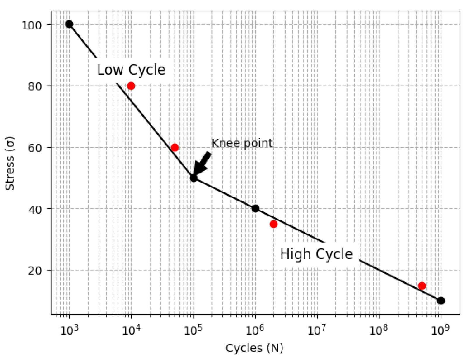
Figure 2.
S-N curve of 42CrMo4.
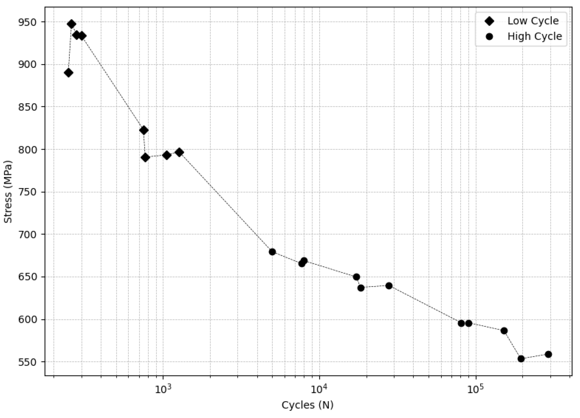
Table 2.
Weibull/IPL parameters for data sets are.
| 6.2428 | 4.74E-28 | 8.3738 | |
| 4.8032 | 3.43E-61 | 20.0032 |
Table 3.
values in MPa for each stress.
| ηi | 29.11 | 8.40 | 11 | 11.26 | 141.24 | 313.88 | 294.67 | 269.83 | 6548.75 | 9903.54 | 8916.79 | 15968.12 | 23405.74 | 21846.65 | 90311.39 | 90311.39 | 123719.22 | 395533.92 | 325694.34 |
| Stress (S) MPa |
890.4 | 947.5 | 934.8 | 933.7 | 822.8 | 790.6 | 793.1 | 796.6 | 679.2 | 665.3 | 668.8 | 649.6 | 637.3 | 639.5 | 595.7 | 595.7 | 586.4 | 553.3 | 558.7 |
Table 4.
Reliability of each failure times.
| Cycles (N) | 248 | 260 | 280 | 300 | 750 | 770 | 1050 | 1270 | 5000 | 7700 | 7950 | 17200 | 18400 | 27900 | 81000 | 90000 | 152000 | 195000 | 290000 |
| R(t) | 0.9643 | 0.2838 | 0.3724 | 0.2396 | 0.5560 | 0.9177 | 0.4957 | 0.0552 | 0.7606 | 0.7419 | 0.5620 | 0.2396 | 0.7299 | 0.0393 | 0.5527 | 0.3740 | 0.0680 | 0.9671 | 0.5640 |
Table 5.
Equivalent Failure Times to use in .
| R(t) | 0.9643 | 0.2838 | 0.3724 | 0.2396 | 0.5560 | 0.9177 | 0.4957 | 0.0552 |
| Neq | 14.60 | 8.81 | 10.97 | 12.13 | 126.41 | 188.26 | 273.73 | 336.71 |
Table 6.
Grouped and data set.
| Ngrouped | 14.60 | 8.81 | 10.97 | 12.13 | 126.41 | 188.26 | 273.73 | 336.71 | 5000 | 7700 | 7950 | 17200 | 18400 | 27900 | 81000 | 90000 | 152000 | 195000 | 290000 |
| Stress (S) |
890.4 | 947.5 | 934.8 | 933.7 | 822.8 | 790.6 | 793.1 | 796.6 | 679.2 | 665.3 | 668.8 | 649.6 | 637.3 | 639.5 | 595.7 | 595.7 | 586.4 | 553.3 | 558.7 |
Table 7.
The predicted Failure Times.
| Npre | 725.206 | 1516.815 | 1442.048 | 1557.252 | 1293.946 | 867.110 | 1342.984 | 1804.107 | 1103.814 | 1124.048 | 1288.972 | 1557.254 | 1136.528 | 1846.307 | 1296.663 | 1440.737 | 1776.197 | 712.747 | 1287.278 |
| R(t) | 0.9643 | 0.2838 | 0.3724 | 0.2396 | 0.5560 | 0.9177 | 0.4957 | 0.0552 | 0.7606 | 0.7419 | 0.5620 | 0.2396 | 0.7299 | 0.0393 | 0.5527 | 0.3740 | 0.0680 | 0.9671 | 0.5640 |
Table 9.
Results of the test plan.
| Percentile | ηU | ηL | CL | R(t) | ||
|---|---|---|---|---|---|---|
| 1σ | 0.6827 | 0.4752623 | 1480.6669 | 1411.5996 | 0.6742 | 0.9732 |
| Cpk | 0.9082 | 1.3297520 | 1545.6359 | 1352.2646 | 0.7480 | 0.9781 |
| Cp | 0.9525 | 1.6695926 | 1572.2603 | 1329.3656 | 0.7761 | 0.9798 |
| 2σ | 0.9545 | 1.6901461 | 1573.8852 | 1327.9932 | 0.7777 | 0.9799 |
| 3σ | 0.9973 | 2.7821505 | 1662.6728 | 1257.0776 | 0.8588 | 0.9846 |
| Test plan | 0.0880 | -1.3531742 | 1547.4550 | 1350.6750 | 0.7500 | 0.9783 |
Disclaimer/Publisher’s Note: The statements, opinions and data contained in all publications are solely those of the individual author(s) and contributor(s) and not of MDPI and/or the editor(s). MDPI and/or the editor(s) disclaim responsibility for any injury to people or property resulting from any ideas, methods, instructions or products referred to in the content. |
© 2024 by the authors. Licensee MDPI, Basel, Switzerland. This article is an open access article distributed under the terms and conditions of the Creative Commons Attribution (CC BY) license (http://creativecommons.org/licenses/by/4.0/).
Copyright: This open access article is published under a Creative Commons CC BY 4.0 license, which permit the free download, distribution, and reuse, provided that the author and preprint are cited in any reuse.


