
Submitted:
09 December 2024
Posted:
10 December 2024
You are already at the latest version
Abstract
The image quality index for whole-body bone scintigraphy has traditionally relied on the total count (Total-C) with a threshold of ≥1.5 mc. However, Total-C measurements are susceptible to variability owing to urine retention. This study aimed to develop a skeletal count (Skel-C)-based index, focusing exclusively on bone regions, to improve the accuracy of image analysis in bone scintigraphy. All cases included herein were Total-C≥1.5 mc. Thresholds were set for Skel-C (0.9–1.2 mc) and Total-C (1.75–2.25 mc); patients were grouped according to whether they were above or below these thresholds. The group including all cases was defined as the Total-C 1.5 high group. Sensitivity and specificity were calculated for each group, and receiver operating characteristic analyses and statistical evaluations were conducted. The specificity of the Skel-C < 0.9 mc group was significantly lower than that of the Skel-C ≥ 0.9 mc group and the Total-C 1.5 high group. These findings highlight the importance of achieving Skel-C ≥ 0.9 mc and suggest that Total-C alone is insufficient for reliable image assessment.
Keywords:
bone scintigraphy
; imaging-analysis program
; skeletal count
; image quality index
; whole-body imaging
1. Introduction
Bone scintigraphy is one of the most frequently performed tests in the field of nuclear medicine [1]. This diagnostic method visualizes the uptake of radiopharmaceuticals into bone [2], aiding in the detection of bone metastases from malignant tumors and the assessment of bone metastasis treatment efficacy [3,4]. Among malignant tumors, prostate cancer frequently presents with osteoblastic bone metastases [5,6], highlighting the critical role of early bone metastasis diagnosis in optimizing treatment decisions [7]. The 2016 Prostate Cancer Practice Guidelines underscore the continued use of bone scintigraphy with 99mTc as the standard technique for diagnosing bone metastases [8]. Additionally, bone scintigraphy is used to estimate prognosis following bone metastasis treatment [9,10]. Typically, the diagnosis through bone scintigraphy relies on visual assessments by a doctor, and the accuracy of these readings can vary based on the examiner's skill and experience, leading to inter-observer variability [11]. BONENAVI (PDR Pharma Co., Ltd.) is an imaging-analysis program for bone scintigraphy designed to assist in image interpretation by automatically identifying high-accumulation areas. This program calculates the skeletal count (Skel-C) by analyzing anterior and posterior bone-scintigraphy images. Importantly, Skel-C focuses solely on the bones, excluding other structures such as the kidneys, bladder, soft tissues, and the peripheral bones of the extremities. The region considered for Skel-C calculation is outlined by solid lines, as depicted in Figure 1.
BONENAVI can obtain two types of counts: Skel-C, which represents the skeletal count, and Total-C, which includes all counts within the imaging field of view. BONENAVI is based on artificial neural networks (ANN) and can assess the likelihood of bone metastases [12], thereby reducing interobserver variability [13]. The ANN-generated value can aid in diagnosis, and its analytical results may influence staging evaluations and subsequent treatment plans. Therefore, BONENAVI serves as a significant diagnostic tool, with numerous studies focusing on enhancing its functionality [14,15,16]. The European Association of Nuclear Medicine guidelines recommend a Total-C of 1.5 million counts (mc) or more for bone scintigraphy [17]. According to Anand et al., the bone scan index (BSI) decreases when Total-C falls below 1 mc; they concluded that, for whole-body bone scintigraphy, the scan speed should be chosen such that Total-C is above 1.5 mc [18]. However, the previous study was based on simulations, and actual Total-C measurements may vary owing to factors such as urine retention and soft-tissue accumulation. We believe that the image count of interest in the image-analysis program is Skel-C, and that Total-C may not contribute directly. Therefore, we hypothesize that the accuracy of the image-analysis program is primarily influenced by Skel-C, rather than by Total-C, which can vary owing to various factors. However, Skel-C is not currently recommended by existing guidelines; to our knowledge, no prior studies have evaluated its use. Thus, this study aimed to develop a new image quality index (Skel-C) to improve the accuracy of bone-scintigraphy imaging-analysis programs.
2. Materials and Methods
2.1. Target Cases
This study included patients who underwent bone scintigraphy between January 2020 and March 2022 due to a suspicion of bone metastases from prostate cancer or for monitoring known bone metastases. The presence of bone metastases was determined by the clinician, and only patients with a Total-C greater than 1.5 mc were included in the study. The study cohort comprised 236 male patients (mean age: 75.1 ± 7.8 [52-91] years; 52-91 years), of whom 81 had bone metastases and 155 did not. This retrospective study was approved by our institutional review board (approval number: 3779) and was conducted in accordance with the ethical standards of the Declaration of Helsinki. The requirement for informed consent was waived.
2.2. Equipment and Analysis Software
The single-photon emission computed tomography/computed tomography (SPECT/CT) systems used in this study were the Discovery NM/CT 670 (GE Healthcare, Chicago, IL, USA) and Bright View X with XCT (Philips Medical Systems International, Cleveland, OH, USA), both equipped with low-energy high-resolution collimators. The nuclear medicine workstations included GENIE-Xeleris (GE Healthcare, Chicago, IL, USA) and Extended Brilliance Workspace Nuclear Medicine (Philips Medical Systems International, Cleveland, OH, USA). The bone-scintigraphy imaging-analysis program BONENAVI® version 2.1.7 (PDRadiopharma Inc., Japan) was employed for image analysis; JMP®16 (SAS Institute, State of North Carolina, USA) and R (The R Foundation for Statistical Computing, Vienna, Austria) [19] were used for statistical data analysis.
2.3. Imaging and Case Grouping
Bone scintigraphy was performed approximately 3–5 h after the patient received an intravenous injection of approximately 740 MBq of 99mTc-methylenediphosphonate (MDP) (PDRadiopharma Inc., Tokyo, Japan). Patients were instructed to urinate immediately before imaging, without the need for aggressive hydration. The imaging parameters were as follows: energy window, 140.5 keV ± 7.5%; pixel size, 2.21 mm; zoom, 1.0; and scanning speed, 12 cm/min. Skel-C thresholds were set at 0.9 mc, 1.0 mc, 1.1 mc, and 1.2 mc, and Total-C thresholds were set at 1.75 mc, 2.0 mc, and 2.25 mc. The groups were defined based on whether Skel-C or Total-C values were below or above the specified thresholds. The group including all cases, regardless of thresholds, was referred to as the Total-C 1.5 high group. Details of each group are presented in Table 1.
2.4. Criteria for the Presence or Absence of Bone Metastasis
The clinician made the final determination regarding the presence or absence of bone metastasis. This judgment was based on a combination of the nuclear medicine specialist’s report, diagnostic imaging findings, laboratory test results, and clinical symptoms.
2.5. Data Analysis
All patients were divided into groups based on the presence or absence of bone metastases. The mean, median, minimum, maximum, and standard deviation (SD) of Total-C and Skel-C were calculated for each group and were assessed for significance using Wilcoxon’s rank-sum test at a 5% significance level. Whole-body images were automatically analyzed using BONENAVI to obtain the ANN values. Based on the criteria for determining the presence of bone metastases, cases with bone metastases confirmed by BONENAVI analysis and an ANN value of 0.5 or higher were defined as true positive cases. Cases with bone metastases that did not meet these criteria were defined as false negative cases. For cases without bone metastases, those with hyper-accumulation regions in the analysis result report and an ANN value of 0.5 or higher were considered false-positive cases. All other cases without bone metastases were classified as true negative cases. The sensitivity and specificity of each group were calculated. Fisher's exact test (significance level: 5%) was performed using JMP Pro®16 to evaluate significant differences between groups. Receiver operating characteristic (ROC) analysis using ANN values was conducted to evaluate the diagnostic performance of each group, and the area under the curve (AUC) was calculated for each group. A bootstrap method (significance level: 5%) was performed using R to evaluate significant differences between groups.
3. Results
All patients were grouped on the basis of the presence or absence of bone metastases. The mean, median, minimum (Min), maximum (Max), and SD of Total-C and Skel-C are summarized in Table 2, with the results of significance tests shown in Figure 2. Skel-C was significantly lower than Total-C in cases with and without bone metastases. Additionally, Skel-C exhibited a lower SD and less variability in counts than Total-C.
Results of the sensitivity and significance tests for each group are presented in Figure 3 and Figure 4. No significant differences were observed in sensitivity values between groups.
The results of specificity for each group and significance tests are presented in Figure 5 and Figure 6. The specificity of the Skel-C 0.9 low group was significantly lower than that of the Skel-C 0.9 high group and the Total-C 1.5 high group. Although not statistically significant, the specificity of the Skel-C 0.9 high, Skel-C 1.0 high, Skel-C 1.1 high, Skel-C 1.2 high, Total-C 1.75 high, Total-C 2.0 high, and Total-C 2.25 high groups exceeded that of the Total-C 1.5 high group.
The results of the AUC and significance tests for each group are presented in Figure 7 and Figure 8. Although no significant differences were found between groups, AUC values of the Skel-C 0.9 high, Skel-C 1.0 high, Skel-C 1.1 high, Skel-C 1.2 high, Total-C 1.75 high, Total-C 2.0 high, and Total-C 2.25 high groups were higher than that of the Total-C 1.5 high group.
4. Discussion
In this study, we focused on developing a new image quality index using the Skel-C index to improve the accuracy of bone-scintigraphy imaging analysis. Total-C and Skel-C were compared to evaluate differences in count variability on whole-body images and the impact of high and low Skel-C and Total-C values on diagnostic performance. As shown in Table 2, the mean, median, and minimum values were higher in the group with bone metastases than in the group without bone metastases. We believe this is because bone metastases typically exhibit stronger radiopharmaceutical accumulation than normal bone. In the Skel-C group, the maximum value was higher in the group without bone metastases. Further, upon examining the case with the maximum value, we found that the patient had a markedly reduced estimated glomerular filtration rate (eGFR = 5). We hypothesize that reduced renal function caused less efflux of radiopharmaceuticals from the body, leading to increased counts. This finding suggests that even in patients without bone metastases, individual physiological differences can cause variations in radiopharmaceutical accumulation in normal bone. The SD of Skel-C was smaller than that of Total-C, regardless of the presence or absence of bone metastases. We attribute this difference to the effects of urinary retention and soft tissue accumulation. Prostate cancer patients often experience dysuria and may have difficulty completely emptying their bladders, even when encouraged to urinate before the examination. Skel-C, which excludes counts from the bladder, soft tissues, and peripheral limb bones, is less affected by these factors. Consequently, we believe that Skel-C reduces variability in whole-body image counts between patients, enhancing the reliability of image quality assessments.
Herein, Skel-C thresholds of 0.9 mc, 1.0 mc, 1.1 mc, and 1.2 mc and Total-C thresholds of 1.75 mc, 2.0 mc, and 2.25 mc were used to classify patients into high and low groups for each threshold, with the aim of identifying the optimal Skel-C threshold. The sensitivity results showed no significant differences between groups divided by Skel-C and Total-C thresholds (Figure 3 and Figure 4). This finding reflects the inherently high sensitivity of bone scintigraphy for detecting bone metastases. False-negative cases primarily included osteolytic bone metastases, small accumulations that were undetectable, and slight residual bone metastases during treatment. Bone scintigraphy is highly sensitive for detecting osteoblastic bone metastases but has lower sensitivity for osteolytic bone metastases [20]. While osteoblastic bone metastases are more common in prostate cancer, osteolytic bone metastases can also occur. In this study, three patients with osteolytic bone metastases were classified as false negatives. The low accumulation of 99mTc-MDP in osteolytic metastases likely contributed to their limited detectability. Additional false-negative cases included three patients with small metastases in the ribs and pelvis and three patients with residual bone metastases alleviated by treatment. Koizumi et al. noted that in patients with small bone metastases or those undergoing treatment, the metastases tend to be smaller, resulting in a lower ANN value and subsequent false-negative results when using analysis software [21]. Since there were no significant differences in sensitivity values among all groups, we conclude that the influence of high and low Total-C and Skel-C values on sensitivity is minimal. Instead, the primary factors influencing sensitivity appear to be the characteristics of individual cases, including the presence of osteolytic metastases, the size of the metastases, and other patient-specific factors. The specificity of the Skel-C 0.9 low group was significantly lower than that of the Skel-C 0.9 high group and the Total-C 1.5 high group. In contrast, no significant differences were observed among groups classified based on Total-C thresholds (Figure 5 and Figure 6). The Total-C 1.5 high group was imaged based on the currently established index, whereas the Skel-C 0.9 low group demonstrated significantly lower specificity. The Skel-C 0.9 low group was also imaged with Total-C values exceeding 1.5 mc; however, its specificity was lower, suggesting that the accuracy of the image-analysis program is more influenced by Skel-C than by Total-C. Because a Total-C-based threshold did not significantly reduce specificity, whereas a Skel-C-based threshold reflected a decrease in specificity, we consider Skel-C to be a valuable image quality index. Although not statistically significant, the Skel-C 0.9 high, Skel-C 1.0 high, Skel-C 1.1 high, Skel-C 1.2 high, Total-C 1.75 high, Total-C 2.0 high, and Total-C 2.25 high groups demonstrated higher specificity and AUC than the Total-C 1.5 high group (Figures 5, 6, 7, and 8). Furthermore, compared to the Total-C 1.5 high group, the Skel-C 0.9 low, Skel-C 1.0 low, Skel-C 1.1 low, and Skel-C 1.2 low groups exhibited lower specificity and AUC. This suggests that including cases with Skel-C < 0.9 mc leads to a decrease in specificity and AUC in the image-analysis program, potentially reducing its diagnostic performance. Since Total-C is influenced by variables such as urine storage and soft tissue accumulation, it may not accurately represent bone uptake. Although Total-C exceeded the recommended threshold of 1.5 mc in all cases, these extraneous factors may reduce its ability to precisely reflect the actual bone count. BONENAVI analyzes bone-scintigraphy images by evaluating the count, location, size, and shape of accumulation sites to generate an ANN value ranging from 0 to 1, which indicates the risk of bone metastasis. A value of 0 represents a negative result, 1 represents a positive result, and 0.5 serves as the threshold for determining the presence of bone metastases [22]. In this study, 31 false-positive cases were reported, and approximately 42% (13 cases) had a Skel-C of less than 0.9 mc. Examples of cases with accumulation in osteophytes classified as true negatives and false positives are illustrated in Figure 9 and Figure 10, respectively.
In Figure 10, Skel-C is low, and the result is a false positive despite the high Total-C. As a feature of the image-analysis program, the whole-body image is subdivided into regions such as the skull, vertebrae, and pelvis. A count threshold is then established based on the counts within these regions, which are recognized as hotspots [22]. Therefore, in cases with low Skel-C, the threshold for recognizing hyperaccumulation sites within each region tends to be lower, likely increasing the likelihood of false positives. In this study, the specificity of Skel-C < 0.9 mc was approximately 64%, which we consider insufficient for the precision required by the imaging-analysis program. In bone scintigraphy, accumulating 99mTc-MDP exclusively in bone metastases is challenging, as it also accumulates in fractures, osteophytes, and osteoarthritis. Improving the ability to differentiate between bone metastases and nonspecific uptake is crucial to enhancing diagnostic accuracy. Low specificity in bone scintigraphy may lead to incorrect identification of bone metastases, potentially resulting in misdiagnosis of prostate cancer staging and affecting subsequent treatment planning [5]. Therefore, a test with both high sensitivity and specificity is essential. Based on the results of this study, we believe that Total-C alone may not accurately reflect the bone area count. Using both Total-C and Skel-C as complementary image quality indexes can improve diagnostic reliability. The specificity of the Skel-C 0.9 low group was significantly lower than that of the Skel-C 0.9 high group and the Total-C 1.5 high group, suggesting that imaging should be conducted with Skel-C values of 0.9 mc or higher. This study highlights the advantages of incorporating Skel-C as an image quality index in bone-scintigraphy imaging-analysis programs.
Factors that may influence Skel-C include the administered dose, post-injection waiting time, and scan speed. Increasing the administered dose is not considered an appropriate approach owing to concerns about increased radiation exposure. Based on the results of this study, we propose an approach to adjust the scan speed and post-injection waiting time to ensure adequate image counts. According to Anand et al. [18], doubling the scan speed reduces the acquired image counts by approximately 50%. Based on this observation, we formulated Equation 1 to determine the optimal scan speed.
Optimal scan speed = Preset scan speed / α
α = 0.9 mc / Lowest Skel-C value observed among the cases (unit: mc)
α = 0.9 mc / Lowest Skel-C value observed among the cases (unit: mc)
In this study, the scan speed was set at 12 cm/min, and the lowest observed Skel-C value was 0.73 mc. To meet the criterion of Skel-C > 0.9 mc, the image count would need to increase by approximately 1.233 times. Using Equation 1, the optimal scan speed was calculated to be approximately 9.73 cm/min. However, extending the scan time increases the risk of motion artifacts, potentially degrading image quality. Therefore, careful attention should be paid to each patient's physical condition; if feasible, adjusting the scan speed may allow for higher accuracy in image analysis compared to conventional methods. Additionally, Figure 11 presents the distribution of post-injection waiting times for each group classified based on the Skel-C threshold, along with results of Wilcoxon's rank-sum test (significance level: 5%) for statistical analysis.
Figure 11 presents significant differences in post-injection waiting times among groups with Skel-C thresholds other than 1.0mc. As indicated in Table 1, the Skel-C 0.9 low group had a relatively long mean waiting time of approximately 4 h. These findings suggest that setting the post-injection waiting time to around 3–3.5 h helps maintain higher Skel-C.
This study has several limitations. Because this was a retrospective study, we were unable to investigate the impact of variations in the scan speed, dosage, and post-injection waiting time on image counts. Additionally, effects of cancer type, age, and sex on Total-C and Skel-C could not be assessed. These variables may influence the counts and should be considered in future prospective studies to further validate the findings.
5. Conclusions
Conventional practices rely solely on Total-C as an image quality index for whole-body images in bone scintigraphy. This study introduced Skel-C, with a threshold of 0.9 mc or higher, as a new image quality indicator to enhance the accuracy of bone-scintigraphy imaging-analysis programs. Incorporating Skel-C alongside Total-C has the potential to improve diagnostic reliability and optimize the interpretation of bone-scintigraphy results.
Author Contributions
Data Curation, T.T. and Yo.T.; Supervision, K.K. and Ya.T.
Funding
This research received no external funding
Institutional Review Board Statement
The study was conducted in accordance with the guidelines of the Declaration of Helsinki and was approved by the Ethics Committee of Hyogo Medical University Hospital (approval number: 3779, dated May 24, 2021).
Informed Consent Statement
As this was a retrospective study for which informed consent could not be obtained, information regarding the research was disclosed on the hospital’s website as part of an “opt-out” policy. A document explaining the means to refuse participation was also made available on the website.
Data Availability Statement
The data presented in this study are available on request from the corresponding author. (the data are not publicly available due to privacy or ethical restrictions.)
Acknowledgments
We thank the members of the Radiological Technology Department of Hyogo Medical University Hospital and PDR Pharma Inc. for their cooperation in this study.
Conflicts of Interest
The authors declare no conflicts of interest.
References
- Nishiyama, Y.; Kinuya, S.; Kato, T.; Kayano, D.; Sato, S.; Tashiro, M.; Tatsumi, M.; Hashimoto, T.; Baba, S.; Hirata, K.; Yoshimura, M.; Yoneyama, H. Nuclear medicine practice in Japan: a report of the eighth nationwide survey in 2017. Ann. Nucl. Med. 2019, 33, 725–732. [Google Scholar] [CrossRef]
- Koizumi, M. Bone Scintigraphy in Bone Metastasis. Radioisotopes 1999, 48, 732–735. [Google Scholar] [CrossRef]
- Nakajima, K.; Edenbrandt, L.; Mizokami, A. Bone scan index: A new biomarker of bone metastasis in patients with prostate cancer. Int. J. Urol. 2017, 24, 668–673. [Google Scholar] [CrossRef]
- Nakashima, K.; Makino, T.; Kadomoto, S.; Iwamoto, H.; Yaegashi, H.; Iijima, M.; Kawaguchi, S.; Nohara, T.; Shigehara, K.; Izumi, K.; Kadono, Y.; Matsuo, S.; Mizokami, A. Initial Experience With Radium-223 Chloride Treatment at the Kanazawa University Hospital. Anticancer Res. 2019, 39, 2607–2614. [Google Scholar] [CrossRef]
- Morita, T.; Kobayashi, H.; Segawa, H.; et al. Treatment of metastatic bone tumors: surgical outcomes and treatment options from the viewpoint of QOL. Niigata Cancer Cent. Dis. J. 2005, 44, 14–20. [Google Scholar]
- Yonenoh, H.; Saito, S. Mechanism of the development and progression of osteoblastic bone metastasis of prostate cancer. Clin. Urol. 2009, 63, 759–769. [Google Scholar]
- Beheshti, M.; Langsteger, W.; Fogelman, I. Prostate cancer: role of SPECT and PET in imaging bone metastases. Semin. Nucl. Med. 2009, 39, 396–407. [Google Scholar] [CrossRef]
- Kakehi, Y.; Sugimoto, M.; Taoka, R.; Committee for establishment of the evidenced-based clinical practice guideline for prostate cancer of the Japanese Urological Association. Evidenced-based clinical practice guideline for prostate cancer (summary: Japanese Urological Association, 2016 edition). Int. J. Urol. 2017, 24, 648–666. [Google Scholar] [CrossRef]
- Li, D.; Lv, H.; Hao, X.; Dong, Y.; Dai, H.; Song, Y. Prognostic value of bone scan index as an imaging biomarker in metastatic prostate cancer: a meta-analysis. Oncotarget 2017, 8, 84449–84458. [Google Scholar] [CrossRef]
- Dennis, E.R.; Jia, X.; Mezheritskiy, I.S.; Stephenson, R.D.; Schoder, H.; Fox, J.J.; Heller, G.; Scher, H.I.; Larson, S.M.; Morris, M.J. Bone scan index: a quantitative treatment response biomarker for castration-resistant metastatic prostate cancer. J. Clin. Oncol. 2012, 30, 519–524. [Google Scholar] [CrossRef]
- Sadik, M.; Suurkula, M.; Höglund, P.; Järund, A.; Edenbrandt, L. Quality of planar whole-body bone scan interpretations--a nationwide survey. Eur. J. Nucl. Med. Mol. Imaging 2008, 35, 1464–1472. [Google Scholar] [CrossRef]
- Sadik, M.; Jakobsson, D.; Olofsson, F.; Ohlsson, M.; Suurkula, M.; Edenbrandt, L. A new computer-based decision-support system for the interpretation of bone scans. Nucl. Med. Commun. 2006, 27, 417–423. [Google Scholar] [CrossRef]
- Sadik, M.; Suurkula, M.; Höglund, P.; Järund, A.; Edenbrandt, L. Improved classifications of planar whole-body bone scans using a computer-assisted diagnosis system: a multicenter, multiple-reader, multiple-case study. J. Nucl. Med. 2009, 50, 368–375. [Google Scholar] [CrossRef]
- Koizumi, M.; Miyaji, N.; Murata, T.; Motegi, K.; Miwa, K.; Koyama, M.; Terauchi, T.; Wagatsuma, K.; Kawakami, K.; Richter, J. Evaluation of a revised version of computer-assisted diagnosis system, BONENAVI version 2.1.7, for bone scintigraphy in cancer patients. Ann. Nucl. Med. 2015, 29, 659–665. [Google Scholar] [CrossRef]
- Koizumi, M.; Motegi, K.; Koyama, M.; Terauchi, T.; Yuasa, T.; Yonese, J. Diagnostic performance of a computer-assisted diagnosis system for bone scintigraphy of newly developed skeletal metastasis in prostate cancer patients: search for low-sensitivity subgroups. Ann. Nucl. Med. 2017, 31, 521–528. [Google Scholar] [CrossRef]
- Horikoshi, H.; Kikuchi, A.; Onoguchi, M.; Sjöstrand, K.; Edenbrandt, L. Computer-aided diagnosis system for bone scintigrams from Japanese patients: importance of training database. Ann. Nucl. Med. 2012, 26, 622–626. [Google Scholar] [CrossRef]
- Van den Wyngaert, T.; Strobel, K.; Kampen, W.U.; Kuwert, T.; van der Bruggen, W.; Mohan, H.K.; Gnanasegaran, G.; Delgado-Bolton, R.; Weber, W.A.; Beheshti, M.; Langsteger, W.; Giammarile, F.; Mottaghy, F.M.; Paycha, F.; EANM Bone; Joint Committee and the Oncology Committee. The EANM practice guidelines for bone scintigraphy. Eur. J. Nucl. Med. Mol. Imaging 2016, 43, 1723–1738. [Google Scholar] [CrossRef]
- Anand, A.; Morris, M.J.; Kaboteh, R.; Reza, M.; Trägårdh, E.; Matsunaga, N.; Edenbrandt, L.; Bjartell, A.; Larson, S.M.; Minarik, D. A Preanalytic Validation Study of Automated Bone Scan Index: Effect on Accuracy and Reproducibility Due to the Procedural Variabilities in Bone Scan Image Acquisition. J. Nucl. Med. 2016, 57, 1865–1871. [Google Scholar] [CrossRef]
- R Core Team (2024). _R: A Language and Environment for Statistical Computing_. R Foundation for Statistical Computing, Vienna, Austria.
- Matsui, R.; Nishiyama, S.; Narabayashi, I.; Sugimura, K.; Kimura, S. Investigation of primary lung cancer with bone scintigraphy. Jpn. J. Lung Cancer 1985, 25, 71–76. [Google Scholar] [CrossRef]
- Koizumi, M.; Wagatsuma, K.; Miyaji, N.; Murata, T.; Miwa, K.; Takiguchi, T.; Makino, T.; Koyama, M. Evaluation of a computer-assisted diagnosis system, BONENAVI version 2, for bone scintigraphy in cancer patients in a routine clinical setting. Ann. Nucl. Med. 2015, 29, 138–148. [Google Scholar] [CrossRef]
- Sadik, M.; Hamadeh, I.; Nordblom, P.; Suurkula, M.; Höglund, P.; Ohlsson, M.; Edenbrandt, L. Computer-assisted interpretation of planar whole-body bone scans. J. Nucl. Med. 2008, 49, 1958–1965. [Google Scholar] [CrossRef] [PubMed]
Figure 1.
Skeletal count (Skel-C) calculation area.
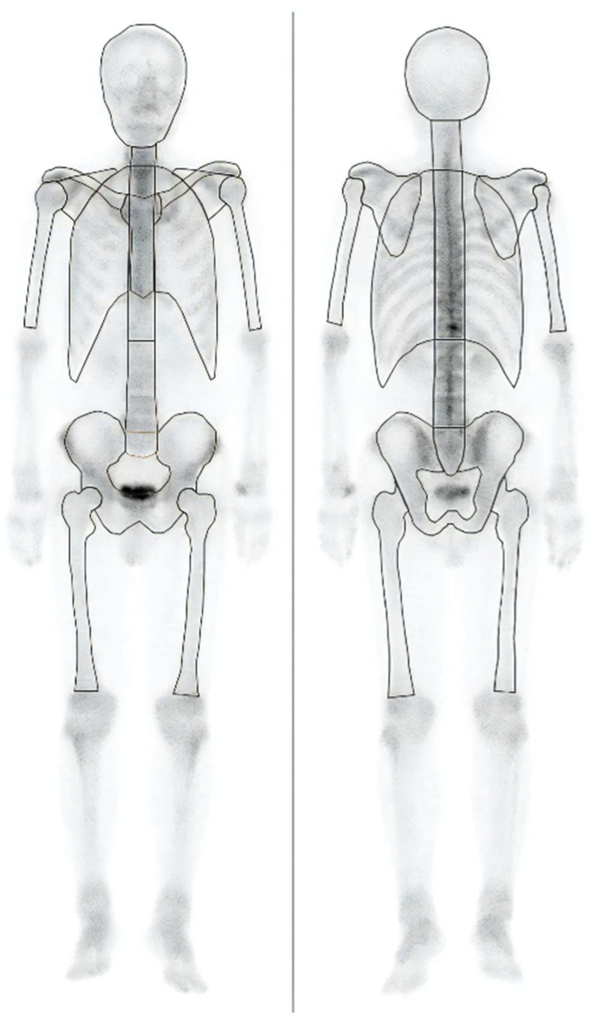
Figure 2.
Distribution of Total-C and Skel-C and the results of significance tests.
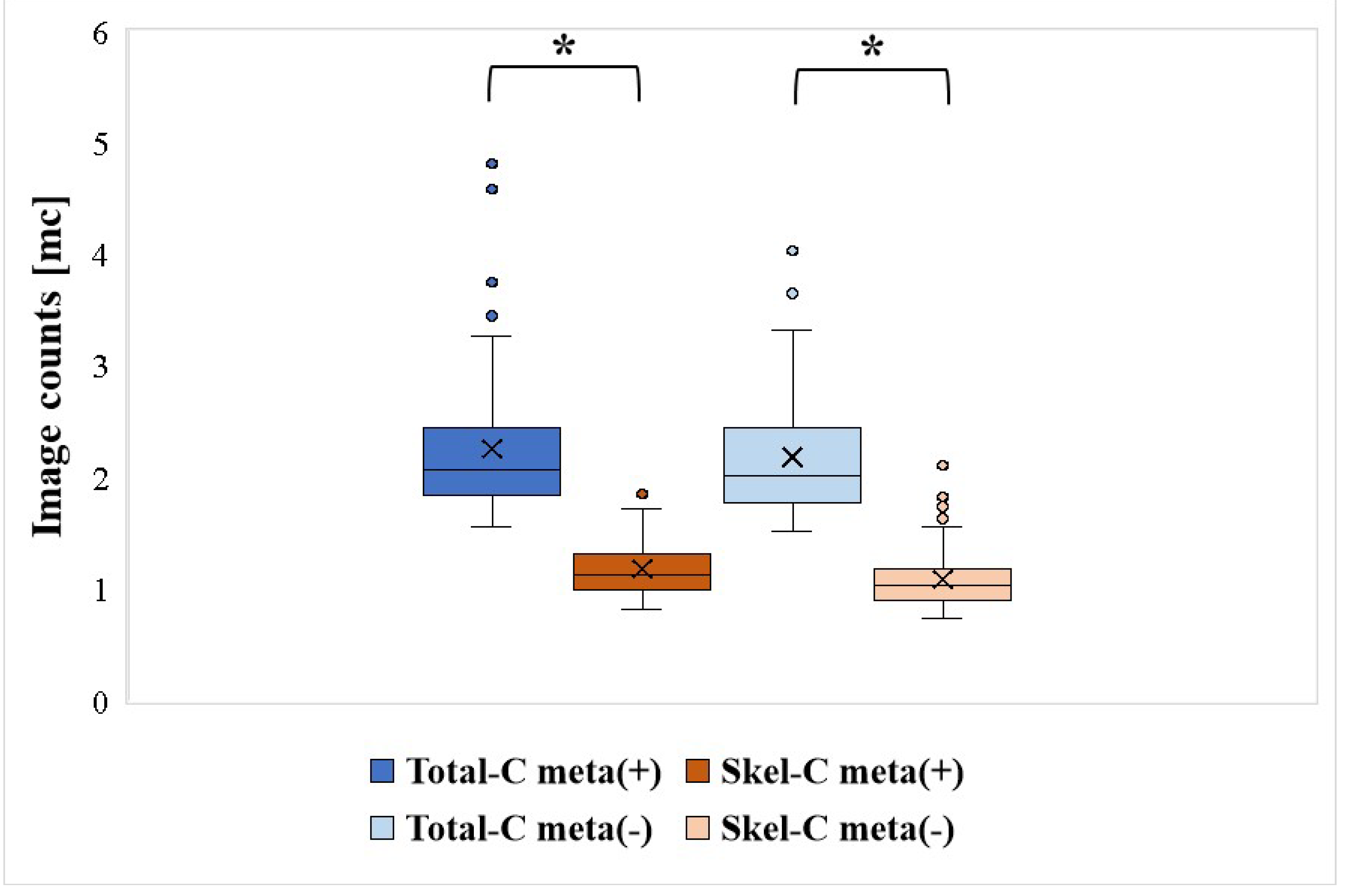
Figure 3.
Sensitivity and significance tests for each group, classified based on the threshold of Skel-C (*: p < 0.05, n.s.: not significant).
Figure 3.
Sensitivity and significance tests for each group, classified based on the threshold of Skel-C (*: p < 0.05, n.s.: not significant).
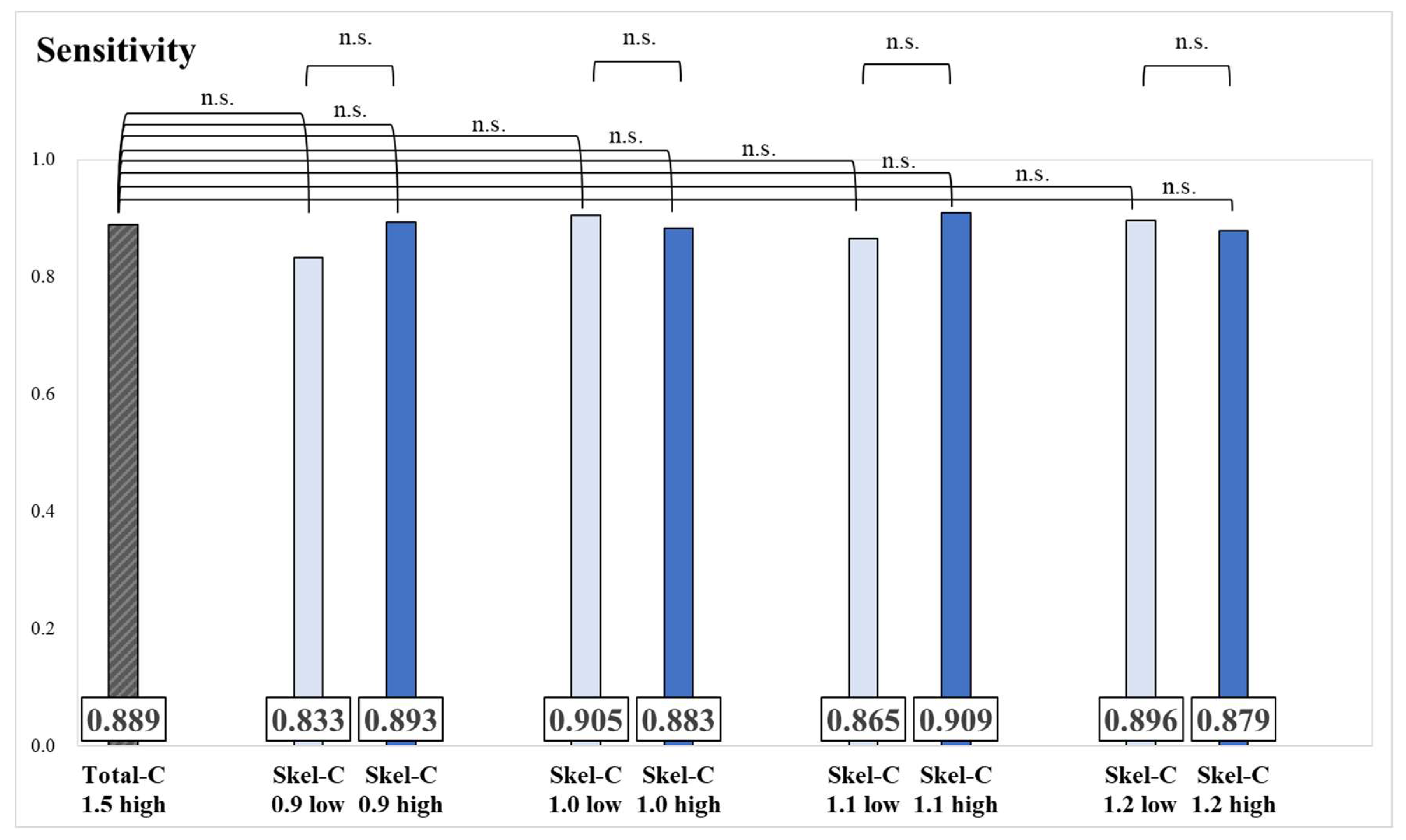
Figure 4.
Sensitivity and significance tests for each group, classified based on the threshold of Total-C (*: p < 0.05, n.s.: not significant).
Figure 4.
Sensitivity and significance tests for each group, classified based on the threshold of Total-C (*: p < 0.05, n.s.: not significant).
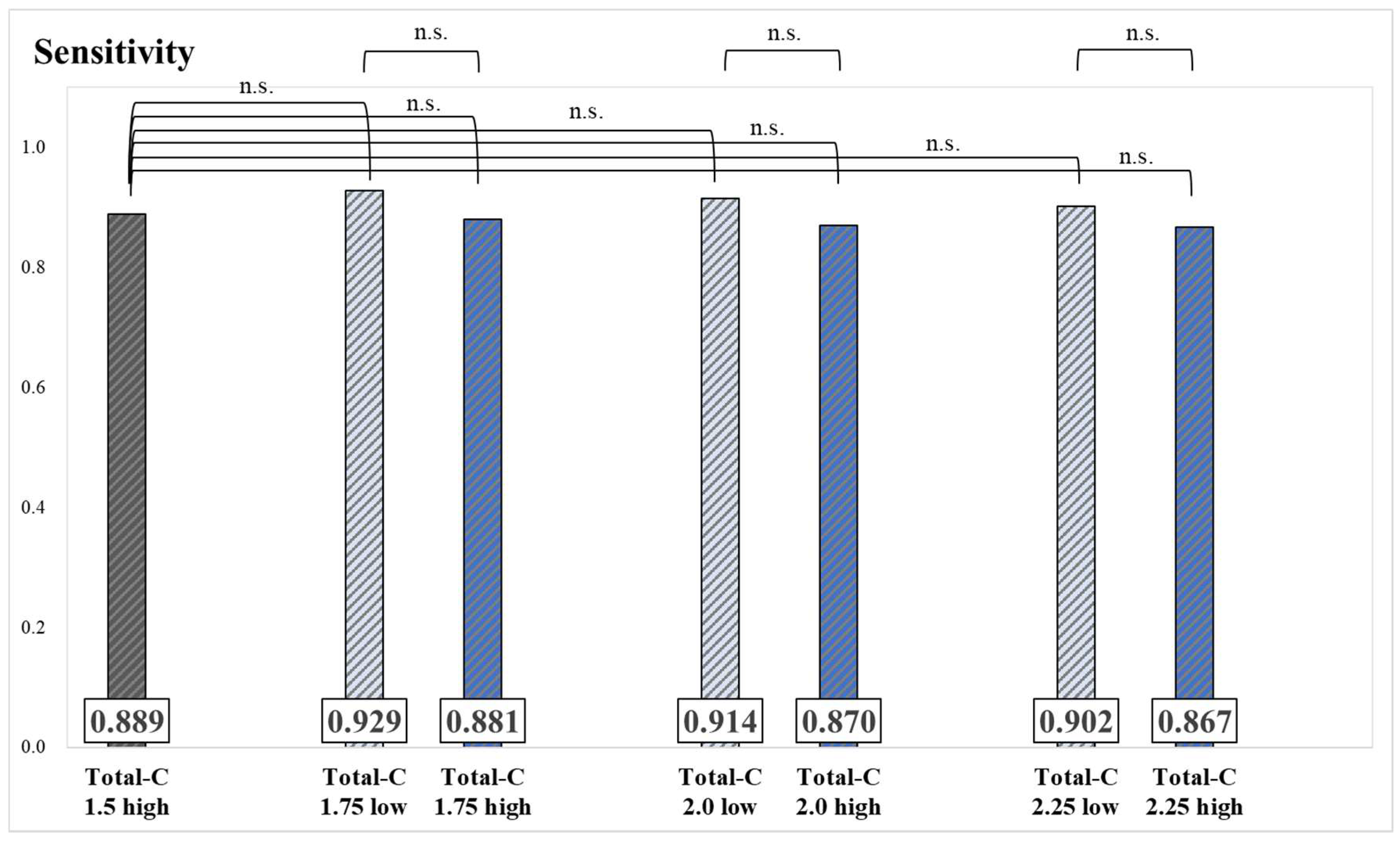
Figure 5.
Specificity and significance tests for each group, classified based on the threshold of Skel-C (*: p < 0.05, n.s.: not significant).
Figure 5.
Specificity and significance tests for each group, classified based on the threshold of Skel-C (*: p < 0.05, n.s.: not significant).
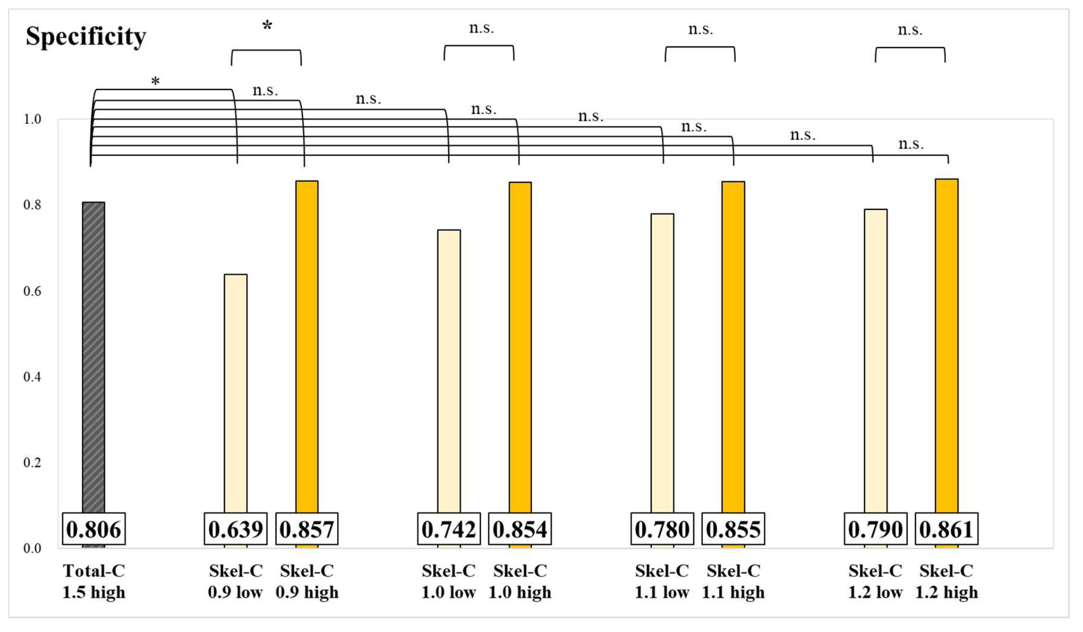
Figure 6.
Specificity and significance tests for each group, classified based on the threshold of Total-C (*: p < 0.05, n.s.: not significant).
Figure 6.
Specificity and significance tests for each group, classified based on the threshold of Total-C (*: p < 0.05, n.s.: not significant).
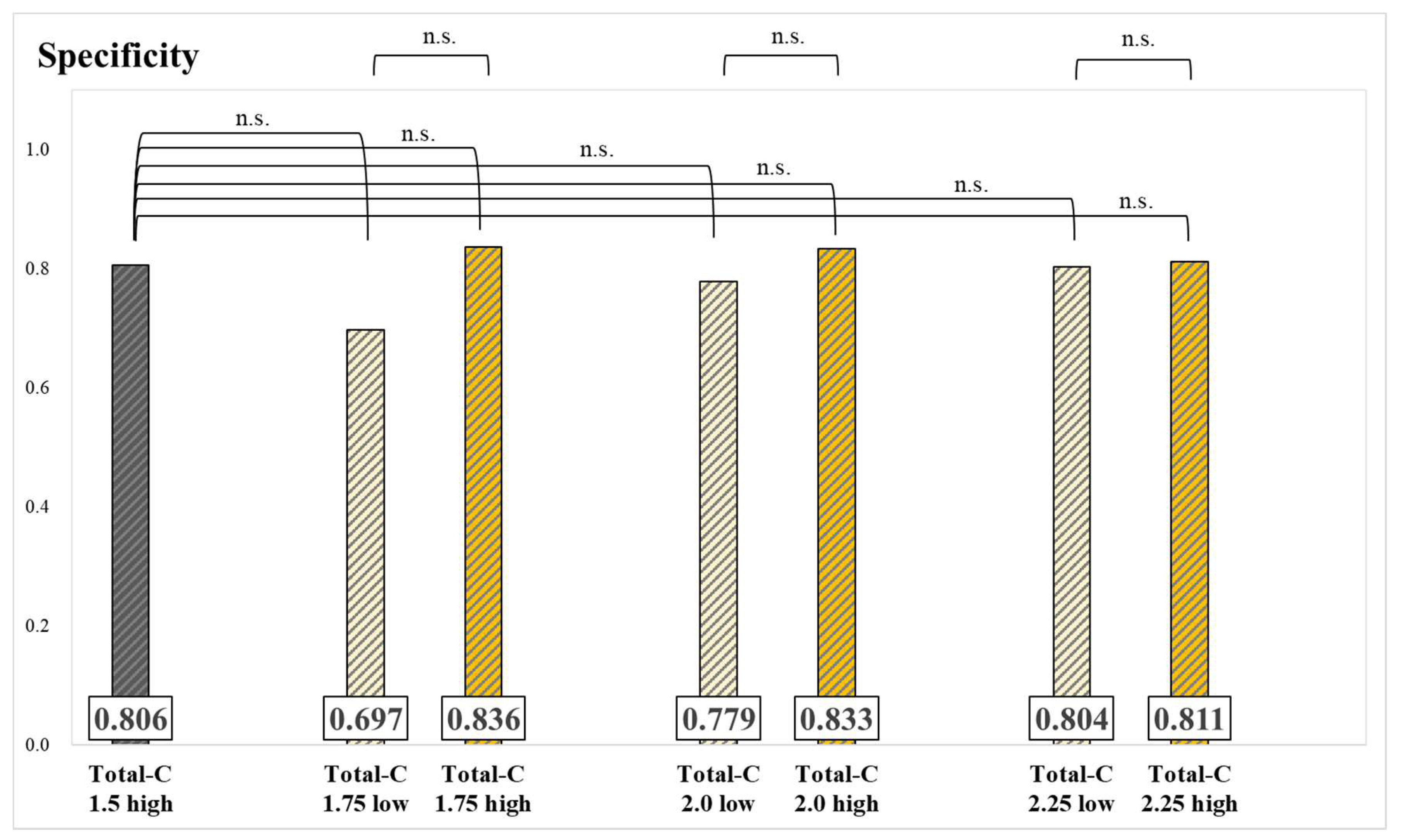
Figure 7.
AUC values and significance tests for each group, classified based on the threshold of Skel-C (*: p < 0.05, n.s.: not significant).
Figure 7.
AUC values and significance tests for each group, classified based on the threshold of Skel-C (*: p < 0.05, n.s.: not significant).
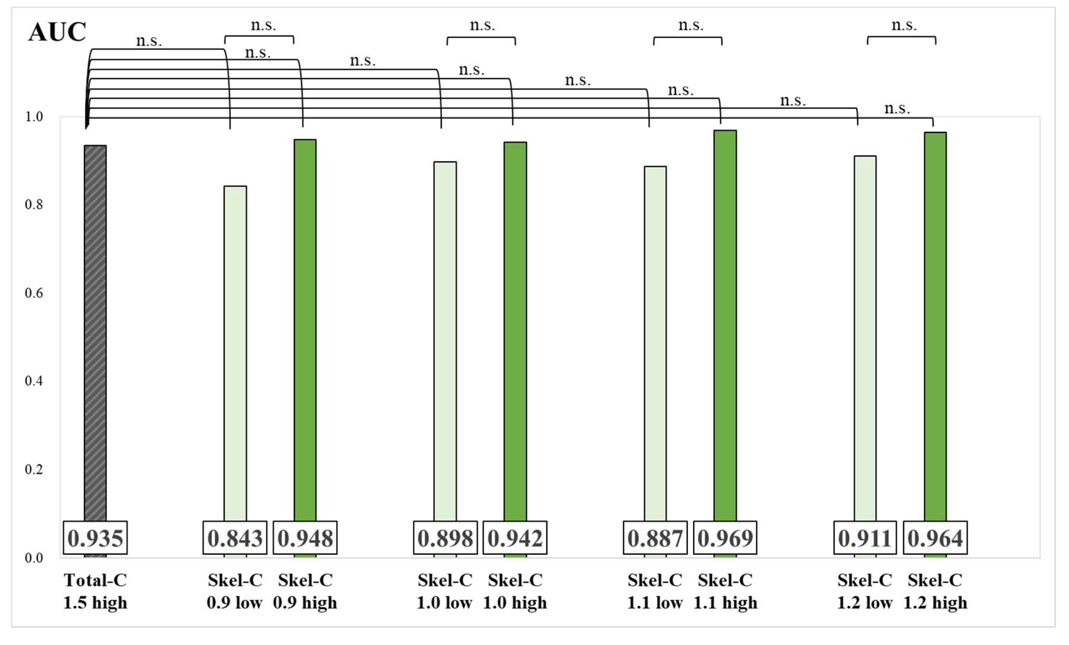
Figure 8.
AUC values and significance tests for each group, classified based on the threshold of Total-C (*: p < 0.05, n.s.: not significant).
Figure 8.
AUC values and significance tests for each group, classified based on the threshold of Total-C (*: p < 0.05, n.s.: not significant).
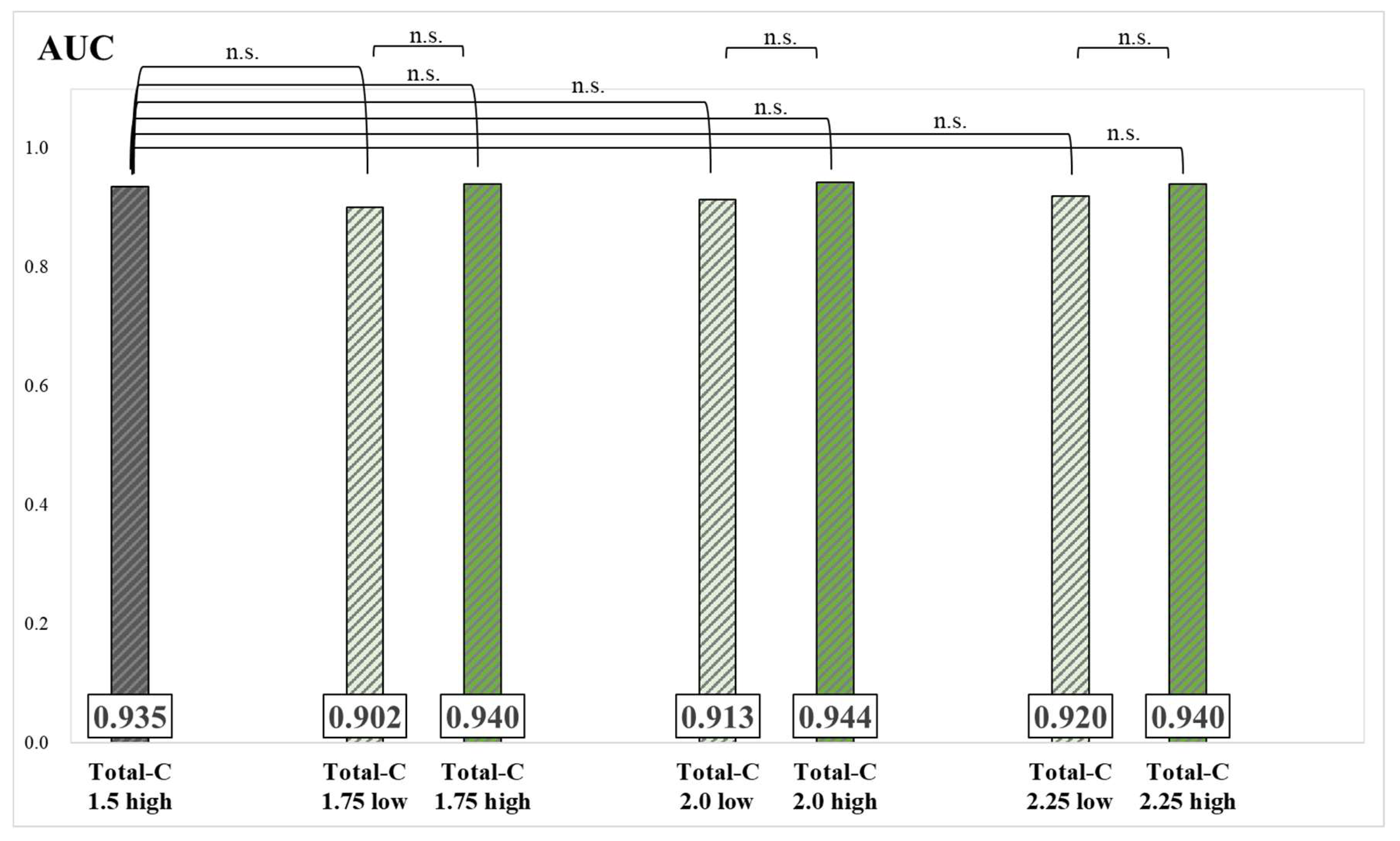
Figure 9.
A case showing a true negative result in BONENAVI. Total-C: 2.37 million count (mc), Skel-C:1.34 mc. (a): results of BONENAVI analysis (b): computed tomography (CT) image (c): single-photon emission computed tomography (SPECT) image.
Figure 9.
A case showing a true negative result in BONENAVI. Total-C: 2.37 million count (mc), Skel-C:1.34 mc. (a): results of BONENAVI analysis (b): computed tomography (CT) image (c): single-photon emission computed tomography (SPECT) image.
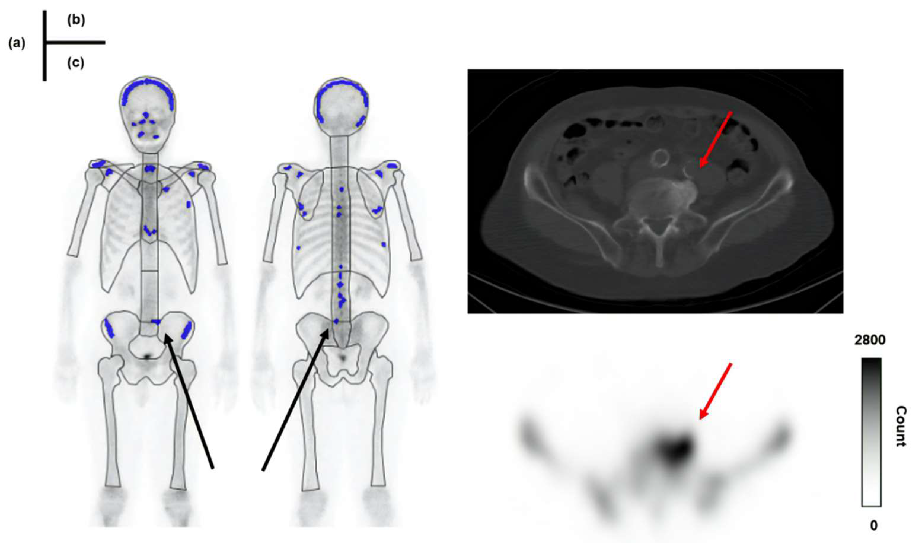
Figure 10.
A patient showing a false-positive result in BONENAVI. Total-C: 3.17 mc, Skel-C:0.89 mc. (a): results of BONENAVI analysis (b): CT image (c): SPECT image.
Figure 10.
A patient showing a false-positive result in BONENAVI. Total-C: 3.17 mc, Skel-C:0.89 mc. (a): results of BONENAVI analysis (b): CT image (c): SPECT image.
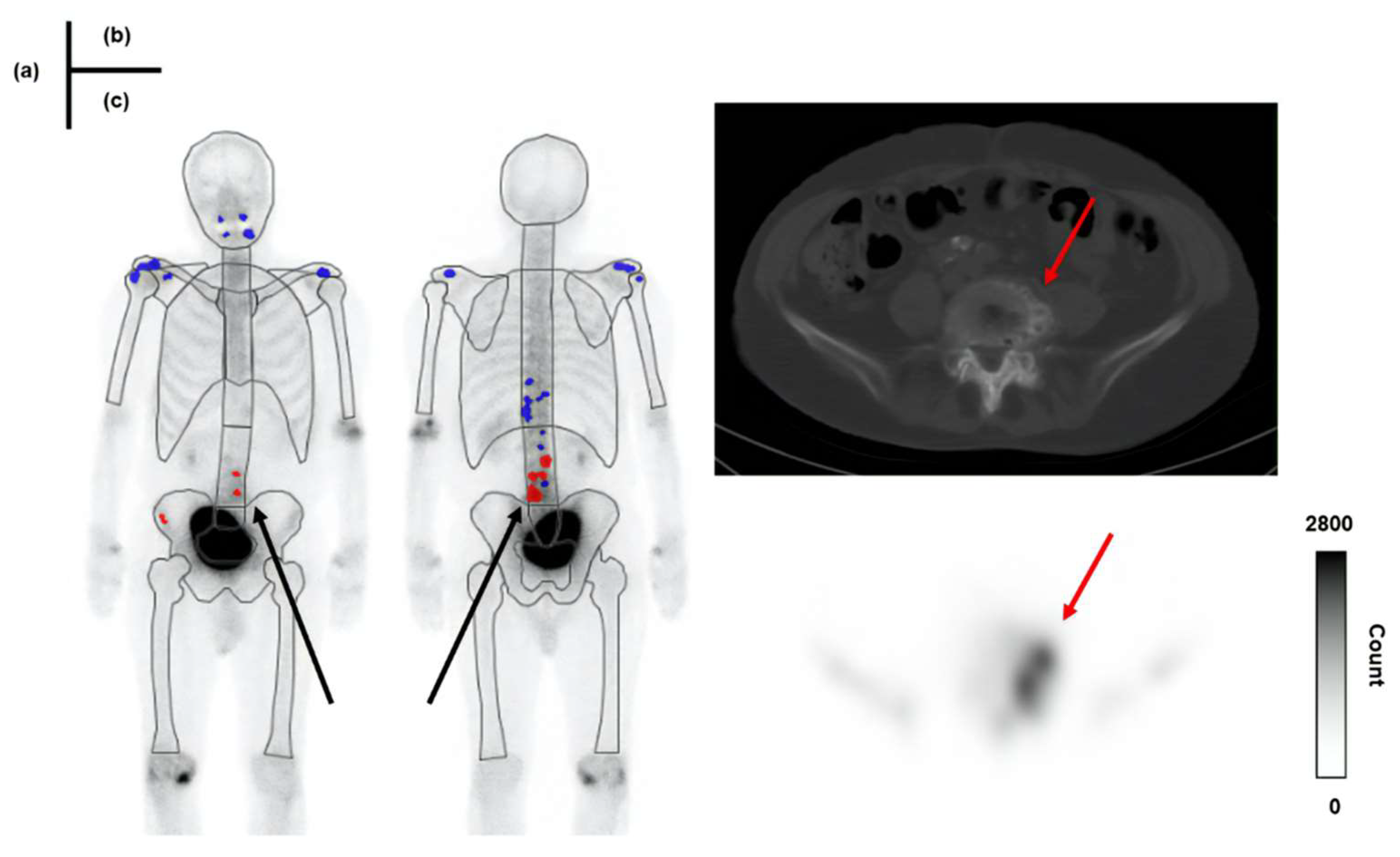
Figure 11.
Distribution of post-injection waiting times and results of significance tests for each group stratified by Skel-C threshold.
Figure 11.
Distribution of post-injection waiting times and results of significance tests for each group stratified by Skel-C threshold.
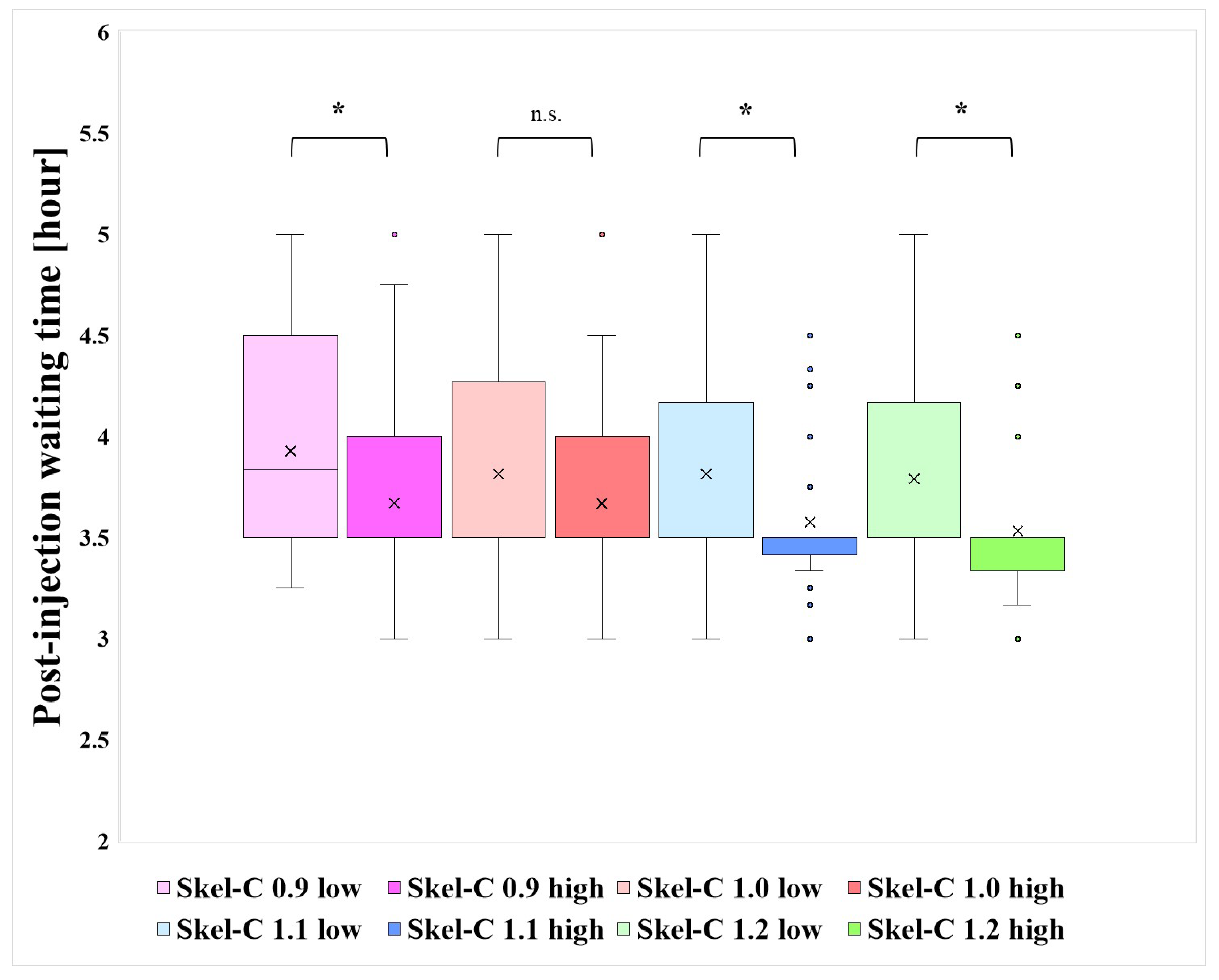

Table 1.
Details of each grouping with the total count (Total-C) and skeletal count (Skel-C) as thresholds.
Table 1.
Details of each grouping with the total count (Total-C) and skeletal count (Skel-C) as thresholds.
| N | Bone meta (+) | Bone meta (-) |
Injected dose [MBq] |
Post-injection waiting time [hour] |
|
|---|---|---|---|---|---|
| Skel-C 0.9 low | 42 | 6 | 36 | 755 | 3.93 |
| Skel-C 1.0 low | 87 | 21 | 66 | 757 | 3.83 |
| Skel-C 1.1 low | 137 | 37 | 100 | 752 | 3.84 |
| Skel-C 1.2 low | 167 | 48 | 119 | 753 | 3.82 |
| Skel-C 0.9 high | 194 | 75 | 119 | 751 | 3.73 |
| Skel-C 1.0 high | 149 | 60 | 89 | 749 | 3.72 |
| Skel-C 1.1 high | 99 | 44 | 55 | 751 | 3.66 |
| Skel-C 1.2 high | 69 | 33 | 36 | 747 | 3.63 |
| Total-C 1.75 low | 47 | 14 | 33 | 757 | 3.88 |
| Total-C 2.0 low | 112 | 35 | 77 | 758 | 3.72 |
| Total-C 2.25 low | 153 | 51 | 102 | 758 | 3.83 |
| Total-C 1.75 high | 189 | 67 | 122 | 758 | 3.68 |
| Total-C 2.0 high | 124 | 46 | 78 | 758 | 3.81 |
| Total-C 2.25 high | 83 | 30 | 53 | 758 | 3.63 |
| Total-C 1.5 high | 236 | 81 | 155 | 752 | 3.76 |
Table 2.
Mean [million count (mc)], median [mc], minimum (Min) [mc], maximum (Max) [mc], and standard deviation (SD) of Total-C and Skel-C grouped by bone metastasis (Bone meta).
Table 2.
Mean [million count (mc)], median [mc], minimum (Min) [mc], maximum (Max) [mc], and standard deviation (SD) of Total-C and Skel-C grouped by bone metastasis (Bone meta).
| Bone meta (+) | Bone meta (-) | |||
| Total-C | Skel-C | Total-C | Skel-C | |
| Mean [mc] | 2.25 | 1.18 | 2.18 | 1.09 |
| Median [mc] | 2.07 | 1.13 | 2.02 | 1.03 |
| Min [mc] | 1.56 | 0.81 | 1.51 | 0.73 |
| Max [mc] | 4.82 | 1.85 | 4.11 | 2.14 |
| SD | 0.63 | 0.23 | 0.54 | 0.26 |
Disclaimer/Publisher’s Note: The statements, opinions and data contained in all publications are solely those of the individual author(s) and contributor(s) and not of MDPI and/or the editor(s). MDPI and/or the editor(s) disclaim responsibility for any injury to people or property resulting from any ideas, methods, instructions or products referred to in the content. |
© 2024 by the authors. Licensee MDPI, Basel, Switzerland. This article is an open access article distributed under the terms and conditions of the Creative Commons Attribution (CC BY) license (http://creativecommons.org/licenses/by/4.0/).
Copyright: This open access article is published under a Creative Commons CC BY 4.0 license, which permit the free download, distribution, and reuse, provided that the author and preprint are cited in any reuse.


