
Submitted:
06 December 2024
Posted:
09 December 2024
You are already at the latest version
Abstract
The combination of BERT and Graph Neural Networks (GNN) has been extensively explored in the text classification literature, usually employing BERT as a feature extractor combined with heterogeneous static graphs. BERT transfers information via token embeddings, which are propagated through GNNs. Text-specific information defines a static heterogeneous graph. Static graphs represent specific relationships and do not have the flexibility to add new knowledge to the graph. To address this issue, we build a tied connection between BERT and GNN exclusively using token embeddings to define the graph and propagate the embeddings, which can force the BERT to redefine the GNN graph topology to improve accuracy. Thus, in this study, we reexamine the design spaces and test the limits of what this pure homogeneous graph using BERT embeddings can achieve. Homogeneous graphs offer structural simplicity and greater generalization capabilities, particularly when integrated with robust representations like those provided by BERT. To improve accuracy, the proposed approach also incorporates text augmentation and label propagation at test time. Experimental results show that the proposed method outperforms state-of-the-art methods across all datasets analyzed, with consistent accuracy improvements as more labeled examples are included.
Keywords:
graph neural networks
; semi-supervised
; text classification
; bert model
; node classification
; graph building
1. Introduction
Text classification is a key task within natural language processing techniques. Many text classification tools rely on a large amount of labeled data to achieve good performance. However, obtaining an acceptable volume of labeled data is expensive. In response, unsupervised and semi-supervised methods have been developed to reduce this dependency, lowering costs while maintaining high accuracy levels.
Combine BERT with Graph Convolutional Networks (GCNs) has been explored in text classification tasks, especially using heterogeneous graphs [1,2,3,4]. These studies adopted heterogeneous graphs because of their rich representation and ability to capture complex data relationships. However, the heterogeneous graphs introduce challenges, such as scalability issues, manual decisions to model relationships between types of nodes, and difficulties in propagating knowledge to the backbone [5].
In this context, homogeneous graphs emerge as a promising alternative, offering structural simplicity and generalization capabilities, particularly when integrated with robust representations like BERT embeddings. However, homogeneous GNN usually has less information, and it naturally has less expressiveness. To alleviate this issue, the proposal introduces a series of text augmentations designed to enhance representational power. Text augmentation has emerged as a relevant strategy to improve semi-supervised learning, which uses unlabeled data to enhance model performance. By generating additional data through transformations of existing samples, data augmentation mitigates overfitting and enhances generalization capabilities [6]. This approach can benefit models based on dynamic graphs, where augmented graphs introduce subtle variations of tokens that enrich the training process, retaining the semantic meaning of the original text.
The semi-supervised learning literature often highlights BERT as a powerful feature extractor, with joint training alongside GNN enhancing capabilities while keeping a static graph topology. This is especially true for TextGCN and BertGCN variants. The proposal better integrates BERT and GNN not only as a feature extractor but also as a guide for dynamic graph construction. This enables the proposal to capture richer semantic information and achieve a more efficient integration between representation learning and graph structure.
Literature reviews on GNNs in texts [7] and semi-supervised setups [8] indicate that many methods still rely on static graphs. Dynamic graph construction is an emerging and important area of interest [9,10,11], especially in computer vision [12,13,14]. In text classification, it is still not extensively explored. Our method introduces the approach to dynamically adapt textual data into graphs using BERT embeddings. Another idea not widely explored in the text domain is label propagation during test time. The unsupervised information of the test batch can be used to improve the graph. The label propagation at test time mechanism can access features test data during the inference, improving accuracy in graph-related tasks [15,16,17,18]. While this characteristic is inherent in some graph scenarios, we have explored a way to integrate these benefits into our proposal.
The main contribution of this study is a semi-supervised technique for text classification named Dynamic Graph with BERT (DynGraph-BERT). The proposal combines text augmentation, dynamic graph construction, and label propagation at test time. This unique combination allows the design of an algorithm to compete with state-of-the-art semi-supervised text classification algorithms based on GNNs.
2. Related Work
Several works seek improvement for text classification on semi-supervised scenario. Recent methods in graph neural networks often use TextGCN [19] as a starting point. TextGCN represents the corpus as a graph, where nodes correspond to words and documents, connected through relationships based on word co-occurrence and word occurrence in document [19]. The model learns text representations by propagating information through graph connections, capturing global semantic relationships [19]. The Heterogeneous Graph Transformer (HGT) [20] was designed to model large-scale graphs, using specific parameters for the node and edge types to perform dedicated attention. It also incorporates relative temporal encoding to capture dynamic dependencies. The HGSampling algorithm, inserted into the method, enables heterogeneous mini-batch sampling, allowing it to efficiently train on large-scale web graphs [20]. Heterogeneous Graph Attention Network (HGAT) introduces a heterogeneous information network (HIN) to model short texts by incorporating additional information and capturing their relationships to mitigate semantic sparsity [21]. Based on the HIN graph, the method applies a two-level Graph Attention Network (GAT) — node-level and type-level — to learn the relationships between neighboring nodes, optimizing short text classification in a semi-supervised scenario [21].
The Short Text Heterogeneous Graph Network (STHGN) is a self-supervised method for short text classification that addresses the lack of information in the corpus by modeling it as a heterogeneous graph [22]. It employs a self-attention-based heterogeneous graph neural network (SAHGNN) to learn embeddings for short texts. Additionally, it implements a self-supervised learning framework to explore both internal and external similarities among texts [22]. Heterogeneous Graph-Convolution-Network-Based Short-Text Classification (SHGCN) constructs a heterogeneous graph using nodes representing entities and words, connected through mutual information and confidence between documents, words, and entities. The features are represented within a word graph, combined with BERT embeddings, and further enhanced using a BiLSTM [23].
TextGCN, HGAT, STHGN, SHGCN, and VGCN process data using a static graph, limiting their ability to discover additional node patterns during training by enhancing knowledge between epochs. HGT operates with dynamic graphs but ignores the embedding information of pre-trained models.
Another interesting algorithm is InducT-GCN [24]. As an inductive approach, this study constructs the graph exclusively using training data, enabling the model to train without relying on any information from the test set. The graph nodes are divided into two types – nodes representing documents and those representing unique words in the training documents. The features are one-hot vectors for words and Term Frequency-Inverse Document Frequency (TF-IDF) for documents, enabling alignment between the two. The two types of edges: words with words, based on Point-Wise Mutual Information (PMI) considering the co-occurrence of connected words; and documents with words, if the word is in the text, then connect them, determined by TF-IDF values. Induct-GCN relies solely on internal information and does not employ transfer learning to achieve higher accuracies. When unknown words are encountered, this information is excluded from the graph and the model, making it heavily dependent on the training data.
As already mentioned, most of the methods use static graphs, and the term frequency text representation is still the preferred strategy in the literature found to build the graphs. In this work, we seek to follow a different avenue. We re-examine the design spaces and test the limits of what a pure homogeneous graph can achieve. The proposal focused on the expressiveness of BERT enhanced by data augmentation and transductive at test time approach. We also observe that the relationship of the documents at batch has not been explored in the form of label propagation at test time in these methods. Considering these research gaps, we propose DynGraph-BERT.
3. Preliminaries
3.1. Graph Neural Network
Graph Neural Networks (GNN) have gained popularity largely through the works of [25] with convolutional in graph neural networks. This technique represents a combination of artificial neural networks tailored to handle structured data in graphs. The benefits of using graphs to structure data lie in the increased information gain compared to tabular data, as graphs are not confined to themselves; they enable the relationship between one data point and others, unveiling new associated or underlying patterns among them [26]. However, they introduce other challenges such as data heterogeneity within the graph [27,28], generalization of learned knowledge to new graphs, efficient data propagation, and the trade-off between model accuracy and computational efficiency [24,28,29,30,31], over-smoothing, under-reaching and over-squashing [31].
A Graph Neural Network is a machine learning framework that models and analyzes structured data through graphs. A graph G is an ordered pair , where V represents a set of nodes, and E represents a set of edges that link the nodes. A GNN is a parametric model consisting of multiple layers, where each layer deals with the aggregation of information from neighboring nodes and edges.
The fundamental operation of GNN involves aggregating information from the neighbors of a node and subsequently updating the representation of that node. This process is performed iteratively across l layers. At each layer, the representation of a node , denoted as , is updated based on the aggregation of information from its neighbors, , as defined in Equation (1).
The Equation (2) represents the node updated using the aggregated information from its neighbors [32].
The aggregate function can be a mean, sum, min, or max from its neighbor features’ values [33]. The update function is generally a feedforward neural network. In the case of GCN, the update function takes the following Equation (3) to update the layers [34]:
is the weight matrix of layer l, which will be learned during training, f is a non-linear activation function, is the normalized adjacency matrix of the graph as shown in the Equation (4). D is the diagonal degree matrix of the layer l, where . The normalization by avoids scaling issues of values during propagation. The identity matrix includes self-loop connections. The first layer is the features of data.
Through multiple layers, a GCN can effectively learn to incorporate information from the neighborhoods of nodes, allowing the capture of complex features of data structured in a graph.
The loss function is defined as the cross-entropy error over all labeled documents [34]:
where is the set of text indices that have labels and C is the dimension of the output features, which is equal to the number of classes. Y is the label indicator matrix.
3.2. Transductive Versus Inductive
In a node classification problem of a graph, let V be the set of nodes and E the set of edges of a graph . In inductive learning, we are interested in learning a function such that , where Y is the set of labels for each node.
The training space of an inductive model is defined by a graph such that and where and are, respectively, the sets of training nodes and the set of edges that connect nodes in . The set of edges can be defined as . In the transductive setting, the model has access to all the data (train, test) features, except the class values for testing.
Thus, the training input for the GNN network in an inductive approach is only the graph and . Compared to the transductive approach, the training input graph for the GNN network is formed by and . The advantage space is created by having full access to V and E during training. The adjacency matrix during training in inductive mode is sized , while in transductive mode, it is .
At the end of training in an inductive model allows the creation of edges where and , or the addition of new nodes (representing new samples from the real world). In contrast, the transductive model already determined the classes for all nodes. If new data is introduced to a transductive model, the model must be retrained with this data.
The transductive scenario occurs when the unlabeled test data is at our disposal during the training stage. The access to unlabeled test data usually gives some advantage to transductive in terms of accuracy when compared with inductive. This handy improvement comes with the price. Transductive the model cannot predict future data, only present and past data. Therefore, transductive setup is less common in real-world scenarios. Inductive can be applied in more general setups and applications.
Much related work is on transductive setup, not on inductive setup. It is not always trivial to convert a transductive graph method to an inductive graph method. In most cases, transductive methods incorporate graph-building mechanisms within their training procedures, making the direct conversion to inductive methods difficult. For this reason, we design the proposal in an inductive setup. However, we took advantage of some ideas for the transductive setup using label propagation at test time.
4. DynGraph-BERT
The DynGraph-BERT is a welcome combination of three ideas: data augmentation, dynamic graph construction, and label propagation at test time. In the following sections, we will dive into these topics, followed by the proposal algorithm.
4.1. Data Augmentation
To address the lack of labeled data, we employed two data augmentation techniques. The first involves augmenting data at the text level by modifying words and their structure, using the library nlpaug1 [35]. The second technique is applied to the model-trained embeddings by adding noise to the embedding vectors. Further details about the first technique are provided in the following paragraphs, while the second is discussed at the end of this section.
The nlpaug library provides various strategies for text modification. These techniques increase the variability of the dataset without introducing significant semantic bias, enhancing the robustness of the model when handling noise and variations in text. Specifically, we applied four main approaches:
- Swap: replacing words with synonyms
- Omitting: omitting arbitrary words
- Typos: introducing typos
- Change order: altering the order of words in a sentence
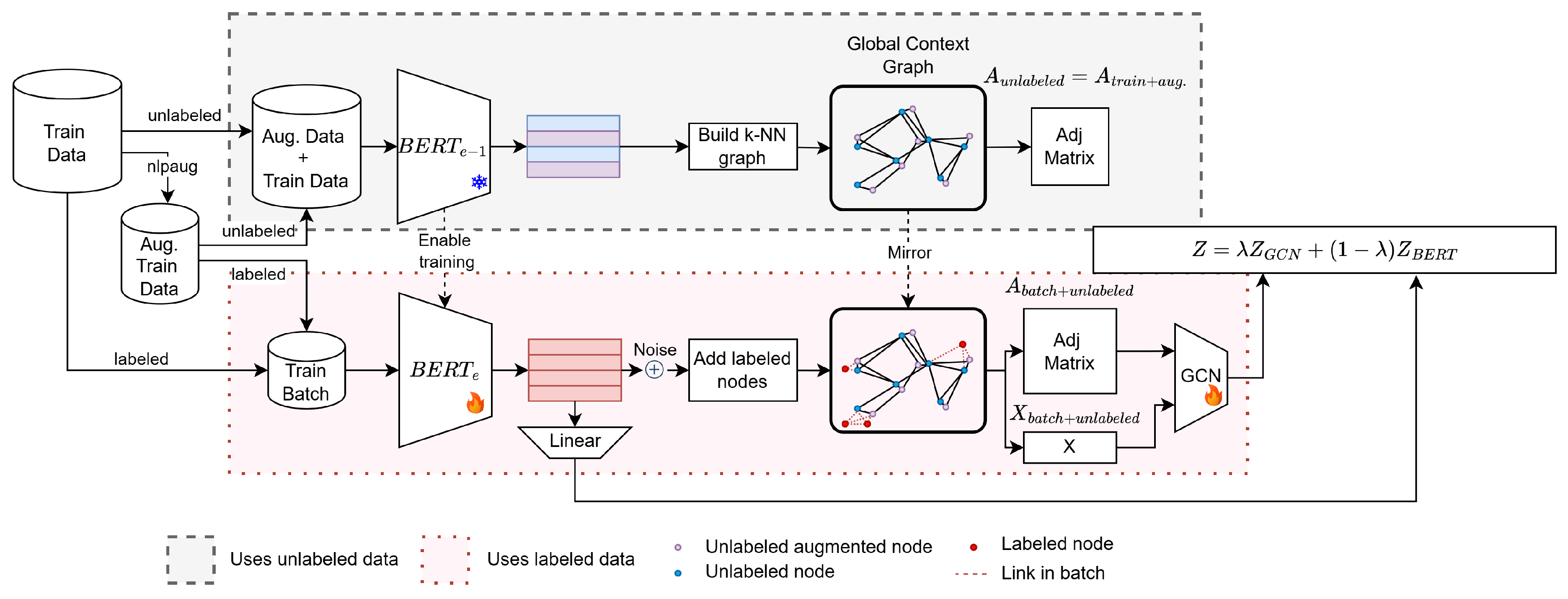
Table 1 presents examples of these transformations, demonstrating how these techniques preserve the overall meaning while enhancing dataset diversity. The selection of these techniques balances computational costs and performance improvement [36,37]. Data augmentation with nlpaug has two application points, as illustrated in Figure 1 within the cylinder labeled Aug. Train Data. The first application contributes to creating the Global Context Graph, represented in the gray space in Figure 1. The second is actively integrated into the training process through batches, represented in the red space in Figure 1.
The data augmentation process yields two outcomes: the augmented data, which is incorporated into the batch training process, and the augmented graph, comprising unlabeled training data alongside augmented unlabeled data. An evaluation of both outcomes will be conducted in the ablation study section.
Noise augmentation data are introduced to produce augmented embeddings, improving the robustness of embeddings, as denoted by [38,39]. This noise is a small variation applied to each dimension of the embeddings, represented by a vector of the same size as the embeddings. The adjustments in each dimension are minor and follow a normal distribution, as described in Equation 7.
represents the i-th original embedding, is the normal distribution with mean and variance . The noise is applied to both CLS and AVG embeddings during train steps and will be explained in detail later.
Figure 1.
Overview of the DynGraph-BERT training process for a single epoch.
4.2. Dynamic Graph
The dynamic graph plays a critical role in both the training process and the prediction of nodes within the graph. Its construction begins with what we call the Global Context Graph. In this graph, nodes represent texts, and their features are embeddings generated by a frozen BERT model, denoted . This ensures that the initial feature representations remain consistent throughout the construction phase.
Textual data represented as , where i is the index of the text in the training dataset, is processed by with all layers frozen, that is, its parameters are locked. The encoder output produces the feature representation , as described in Equation (8). Each resulting embedding vector is associated with a node , . The embeddings used in the graph construction are average embeddings (AVG embeddings) derived from the output of the last BERT layer, including the CLS token. Including the CLS token is justified as BERT encodes class information within this embedding, making it a valuable feature for downstream tasks [40].
The connections are based on their embeddings and nearest neighbors. Edges are added under two conditions: a specified number of nearest neighbors k and a minimum similarity threshold m, both configurable hyperparameters. The similarity is quantified as the inverse of the cosine distance between the text embeddings, as defined in Equation (9). The resulting graph is weighted, with each edge’s weight corresponding to the calculated similarity.
In the training process, the dynamic nature of the graph is introduced. During each epoch, the model processes data in batches. For each batch, new embeddings are computed by a trainable BERT model, which is fine-tuned for the classification task. These embeddings are perturbed with augmented noise and added to the Global Context Graph following the same edge rules. As a result, a unique batch-specific graph is generated for training, as illustrated in Figure 2a. This batch graph is processed by a GCN, which refines its weights based on the classification task.
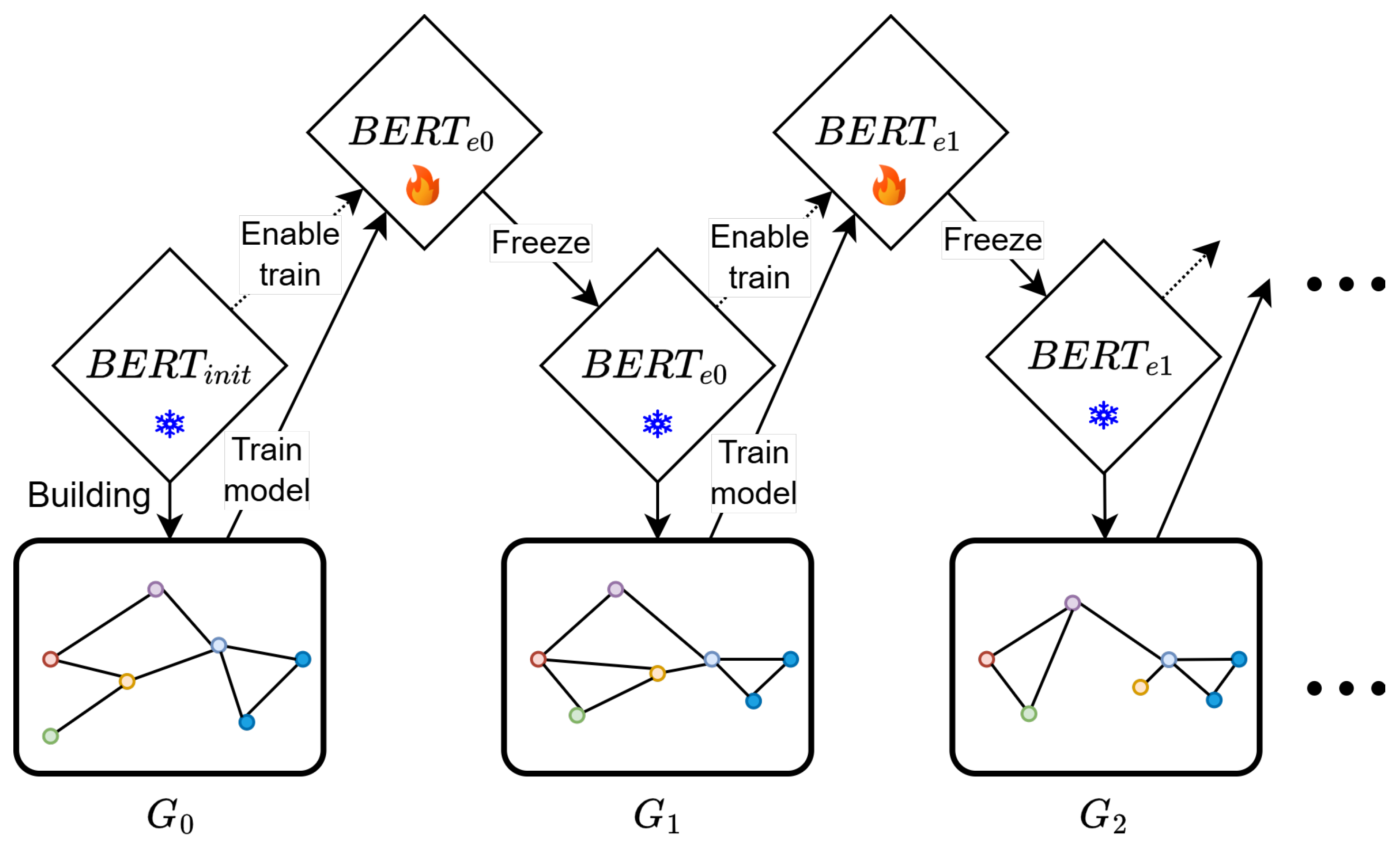
At the end of each epoch, the embeddings in the Global Context Graph are recalculated using the updated BERT model. This process creates a new Global Context Graph () at the beginning of each subsequent epoch. Each graph incorporates the knowledge gained during the previous epoch, allowing the model to adapt dynamically and integrate new insights. Figure 3 depicts the evolution of the Global Context Graph across epochs.
This iterative approach offers several advantages. First, it enables the model to incorporate dynamic changes in the representation of textual data, improving its ability to generalize. Second, it facilitates the creation of transductive graphs during the test time, leveraging information from the training process.
Figure 3.
Overview of the DynGraph-BERT training process across epochs. Colors in the graph represent node identification.
Figure 3.
Overview of the DynGraph-BERT training process across epochs. Colors in the graph represent node identification.
4.3. Label Propagation at Test Time
The graph is built following the same creation rules mentioned earlier, adhering to the specified number of k neighbors and a minimum similarity threshold. Label propagation occurs when the unlabeled test data are included in the graph. This allows any test example to contribute to the batch being predicted. In Figure 2b, this is illustrated with the graph of , which includes unlabeled test data in yellow, unlabeled training data in blue, and the batch examples to be predicted in green.
The information propagation now also flows using unlabeled test data (yellow dots). In this way, the unlabeled test data can propagate the information through the graph, helping the GCN to improve the classification task (see the Ablation section).
4.4. DynGraph-BERT Algorithm
DynGraph-BERT is a graph-based model integrating GCN and BERT in an inductive setup with a homogeneous graph and semi-supervised learning. Its semi-supervised nature emerges from graph construction without labels or external data during both the training and testing phases. Algorithm 1 outlines the procedural steps involved in the training process, whereas Algorithm 2 delineates the methodology for evaluating the model.
Recap the steps with data augmentation, at lines 1 and 2, the graph augmentation is built with the rules of k and m at line 4 in Algorithm 1. The encoder , at line 5, is activated for training, indicated by a flame icon in Figure 1. Each text segment is encoded, generating CLS-position embeddings for classification, as in a traditional BERT model. Additionally, AVG embeddings are incorporated into the training graph, following the k-neighbor constraint and a minimum similarity threshold m. This process is depicted as build k-NN graph in Figure 1.
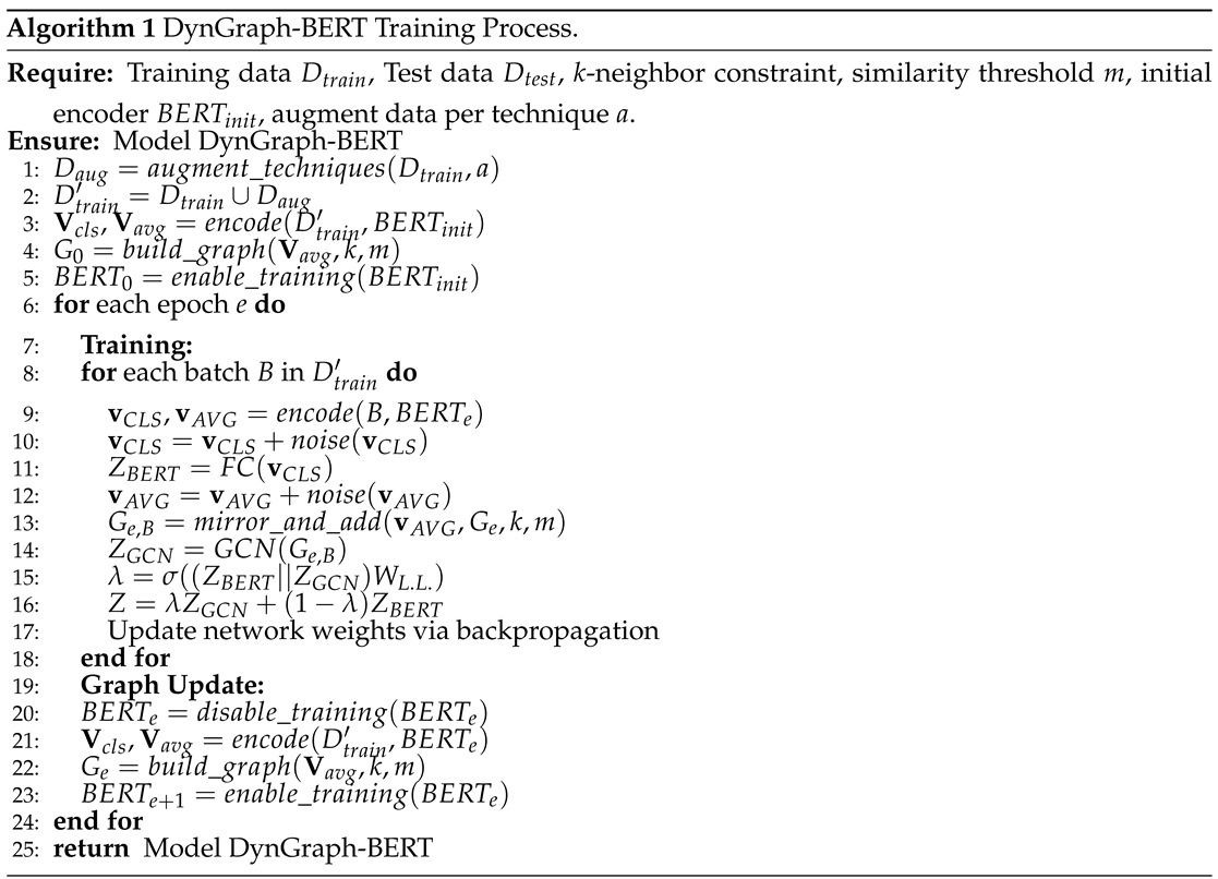 |
After graph construction, the learning flow resumes, updating network weights through batches. In the standard BERT flow, the CLS embedding passes through a fully connected (FC) layer, resulting in BERT logits. In the graph-based flow, AVG embeddings serve as graph features processed by two GNN layers, producing GNN logits. The final logits are computed as a weighted combination of the two. To regulate model learning, a Lambda Learner (L.L.) mechanism is integrated. This mechanism determines using a linear layer that learns the optimal value for each text segment. The input to this mechanism comprises embeddings from both flows concatenated as described in Equation (12):
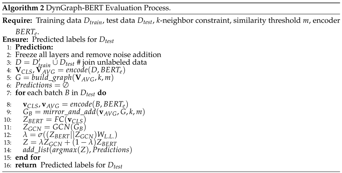 |
For evaluation, the examples to be predicted are processed in batches, all layers are frozen, and noise addition is omitted. The model generates AVG embeddings for graph construction, which are used to create new AVG and CLS embeddings for each test batch. The graph construction for prediction includes both training data and evaluation data, maintaining the same k and m values. For each batch in the evaluation set, CLS embeddings are classified through an FC layer, while AVG embeddings are processed by a GNN. The logits from both flows are combined using the value for each batch, as shown in Figure 4. The final prediction is obtained by an ArgMax function on the weighting of the logits.
The model selected for the prediction of the test set corresponds to the best epoch during training, based on the highest accuracy achieved on the validation set. This model is indicated as in Figure 4 and replaces the encoder in the Algorithm 2.
5. Results
Experiments were conducted on five well-known text classification datasets, following the experimental setup of [22]. Ohsumed [41] contains titles and abstracts of medical articles, R8 [19] is a subset of the Reuters news dataset, Snippets [42] comprises search keywords, AGNews [43] is another news dataset, and DBLP [44] consists of text about scientific articles. The dataset size, number of classes, and distributions of examples across training, validation, and test sets are detailed in Table 2.
We processed the text with a BERT tokenizer, using all available words and characters, because BERT was trained with raw text, also [45]. For each dataset, we set the maximum number of tokens, based on a percentile 90% of the length of texts. To build the graph, we used and for the threshold, after a Bayesian hyperparameters search based on the best validation accuracy. The Table 3 shows the other hyperparameters. The learning rate for BERT and GNN was established with the best values of [2]. We used AdamW as an optimizer and applied the warm-up following [2].
To evaluate the performance of DynGraph-BERT, we selected several baseline methods that use graphs in a semi-supervised setting for text classification, including TextGCN [19], HGT [20], HGAT [21], and STHGN [22]. Additionally, we included classical CNNs [46] for comparison purposes.
All benchmark results were sourced from [22]. Ten rounds of experiments were conducted as in [22], and the average accuracy is reported in Table 4. [22] did not provide the code or random seeds used to generate the training and test subsets. It only stated that the subsets were selected randomly from the respective sets was stated. To ensure reproducibility, we attempted to replicate this process in a similar way and recorded the seeds used in the experiments.
Evaluating the methods, DynGraph-BERT surpasses the second-best competitor by more than 3% on the Ohsumed and DBLP datasets and by more than 20% on the Snippets dataset. Even in larger datasets such as Snippets and DBLP, DynGraph-BERT consistently achieves superior performance, with an advantage of over 10% compared to the other methods.

Table 4.
Classification accuracy on the test set based on the training percentages indicated in the parenthesis at the table heading. The best results and second best are in bold and underlined, respectively. The asterisk (*) indicates a significant difference (p < 0.05) with STHGN using a t-test.
Table 4.
Classification accuracy on the test set based on the training percentages indicated in the parenthesis at the table heading. The best results and second best are in bold and underlined, respectively. The asterisk (*) indicates a significant difference (p < 0.05) with STHGN using a t-test.
| Method | Graph type | Ohsumed (2.8%) | R8 (1.04%) | AGNews (0.5%) | Snippets (0.52%) | DBLP (0.5%) |
|---|---|---|---|---|---|---|
| CNN-rand | No graph | 34.07±0.57 | 79.52±1.07 | 39.04±3.74 | 42.41±2.47 | 36.94±1.40 |
| CNN-pretrain | No graph | 22.77±0.56 | 72.41±1.33 | 33.00±1.61 | 52.56±0.95 | 28.64±0.67 |
| TextGCN | Heterogeneous | 28.77±0.39 | 76.15±0.45 | 56.81±1.48 | 35.80±0.59 | 40.01±0.58 |
| HGT | Heterogeneous | 42.44±0.38 | 80.88±1.10 | 31.52±2.66 | 45.42±0.94 | 43.07±0.45 |
| HGAT | Heterogeneous | 39.42±1.26 | 86.45±1.33 | 63.40±4.97 | OOM | OOM |
| STHGN | Heterogeneous | 44.64±0.56 | 90.20±0.73 | 73.41±2.29 | 55.81±1.49 | 46.39±0.81 |
| DynGraph-BERT | Homogeneous | 48.34 *±1.54 | 90.93±1.71 | 83.56 *±1.97 | 77.87 *±3.90 | 58.96 *±2.01 |
OOM is out of memory.
Numerically, DynGraph-BERT shows a higher classification accuracy in all datasets tested. We perform a significance test using a t-test with a p-value < 0.05 to compare our proposal with the state-of-the-art STHGN. The results indicate that we can reject the null hypothesis that DynGraph-BERT and STHGN have similar results with p < 0.05 in four out of five datasets. Statistical analysis was conducted for 6 methods with 50 paired experiments, 10 for each dataset. We remove HGAT because we are unable to run it due to lack of memory.
Therefore, these results indicate that the proposal has higher accuracy in all datasets tested. When comparing DynGraph-BERT and STHGN using the T-Test, we can reject the null hypothesis in four out of five datasets, showing superior results of the proposal.
6. Ablation
This section explores approaches to assess stability and identify key components contributing to model performance. We conducted three experiments: analyzing performance with varying numbers of training examples, evaluating performance by method components, and examining hyperparameter variations.
6.1. Training Sample Size Variation
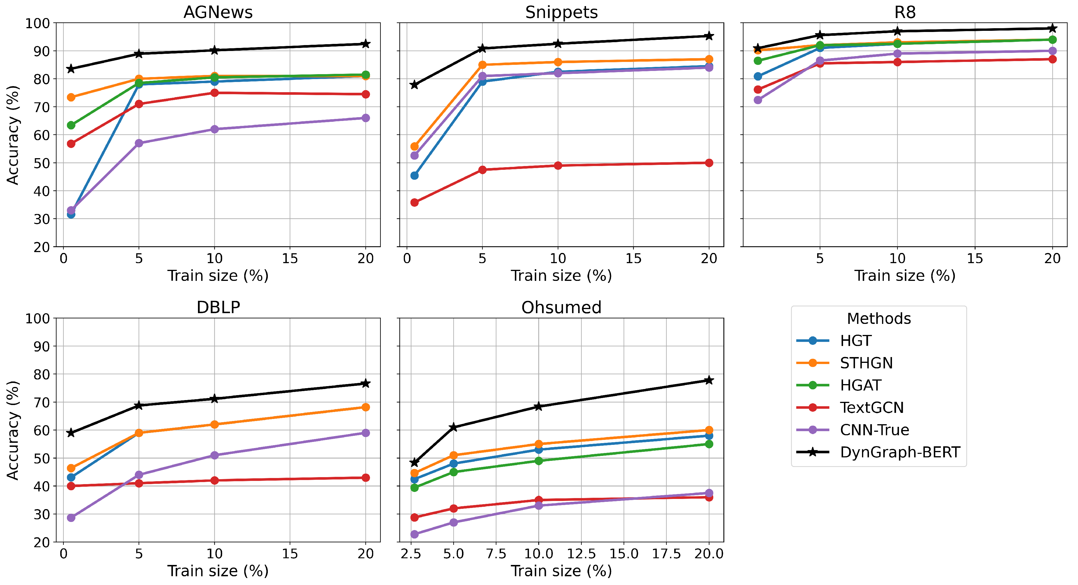
We first evaluated the model’s performance on five datasets with different training sample sizes. Following the experimental setup from [22], we varied the number of examples to 5%, 10%, and 20%, in addition to those already reported in Table 4 and plot the respective accuracies in Figure 5. The results for the other methods were also extracted from [22]. This study examines the impact of data quantity on the generalization capability of the model.
In Figure 5 the proposal (black lines with stars) showed higher accuracy in all tested datasets in all training size percentages. A notable result is observed on the Ohsumed dataset, where increasing the training examples from 2.5% to 20% leads to a 22-point accuracy improvement. Meanwhile, other methods fail to surpass the model’s performance achieved with only 5% of the training data.
Figure 5.
Accuracy results for training data increments.
6.2. DynGraph-BERT Components
To evaluate the impact of different components in our model, we conducted experiments with specific variations, removing or adjusting each component separately, using the same train size reported in Table 2. The average results from 10 runs are reported in Table 5. The variations and components are as follows:
- BERT: The accuracy of the BERT model significantly decreases when dealing with a small number of samples per class.
- model v1: This experiment examines the BERT model enhanced with augmented data. Although this data augmentation contributes to model improvement, the interrelationship between datasets yields superior results compared to subsequent versions of the models.
- model v2: The model was evaluated without data augmentation, using only the original data. It was observed that the DynGraph-BERT model experiences a performance drop, suggesting that augmented data helps with the model’s regularization and robustness.
- model v3: Noisy data was removed during training. The results were quite similar to those of the full method, suggesting that the Aug. Noise is the element with a less contribution to the model’s accuracy.
- model v4: The transductive at test time was excluded. The results show a slight loss in accuracy. This indicates that label propagation in testing remains an advantageous factor in capturing relationships between data, including test data.
- model v5: Data augmentation was performed without additional labeling of the augmented data. Here, the performance was close to that of the full method, showing that this component can be omitted, allowing more unlabeled data to be included while maintaining accuracy.
- model v6: In this case, we evaluated the impact of the dynamic graph. We freeze the BERT model, resulting in the same graph across all training epochs.
The most effective and contributing component is the graph construction and GNN processing, followed by augmented data. The label propagation at test time yields a modest improvement in overall average performance. Labeling the augmented data or adding noise provides minimal improvement. Together, these components make the model more robust than BERT, even when using labeled augmented data.
Table 5.
Table with ablation study.
| Aug. Graph | Dynamic Graph | Aug. Train | L.P.T.T. | Aug. Noise | Ohsumed | AGNews | |
|---|---|---|---|---|---|---|---|
| BERT | - | - | - | 9.53 | 52.12 | ||
| model v1 | - | - | ✔ | - | 37.30 | 81.79 | |
| model v2 | ✔ | ✔ | ✔ | 43.12 | 81.98 | ||
| model v3 | ✔ | ✔ | ✔ | ✔ | 47.31 | 83.46 | |
| model v4 | ✔ | ✔ | ✔ | ✔ | 44.06 | 80.37 | |
| model v5 | ✔ | ✔ | ✔ | ✔ | 45.69 | 81.97 | |
| model v6 | ✔ | ✔ | ✔ | ✔ | 29.20 | 82.45 | |
| proposal | ✔ | ✔ | ✔ | ✔ | ✔ | 48.34 | 83.56 |
Notes: Aug. Graph means Augmented Graph. Aug. Train means training data was augmented. L.P.T.T. means label propagation at Test Time. The bold values represent the best results for the dataset, while the second-best results are underlined.
6.3. Hyperparameter Evaluation
To understand the influence of hyperparameters on the method, we evaluated the minimum similarity level and the maximum number of k neighbors in experiments with the Snippets dataset. The results, averaged over 10 runs of the DynGRaph-BERT, are shown in Figure 6a,b. Figure 6c shows the variation of fixed values without the lambda learner mechanism, indicating a slight performance improvement when is closer to 1 or greater than 0.5. In the studies presented in Figure 6, the algorithm demonstrates high stability, with no significant changes in accuracy when varying the hyperparameter values.
7. Discussion
DynGraph-BERT demonstrates superior performance compared to the models examined in this work for semi-supervised text classification, particularly across the five datasets evaluated. The combination of GCN [34] and BERT [45] in DynGraph-BERT deepens the relationships established by the graphs, resulting in substantial improvements in prediction rates. While models like RoBERTa [47], XLNet [48], and MPNet [49] may provide additional advances, the embeddings generated by transformers are notably effective at capturing semantic patterns, even in short sentences [50]. DynGraph-BERT becomes more competitive by integrating these embeddings and models, especially in low-data scenarios. Including unlabeled and augmented data further enhances the performance of our technique, reducing the dependency on labeled data.
Regarding graph construction, DynGraph-BERT differs from other text classification methods, such as Text-GCN [19], InducT-GCN [24], and BertGCN [2], which use words as nodes and form heterogeneous graphs. New words cannot be inserted into the graph, limiting the adaptability of these models. Moreover, these methods are constrained to static graphs, preventing embeddings from adapting to new contexts or relationships between nodes. DynGraph-BERT, on the other hand, constructs graphs in batches, expanding its applicability to real-world scenarios. This batch-based construction resembles the advantages observed in Cluster-GCN [30], which also leverages batch-based training for computational efficiency.
A challenge for DynGraph-BERT is handling graphs with numerous nodes, a difficulty also encountered by other graph-based methods [51], with HGAT [21] serving as an example in this domain. To alleviate this limitation, we manipulated the graph using the FAISS library [52] to optimize memory usage and computational performance.
8. Conclusions
The DynGraph-BERT is an inductive semi-supervised algorithm that combines dynamic graphs with language models to provide an information-rich approach to text classification. DynGraph-BERT outperformed other methods across all datasets analyzed and demonstrates stability, with consistent accuracy improvements as more labeled examples are included. The dynamic graph construction allows text classification to occur inductively, relying solely on the vector representation of a text for each graph node.
References
- Li, H.; Yan, Y.; Wang, S.; Liu, J.; Cui, Y. Text classification on heterogeneous information network via enhanced GCN and knowledge. Neural Computing and Applications 2023, 35, 14911–14927. [Google Scholar] [CrossRef]
- Lin, Y.; Meng, Y.; Sun, X.; Han, Q.; Kuang, K.; Li, J.; Wu, F. BertGCN: Transductive Text Classification by Combining GNN and BERT. Findings of the Association for Computational Linguistics: ACL-IJCNLP 2021; Zong, C., Xia, F., Li, W., Navigli, R., Eds.; Association for Computational Linguistics: Online, 2021; pp. 1456–1462. [Google Scholar] [CrossRef]
- Li, M.; Xie, Y.; Yang, W.; Chen, S. Multistream BertGCN for Sentiment Classification Based on Cross-Document Learning. Quantum Engineering 2023, 2023, 3668960. [Google Scholar] [CrossRef]
- Xue, B.; Zhu, C.; Wang, X.; Zhu, W. An Integration Model for Text Classification using Graph Convolutional Network and BERT. Journal of Physics: Conference Series 2021, 2137, 012052. [Google Scholar] [CrossRef]
- Bing, R.; Yuan, G.; Zhu, M.; Meng, F.; Ma, H.; Qiao, S. Heterogeneous graph neural networks analysis: a survey of techniques, evaluations and applications. Artificial Intelligence Review 2023, 56, 8003–8042. [Google Scholar] [CrossRef]
- Chen, J.; Tam, D.; Raffel, C.; Bansal, M.; Yang, D. An empirical survey of data augmentation for limited data learning in nlp. Transactions of the Association for Computational Linguistics 2023, 11, 191–211. [Google Scholar] [CrossRef]
- Wang, K.; Ding, Y.; Han, S.C. Graph neural networks for text classification: A survey. Artificial Intelligence Review 2024, 57, 190. [Google Scholar] [CrossRef]
- Duarte, J.M.; Berton, L. A review of semi-supervised learning for text classification. Artificial intelligence review 2023, 56, 9401–9469. [Google Scholar] [CrossRef] [PubMed]
- Zhang, G.; Hu, Z.; Wen, G.; Ma, J.; Zhu, X. Dynamic graph convolutional networks by semi-supervised contrastive learning. Pattern Recognition 2023, 139, 109486. [Google Scholar] [CrossRef]
- Bao, P.; Li, J.; Yan, R.; Liu, Z. Dynamic Graph Contrastive Learning via Maximize Temporal Consistency. Pattern Recognition 2024, 148, 110144. [Google Scholar] [CrossRef]
- Zou, M.; Gan, Z.; Wang, Y.; Zhang, J.; Sui, D.; Guan, C.; Leng, S. UniG-Encoder: A universal feature encoder for graph and hypergraph node classification. Pattern Recognition 2024, 147, 110115. [Google Scholar] [CrossRef]
- Munir, M.; Avery, W.; Rahman, M.M.; Marculescu, R. GreedyViG: Dynamic Axial Graph Construction for Efficient Vision GNNs. In Proceedings of the 2024 IEEE/CVF Conference on Computer Vision and Pattern Recognition (CVPR); IEEE Computer Society: Los Alamitos, CA, USA, 2024; pp. 6118–6127. [Google Scholar] [CrossRef]
- Chen, Y.; Wu, L.; Zaki, M. Iterative Deep Graph Learning for Graph Neural Networks: Better and Robust Node Embeddings. In Advances in Neural Information Processing Systems; Larochelle, H., Ranzato, M., Hadsell, R., Balcan, M., Lin, H., Eds.; Curran Associates, Inc., 2020; Vol. 33, pp. 19314–19326. [Google Scholar] [CrossRef]
- Sankar, A.; Wu, Y.; Gou, L.; Zhang, W.; Yang, H. Dynamic Graph Representation Learning via Self-Attention Networks. arXiv 2019. [Google Scholar] [CrossRef]
- Sun, Y.; Wang, X.; Liu, Z.; Miller, J.; Efros, A.A.; Hardt, M. Test-time training with self-supervision for generalization under distribution shifts. In Proceedings of the 37th International Conference on Machine Learning; JMLR.org. 2020. ICML’20. [Google Scholar] [CrossRef]
- Niu, S.; Wu, J.; Zhang, Y.; Chen, Y.; Zheng, S.; Zhao, P.; Tan, M. Efficient Test-Time Model Adaptation without Forgetting. In Proceedings of the 39th International Conference on Machine Learning; Chaudhuri, K., Jegelka, S., Song, L., Szepesvari, C., Niu, G., Sabato, S., Eds.; PMLR. 2022; Vol. 162, Proceedings of Machine Learning Research. pp. 16888–16905. [Google Scholar] [CrossRef]
- Jin, W.; Zhao, T.; Ding, J.; Liu, Y.; Tang, J.; Shah, N. Empowering Graph Representation Learning with Test-Time Graph Transformation. In Proceedings of the Eleventh International Conference on Learning Representations; 2023. [Google Scholar] [CrossRef]
- Ju, M.; Zhao, T.; Yu, W.; Shah, N.; Ye, Y. GraphPatcher: Mitigating Degree Bias for Graph Neural Networks via Test-time Augmentation. In Proceedings of the Thirty-seventh Conference on Neural Information Processing Systems; 2023. [Google Scholar] [CrossRef]
- Yao, L.; Mao, C.; Luo, Y. Graph Convolutional Networks for Text Classification. Proceedings of the AAAI Conference on Artificial Intelligence 2019, 33, 7370–7377. [Google Scholar] [CrossRef]
- Hu, Z.; Dong, Y.; Wang, K.; Sun, Y. Heterogeneous Graph Transformer. Proceedings of The Web Conference 2020; Association for Computing Machinery: New York, NY, USA, 2020. WWW ’20. pp. 2704–2710. [Google Scholar] [CrossRef]
- Yang, T.; Hu, L.; Shi, C.; Ji, H.; Li, X.; Nie, L. HGAT: Heterogeneous Graph Attention Networks for Semi-supervised Short Text Classification. ACM Transactions on Information Systems 2021, 39, 1–29. [Google Scholar] [CrossRef]
- Cao, M.; Yuan, J.; Yu, H.; Zhang, B.; Wang, C. Self-supervised short text classification with heterogeneous graph neural networks. Expert Systems 2023, 40, e13249. [Google Scholar] [CrossRef]
- Hua, J.; Sun, D.; Hu, Y.; Wang, J.; Feng, S.; Wang, Z. Heterogeneous Graph-Convolution-Network-Based Short-Text Classification. Applied Sciences 2024, 14, 2279. [Google Scholar] [CrossRef]
- Wang, K.; Han, S.C.; Poon, J. InducT-GCN: Inductive Graph Convolutional Networks for Text Classification. In Proceedings of the 2022 26th International Conference on Pattern Recognition (ICPR); IEEE Computer Society: Los Alamitos, CA, USA, 2022; pp. 1243–1249. [Google Scholar] [CrossRef]
- Welling, M.; Kipf, T.N. Semi-supervised classification with graph convolutional networks. J. International Conference on Learning Representations (ICLR 2017). 2016. [Google Scholar] [CrossRef]
- Zhou, J.; Cui, G.; Hu, S.; Zhang, Z.; Yang, C.; Liu, Z.; Wang, L.; Li, C.; Sun, M. Graph neural networks: A review of methods and applications. AI Open 2020, 1, 57–81. [Google Scholar] [CrossRef]
- Chen, M.; Huang, C.; Xia, L.; Wei, W.; Xu, Y.; Luo, R. Heterogeneous Graph Contrastive Learning for Recommendation. In Proceedings of the Sixteenth ACM International Conference on Web Search and Data Mining; Association for Computing Machinery: New York, NY, USA, 2023. WSDM ’23. pp. 544–552. [Google Scholar] [CrossRef]
- Fu, D.; Hua, Z.; Xie, Y.; Fang, J.; Zhang, S.; Sancak, K.; Wu, H.; Malevich, A.; He, J.; Long, B. VCR-Graphormer: A Mini-batch Graph Transformer via Virtual Connections. In Proceedings of the 12th International Conference on Learning Representations, ICLR 2024, 7–11 May 2024. [Google Scholar]
- Hamilton, W.; Ying, Z.; Leskovec, J. Inductive Representation Learning on Large Graphs. Advances in Neural Information Processing Systems; Curran Associates, Inc., 2017; Vol. 30. [Google Scholar] [CrossRef]
- Chiang, W.L.; Liu, X.; Si, S.; Li, Y.; Bengio, S.; Hsieh, C.J. Cluster-GCN: An Efficient Algorithm for Training Deep and Large Graph Convolutional Networks. In Proceedings of the 25th ACM SIGKDD International Conference on Knowledge Discovery & Data Mining; Association for Computing Machinery: New York, NY, USA, 2019. KDD ’19. pp. 257–266. [Google Scholar] [CrossRef]
- Alon, U.; Yahav, E. On the Bottleneck of Graph Neural Networks and its Practical Implications. In Proceedings of the International Conference on Learning Representations; 2021. [Google Scholar] [CrossRef]
- Fan, X.; Gong, M.; Wu, Y.; Qin, A.K.; Xie, Y. Propagation Enhanced Neural Message Passing for Graph Representation Learning. IEEE Transactions on Knowledge and Data Engineering 2023, 35, 1952–1964. [Google Scholar] [CrossRef]
- Pellegrini, G.; Tibo, A.; Frasconi, P.; Passerini, A.; Jaeger, M.; et al. Learning Aggregation Functions. In Proceedings of the Thirtieth International Joint Conference on Artificial Intelligence; International Joint Conferences on Artificial Intelligence Organization. 2021; pp. 2892–2898. [Google Scholar] [CrossRef]
- Kipf, T.N.; Welling, M. Semi-Supervised Classification with Graph Convolutional Networks. In Proceedings of the International Conference on Learning Representations; 2017. [Google Scholar] [CrossRef]
- Ma, E. NLP Augmentation. 2019. https://github.com/makcedward/nlpaug.
- Pellicer, L.F.A.O.; Ferreira, T.M.; Costa, A.H.R. Data augmentation techniques in natural language processing. Applied Soft Computing 2023, 132, 109803. [Google Scholar] [CrossRef]
- Li, B.; Hou, Y.; Che, W. Data augmentation approaches in natural language processing: A survey. AI Open 2022, 3, 71–90. [Google Scholar] [CrossRef]
- Wei, J.; Zou, K. EDA: Easy Data Augmentation Techniques for Boosting Performance on Text Classification Tasks. In Proceedings of the 2019 Conference on Empirical Methods in Natural Language Processing and the 9th International Joint Conference on Natural Language Processing (EMNLP-IJCNLP); 2019; pp. 6382–6388. [Google Scholar] [CrossRef]
- Chen, T.; Kornblith, S.; Norouzi, M.; Hinton, G. A Simple Framework for Contrastive Learning of Visual Representations. In Proceedings of the 37th International Conference on Machine Learning; III, H.D., Singh, A., Eds.; PMLR. 2020; Vol. 119, Proceedings of Machine Learning Research. pp. 1597–1607. [Google Scholar] [CrossRef]
- Galal, O.; Abdel-Gawad, A.H.; Farouk, M. Rethinking of BERT sentence embedding for text classification. Neural Computing and Applications 2024, 36, 20245–20258. [Google Scholar] [CrossRef]
- Moschitti, A.; Basili, R. Complex Linguistic Features for Text Classification: A Comprehensive Study. Advances in Information Retrieval; McDonald, S., Tait, J., Eds.; Springer Berlin Heidelberg: Berlin, Heidelberg, 2004; pp. 181–196. [Google Scholar] [CrossRef]
- Phan, X.H.; Nguyen, L.M.; Horiguchi, S. Learning to classify short and sparse text & web with hidden topics from large-scale data collections. In Proceedings of the 17th International Conference on World Wide Web; Association for Computing Machinery: New York, NY, USA, 2008. WWW ’08. pp. 91–100. [Google Scholar] [CrossRef]
- Zhang, D.; Xu, H.; Su, Z.; Xu, Y. Chinese comments sentiment classification based on word2vec and SVMperf. Expert Systems with Applications 2015, 42, 1857–1863. [Google Scholar] [CrossRef]
- Tang, J.; Zhang, J.; Yao, L.; Li, J.; Zhang, L.; Su, Z. ArnetMiner: extraction and mining of academic social networks. In Proceedings of the 14th ACM SIGKDD International Conference on Knowledge Discovery and Data Mining; Association for Computing Machinery: New York, NY, USA, 2008. KDD ’08. pp. 990–998. [Google Scholar] [CrossRef]
- Devlin, J.; Chang, M.W.; Lee, K.; Toutanova, K. BERT: Pre-training of Deep Bidirectional Transformers for Language Understanding. In Proceedings of the 2019 Conference of the North American Chapter of the Association for Computational Linguistics: Human Language Technologies, Volume 1 (Long and Short Papers); Burstein, J., Doran, C., Solorio, T., Eds.; Association for Computational Linguistics: Minneapolis, Minnesota, 2019; pp. 4171–4186. [Google Scholar] [CrossRef]
- Kim, Y. Convolutional Neural Networks for Sentence Classification. In Proceedings of the 2014 Conference on Empirical Methods in Natural Language Processing (EMNLP); Moschitti, A., Pang, B., Daelemans, W., Eds.; Association for Computational Linguistics: Doha, Qatar, 2014; pp. 1746–1751. [Google Scholar] [CrossRef]
- Zhuang, L.; Wayne, L.; Ya, S.; Jun, Z. A Robustly Optimized BERT Pre-training Approach with Post-training. In Proceedings of the 20th Chinese National Conference on Computational Linguistics; Li, S., Sun, M., Liu, Y., Wu, H., Liu, K., Che, W., He, S., Rao, G., Eds.; Chinese Information Processing Society of China: Huhhot, China, 2021; pp. 1218–1227. [Google Scholar]
- Yang, Z.; Dai, Z.; Yang, Y.; Carbonell, J.; Salakhutdinov, R.; Le, Q.V. XLNet: generalized autoregressive pretraining for language understanding. In Proceedings of the 33rd International Conference on Neural Information Processing Systems; Curran Associates Inc.: Red Hook, NY, USA, 2019. [Google Scholar] [CrossRef]
- Song, K.; Tan, X.; Qin, T.; Lu, J.; Liu, T.Y. MPNet: masked and permuted pre-training for language understanding. In Proceedings of the 34th International Conference on Neural Information Processing Systems; Curran Associates Inc.: Red Hook, NY, USA, 2020. NIPS ’20. [Google Scholar] [CrossRef]
- Karl, F.; Scherp, A. Transformers are Short-Text Classifiers. In Proceedings of the Machine Learning and Knowledge Extraction: 7th IFIP TC 5, TC 12, WG 8.4, WG 8.9, WG 12.9 International Cross-Domain Conference, CD-MAKE 2023, Benevento, Italy, 29 August–1 September 2023; Proceedings. Springer-Verlag: Berlin, Heidelberg, 2023; pp. 103–122. [Google Scholar] [CrossRef]
- Taha, K.; Yoo, P.D.; Yeun, C.; Taha, A. Text Classification: A Review, Empirical, and Experimental Evaluation. arXiv 2024. [Google Scholar] [CrossRef]
- Jégou, H.; Douze, M.; Johnson, J.; Hosseini, L.; Deng, C. Faiss: Similarity search and clustering of dense vectors library. Astrophysics Source Code Library 2022. pp. ascl–2210. [Google Scholar]
| 1 |
Figure 2.
Illustration of the dynamic graph generation for each batch during training and testing.
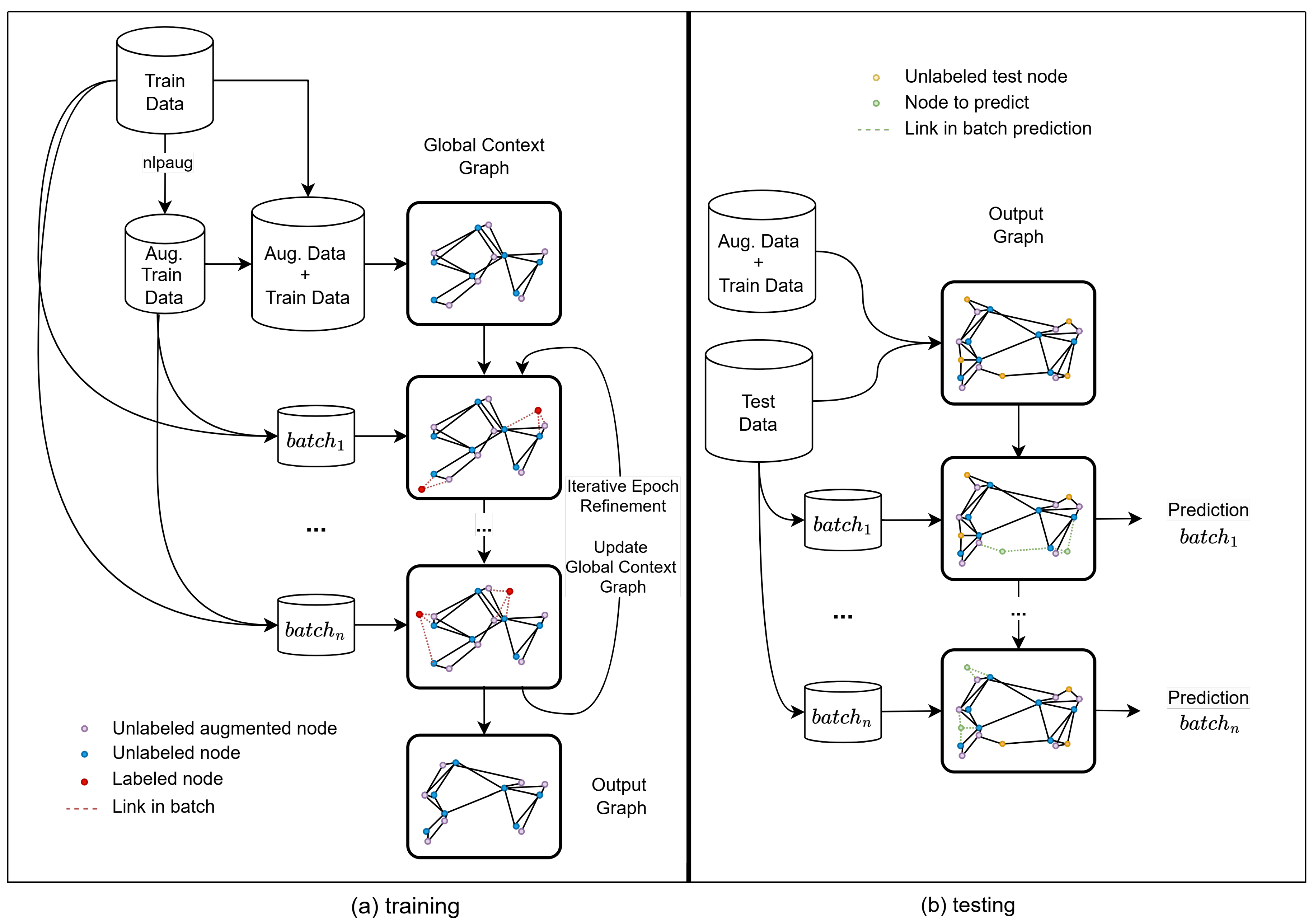
Figure 4.
Testing procedure of DynGraph-BERT: Label Propagation at Test Time
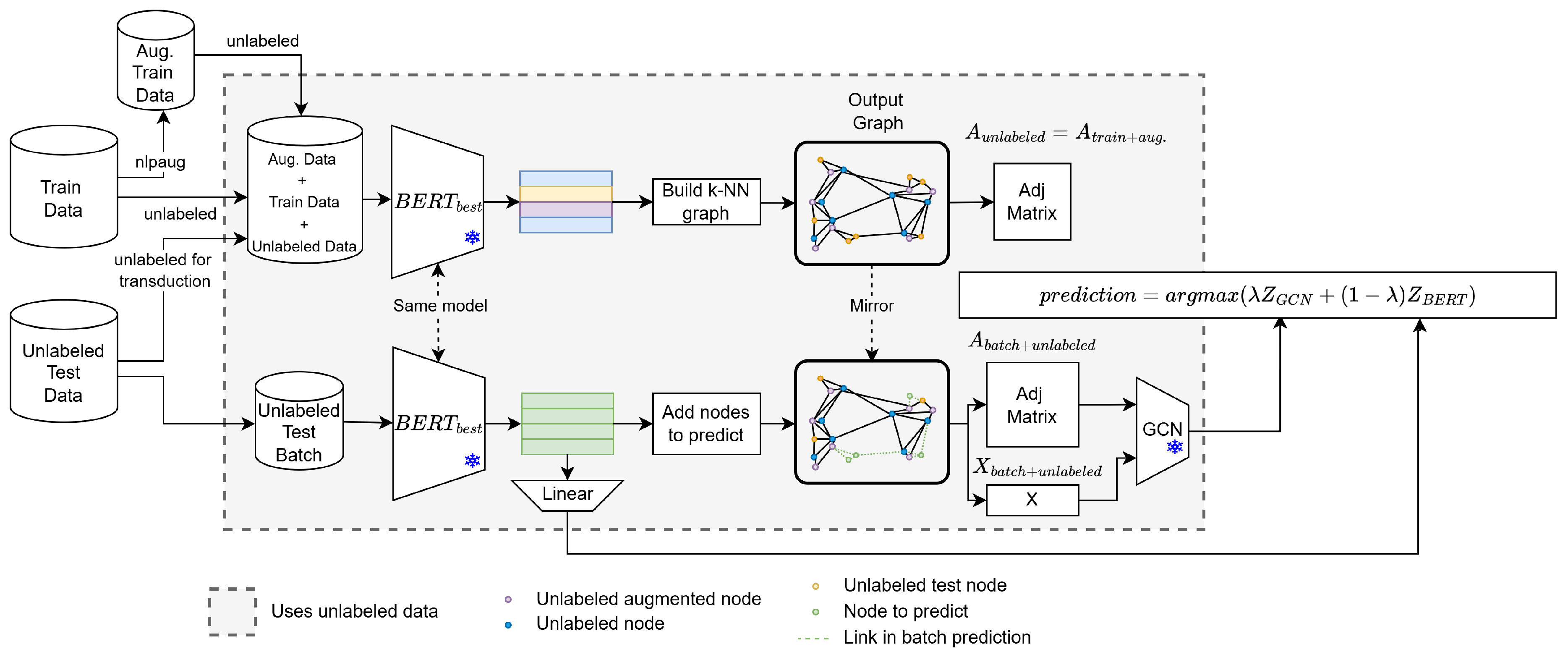
Figure 6.
Plots for ablation study. (a) Maximum number of neighbors for graph construction on the Snippets dataset. (b) Minimum similarity for graph construction on the Snippets dataset. (c) Variation of in the model’s loss function for the Ohsumed and AGNews datasets.
Figure 6.
Plots for ablation study. (a) Maximum number of neighbors for graph construction on the Snippets dataset. (b) Minimum similarity for graph construction on the Snippets dataset. (c) Variation of in the model’s loss function for the Ohsumed and AGNews datasets.
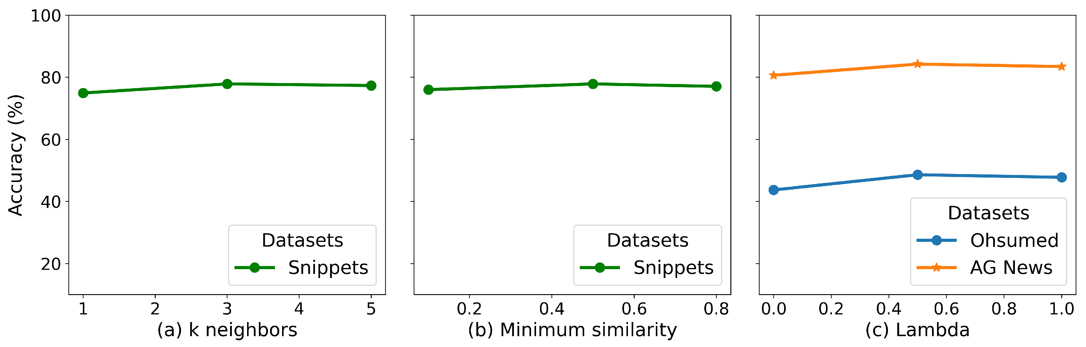
Table 1.
Examples of text generated using the augmentation techniques applied in DynGraph-BERT.
| Augmenter | Text |
|---|---|
| Original | The weather is beautiful today. |
| Swap | The climate is gorgeous today. |
| Omitting | The weather is today. |
| Typos | The weatger is biutyful today. |
| Change order | The weather is today beautiful. |
Table 2.
Summary statistics of datasets.
| Dataset | # Train | # Per Class | % | # Val | # Test | # Class | Avg. Len. |
|---|---|---|---|---|---|---|---|
| Ohsumed | 207 | 9 | 2.80 | 1000 | 6193 | 23 | 135.82 |
| R8 | 80 | 10 | 1.04 | 1000 | 6594 | 8 | 65.72 |
| AGNews | 40 | 10 | 0.50 | 1000 | 6960 | 4 | 26.85 |
| Snippets | 64 | 8 | 0.52 | 1000 | 11276 | 8 | 17.73 |
| DBLP | 120 | 20 | 0.50 | 1000 | 22880 | 6 | 8.51 |
Table 3.
Hyperparameters.
| Hyperparams | Value |
|---|---|
| hidden size | 256 |
| embedding dimension size | 768 (BERT) |
| aug. data | 2 |
| batch size | 16 |
| dropout | 0.66 |
| number of layers | 2 |
| epochs | 20 |
| learning rate BERT | 1e-5 |
| learning rate GNN | 1e-3 |
Disclaimer/Publisher’s Note: The statements, opinions and data contained in all publications are solely those of the individual author(s) and contributor(s) and not of MDPI and/or the editor(s). MDPI and/or the editor(s) disclaim responsibility for any injury to people or property resulting from any ideas, methods, instructions or products referred to in the content. |
© 2024 by the authors. Licensee MDPI, Basel, Switzerland. This article is an open access article distributed under the terms and conditions of the Creative Commons Attribution (CC BY) license (http://creativecommons.org/licenses/by/4.0/).
Copyright: This open access article is published under a Creative Commons CC BY 4.0 license, which permit the free download, distribution, and reuse, provided that the author and preprint are cited in any reuse.


