
Submitted:
02 December 2024
Posted:
09 December 2024
You are already at the latest version
Abstract
Presents a proof-of-concept version of a versatile PQ analyser for tracking the voltage supply in industrial and residential sectors. Implements 2D higher-order statistics to assess power fluctuations based on the sinusoidal waveform. Thus, beyond the second-order parameters and permissible deviations regulated by the norm EN 50160, the two-dimensional traces and probability density functions, along with a previously studied differential index manage to identify different states of the electrical grid. Waveforms have been measured in the point of common coupling of a public building. Being suitable for analysing both power quality and reliability, results convey that incorporating skewness and kurtosis to reports enhance the characterization, as well as extract the customers' supply behavior under normal and anomalous operations, considering both time and location patterns. The principle fosters a robust performance in real-life campaigns, which demonstrate the good behaviour in site characterization. The method is considered as a probabilistic approach for the risk assessment.
Keywords:
energy data
; higher-order statistics
; measurement instrument
; network voltage status
; Power Quality tracking
1. Introduction
Over the last ten years, renewables in the energy mix has grown by 10 %, mainly due to the greater number of countries that encourage their use to align with European environmental directives [1]. However, due to the penetration (in capacity and distribution), and the random and disperse nature, the electrical network has been affected to such an extent that the assessment of the supply has become a challenge that requires often tailor-made measurement solutions. Indeed, the intermittence (also deregulated connections) and non-linearities (based on power electronic devices) have given rise to new and hybrid types of disturbances that damage the more sensitive electric loads, such us IoT sensors, adjustable-speed drives and computers [2,3,4,5,6,7,8].
In this frame, the confluence of statistical signal processing, IoT instrumentation and measurement techniques, pursues the following fulfilments:
- Characterisation of the power system. The new trends in instrumentation campaigns lie in the strategic hypothesis that on-demand monitoring pursues better quality assurance and energy efficiency, and consequently reduces the carbon footprint [4].
- Collecting energy usage data. Handling massive information (big data), specially from the burgeoning digitization of the modern industry sector (e.g., the so-called industries 4.0 and the human-centred 5.0).
- Eliminating the redundant information in order to save memory [11].
- Detection of new PQ events. Characterisation of hybrid disturbances has fostered the development of new estimators beyond the traditional Gaussian-based (second-order).
So far these guidelines had not been considered, because PQ has been associated to high degree of expertise. They are outlined hereinafter. Firstly, the design of emerging measurement equipment along with myriads of new strategies pursue the subjacent elaboration of benchmarks to take a closer look at the daily industrial practice via a continuous monitoring; allowing companies to compare data from other companies who share information as well. This provides valuable context, helping to set meaningful targets; thus gaining insight into trends that occur across each company, and finding out how they are performing as compared to the competitors.
Secondly, the scalability in space and time stands out. Indeed, grid performance analysis conveys the characterization of multiple locations, which produces huge volumes of data that require proper organization, i.e., big data handling. This in turn is built on the elimination of redundant and erroneous information and the formulation of ad hoc indicators that bring together the significance of the measurements adapted to the requirements demanded by the customer, i.e., a more realistic network status [10,12,13]. Until now, measurement campaigns had been based mostly on instrumentation and strategies designed under the IEC 61000-4-30 standard [14]; but also, in recent years, in a complementary way, the reporting levels are increasingly inspired by the so-called and well-known PQ triangle [15], a context in which the scalability term appears. The goal essentially consists of extracting precise information regarding the state of the network and the electrical disturbances that most likely prevail in the site under test, carrying out an ad hoc characterization of the energy system. The analysis window (temporal scalability) and zone averaging (spatial scalability) are used together to offer a clear view of the PQ evolution. This strategy ensures an efficient data management that in turn improves the repeatability of the measurements and favours their traceability [16].
Third, in order to put the aforementioned objectives into practice, network operational data must be refined, as a result of a feature extraction stage that guarantees fidelity (e.g. eliminating redundancy and outliers). This must occur not only in abnormal conditions but also during rated regime [17,18]. In other words, measurement campaigns must produce reliable data that reduce the uncertainty of subsequent actions, derived from the industrial process control [10].
In fourth place, there is a need for targeting hybrid disturbances, especially continuous events [8,19,20]. In literature, the real-time surveillance is not improved enough to achieve these ending [21], and examples on the characterization of multiple events and network statuses in long term monitoring cannot be found frequently, or are very limited [22]. Thus, the current technology and measurement strategies lack a generalized approach to the problem that handles multiple events within a network status operation [22,23]. The present work implements a solution to track hybrid PQ events based in 2D-trajectories of the indices.
In this frame, new trends in measurement solutions manage information by converting big data from each smart meter into parameters of a probability distribution, and then calculating the distance to profiles. These actions transform each time-series (e.g., demand data) into a two-dimensional (2D) scatter plot [17], becoming more traceable and understandable for both customers and suppliers. In this line, this work goes one step forward and uses diagrams of higher-order statistics (2D-HOS) that characterize the voltage, compresses the time-domain measurements and, cycle-to-cycle, computes the evolution of the 2D waveform vector. It contributes to the main PQ goals, including data compression, scalable indices and continuous monitoring. In addition, this strategy differs from the conventional which are only based on the second-order magnitudes. In fact, complementary techniques (e.g., wavelets) have provided hopeful results in shape identifications, but they are still far susceptible to noise and the computation cost is high, [19].
This paper is a logical continuation of the works in [10,24] and [25] and presents a HOS-based non-intrusive measurement solution (physical distributed measurement) conceived to monitor the states of the electrical supply voltage at any point in the network, whether upstream or downstream. Being noise immune and focusing on the waveform, the proposed indicators help characterize the point under test and inform when the surveyed parameters fall outside the normal operating conditions and surpass the contractual thresholds. Additionally, two acquisition devices have been proposed in order to show its design flexibility.
From the point of view of technology maturity, the prototype successfully demonstrates operation in a real environment, which is indicative of TRL1 level #7.
The rest of the paper is organized as follows. Section 2 exposes the mathematical foundations of the measurement strategy, along with the comparison with the most similar and relevant existing methods (also performed in the present introduction). The measurement activities framework and the instrument design (hardware and software) are presented in Section 3. Then, Section 4 presents the results and discussion along with the instrument performance, browsing through the panels and tabs, in order to show its potential, and practice. Finally, Section 5 summarises valuable theses derived from the practical performance and the visual results.
2. Continuous Monitoring Based on HOS
2.1. Second-Order vs. HOS-Based PQ Indices
The mathematical foundations lie on the hypothesis that HOS-based indices are far sensitive to shape parameters. So far neither gathered nor considered within current norms and standards, this potential is used in the extraction of the voltage supply features. Traditionally, the formers have to do with the so-called second-order regulated measurements, such as the or the THD (Total Harmonic Distortion), in the time and frequency domains, respectively [26]. However, literature has revealed the need for new tools in order to look beyond the power change [10,27].
Background research has also elicited the need for tracking continuously the power-line waveform. Indeed, the variance detects changes in the amplitude as a result of power changes, which is indicative of sags and swells [18]. The skewness can be positive or negative depending on the sizes of the right and left tails of the probability density function (PDF). If the left (right) is more evident than the right (left) the skewness is negative (positive). Non-symmetry in electrical events indicates the half-cycle in which the deviation takes place. Therefore, skewness is capable of detecting transients and the non-symmetry of the starting and ending parts of the events, such as sags and swells. The kurtosis characterizes the tails of the statistical distribution. In the context of voltage waveforms, the flatter the top and down regions, the lower the kurtosis will be [18].
Regarding feature extraction, the importance lies in the previous pre-processing that guarantees maximum probability of detecting not only the events but also the network behaviour under normal operation, which is the main goal in this paper. This is crucial for the power recognition systems [17,18] in terms of statistical behaviour. Also, the PQ campaigns must produce reliable data that accomplish the metrological requirements under a Bayesian optics and reduce the uncertainty in the process control [10]. In literature, the real-time events detection and characterization are not improved [21] and examples on the characterization of multiple events in real-time monitoring cannot be found frequently [22]. Thus, the current PQ technology lacks a generalized approach to the problem that handles all different events, i.e., single and multiple events [22,23]. Other signal processing tools such as wavelets [19] and estimators based on echo state networks [20,28] have provided good results in shape identifications, but the noise influence is still noticeable. Also, as suggested before, there is a need for targeting new types of disturbances, more specifically, continuous events [19,20]. In this sense reference [28] introduces statistical similarity metrics, using successive cycles of the signal and detecting outliers. All in all, bearing this in mind, the technique proposed in this paper introduces HOS, which provide noise immunity.
Table 1 is thought for comparing HOS’s performance with that of the second-order ones. Specifically, variance (proportional to ) and crest factor, CF2, are compared with skewness and kurtosis, which are third and fourth-order statistics, respectively. Being the first the asymmetry coefficient and the second the tailedness coefficient of the statistical distributions of the signal amplitudes, these indicators constitute an important complement to the CF to confirm the presence of an anomalous operating state. The analysis is conducted according to different time domain voltage supply signals that lose their symmetry, their sinusoidal character or both: Symm-Sinusoidal, Symm-NonSinusoid, Symm-NonSinusoid, NonSymm-NonSinusoid, as for example in [27,28,29].
As compared to classical indicators, the calculation of the and the variance are based on squaring the signal, so results are almost identical. Therefore, any change detected by the first is targeted by the second. With respect to the CF, as it is the ratio of the maximum point to the effective value, and can be affected by noise or small impulses in the peaks. However, kurtosis is an estimator based on the distribution of points relative to the mean, indicating whether they are more concentrated or dispersed, and is less sensitive to the variation of a point on the ridges. Finally, traditional indicators work under the premise that the wave is symmetrical, since it is a premise of the normal operation. However, during transients, specific or temporary asymmetries may occur, which are detected by the skewness.
Table 1 includes the behaviour of the differential PQ index (variance, skewness and kurtosis), based on previous results [25,27], which take into account the differences between the ideal and real variance, skewness and kurtosis, in absolute terms, respectively. This index is recalled by Eq. 1:
where is the measurement time interval, the i-th cycle within , M is the number of periods within the time interval , is the j-th sample statistic associated with the i-th period (e.g., , , ), and is the expected j-th statistic. Based on the former definitions and strategy, hereinafter the subsequent design of the virtual instrument (VI) is explained. The solution to monitor the network voltage will be based on graphs with higher-order statistical indicators and a numerical index that in the case of an ideal voltage supply is zero, and deviations from this value show a change of state in the network.
2.2. Mathematical Foundations of HOS
Originally, HOS were proposed to infer new characteristics associated with blurred time-series in predominant Gaussian background [2]. Within the specific context of PQ detection, the targeted electrical disturbance is considered non-Gaussian, while the floor is assumed to be a stationary Gaussian or a symmetrically distributed signal.
If the focus is put on the waveform, HOS provide new information, not issued by the second-order measurements (e.g., power measurements). Indeed two signals can be valued with the same and exhibit different time-patterns [31].
In the context of voltage quality, HOS are even more suitable since they characterise the waveform itself, thus increasing the probability of discriminating among types of disturbances, if the analysis window is small; or amidst operating states of the electrical network, in case of focusing on longer observation intervals, such as in reliability studies. This can only be discriminated using statistics of higher orders, as described by the cumulants, which are defined hereinafter.
Let x(t) be an rth-order stationary real-valued random process (e.g., instantaneous voltage line supply). The rth-order statistical cumulant is defined as the joint self-correlation of the random variables , , , ..., , where , ,...,, are time shifts multiples of the sampling period, ; i.e., =, with j∈. The first time shift, =0, corresponds to the original signal, without time shifting. The most common cases of the cumulants are the second-, third- and fourth-order; for instance for the second, and third order we have:
For a process without mean or time shift, Eq. 2 is particularized to the case of variance, skewness. Since HOS have succeeded in other fields (e.g., vibration mechanics, acoustic emission detection) they are suitable for the new power grid scenario. Indeed, this tool contributes significantly to the classification of electrical disturbances since it addresses not only the instantaneous power, but also those associated with waveform [27,31]. This confers HOS with suitable characteristics in order to analyse the new type of PQ disturbances. Also, depending on the cumulants’ orders, the observed interdependency will lead to specific states of the system under test and will enable the inference of some properties related to the system behaviour.
The strategy consists of calculating three statistics: the variance, the skewness and the kurtosis. In the case of the ideal sinusoidal supply voltage (50 Hz), this triplet is referred as (0.5, 0.0, 1.5), respectively, assumed as the ideal steady-state from which to measure deviations [25]. In practice, the absolute deviation index is not null, since the power line is not ideal neither in frequency nor in shape. Likewise, by gathering the measurements of each record in three statistical parameters, the memory savings are notable (time compression), which indicates that this index is suitable for dealing with big data.
3. Virtual Instrument: Context and Design
3.1. General Measurement Framework
The general framework is deployed in the conceptual diagram of Figure 1. The virtual instrument (VI) is thought for providing valuable insight into the PQ big data trend that has been previously acquired and compressed in the time domain. Data can be further used in a number of applications, ranging from forecasting to PQ and energy management benchmark.
Measurements were conducted at the University of Cádiz, Spain, during a six-week campaign. The goal is to monitor the 50-Hz LV at a 25 kHz (i.e., 500 samples per cycle) sampling rate in order to test the shape of the voltage supply signal.
3.2. Description of the Instrument Hardware
Figure 2 shows the two versions of the measurement chain, ranging from the physical variable (the voltage line signal) to the laptop computer, which emulates the control panel at the consumer’s side. This single-phase version of the instrument is made up of the following elements. A voltage differential probe model HZ-115 (Hameg Instruments) is connected to the voltage DAQ module card, model NI-9215, which is hosted in the bus-energized chassis NI-cDAQ-9191. The supply voltage is attenuated by the probe and then conditioned to a range of ±10 V.
The Figure 3 shows the real-life differential probe (3a), used in the first version, and the NI c-DAQ chassis (3b) chosen for the instrument design. The probe has an overall accuracy of ±0.5% and it is designed for measuring nominal voltages from ±10 to ±500 V. The DAQ module NI-9215 has four input channels, a resolution of 16 bits per channel and a maximum sampling frequency of 100 kS/s/channel. The input range is ±10 V, and also includes a NIST-traceable certification which allows time stamping. The chassis establishes the physical or wireless link between the laptop computer and the DAQ board.
The interest of the first version consists of showing off the design flexibility of the distributed instrumentation. Furthermore, in an advanced measurement chain, the differential probe is eliminated to improve ±0.5% gain accuracy, and to increase the sampling resolution up to 24 bits. In this case, the DAQ hardware is the voltage module, C series, NI-9225, 50 kSPs (data rate), 24 bits, 300 , instead of the pair HZ-115/NI-9215 (16 bits, 100 kSPs).
From this point in the paper onwards, the software is described by navigating through its different panels (interfaces) and showing the most significant results and capabilities.
3.3. Description of the Instrument Software
The software has been designed and implemented using the environment. The graphical user interface (GUI) for the VI is specially designed to separate the hardware control and data acquisition settings from the data displays and graphs, which in turn are designed to display the optimal spatial and temporal configuration, so that to extract and interpret the data. The GUI consists of five panels (or tips): two for acquisition and configuration set up (the core of the system), and three for statistical adjustments, called Acquisition, Config, HOS Fingerprint, HOS Histogram and Trajectories, respectively. In this sub-section the two first are introduced.
Two VIs work cooperatively. The main one includes the analysis, the core structure, as well as the following tabs: Config, HOS Fingerprint, HOS Histogram and Trajectories. On the other hand, the sub-VI responsible for acquiring data, can be seen in the Acquisition tab, and accumulates the data until the main VI is ready to analyze. Data should be read from the acquisition card as soon as available (the data block required, e.g. 1-second length), to prevent the memory card from saturating and the acquisition being interrupted. Two independent data reception systems ensure that this will not happen; in fact, the two programs communicate each other through shared variables.
Figure 4 shows the Acquisition tab. Here the reception of the data is surveyed, indicating the card and the channel in DAQmx Physical Channel (s), the Sampling Frequency, , and the Duration (s) of each measurement. Continuous measurements are carried out without interruption. The maximum number of signals to be accumulated (waiting to be analyzed) is previously indicated to avoid overflowing memory. We will be able to see the status of the analysis queue (signals waiting), the acquisition status, and if an error occurs, the reason why. To begin, the user presses "Start ACQ". We have the option to stop the acquisition in case we want to modify the parameters ("Stop ACQ") and continue after an error, as well as eliminate the signals pending (Flush Queue).
Figure 5 illustrates the Configuration panel. It establishes the analysis setup, i.e., the network frequency, nominal values and limits, as well as the size of the persistence-type graphs. This configuration predefines the 2D graphs, that appear in the following tab, and that in turn illustrates the subsequent fingerprints of the statistics, for the given selected refreshing time. A case with five sub-graphs is indicated in Figure 6 and a situation with four is depicted in Figure 7. Thus, all subsequent stages consider different time horizons, which are defined here, indicating a numerical and a time unit. The case represented in in Figure 7 corresponds to the last two hours, 1 h, 1 min and 10 s, respectively. On the right-hand side area, the names of the graphs are configured, using formatted string wildcards.
The Figure 5 also shows a graph (bottom-right corner) thought to monitor the current acquisition of the 50-Hz grid voltage, whose amplitude is normalized before applying the statistical computing algorithms. The real voltage is indicated above, and it is used to normalize the input voltage and adjust the scale factor of the probe. Normalization allows the algorithm to extend its validity to any network under monitoring.
Aiming to provide the information generated, for each period (20 ms), the dimension of the data vector is . The algorithm calculates three statistics (N=3; variance, skewness and kurtosis) using a cycle-by-cycle sliding window, with no overlapping; each window computes 500 data, which are reduced to four parameters. In a subsequent stage, the values are subtracted to the ideal quantities, their absolute values calculated, and the final differences added to the resulting PQ index recalled in Eq. 1.
The next Section 4 presents the instrument’s behavior while describing the measurement campaign at the same time.
4. Virtual Instrument: Performance Results and Discussion
The instrument operates in real-time. It is preferred to show its performance within an offline description through the main panel overview, which is by the way one of its best functionalities, because it allows getting the most of big data depending on the analysis time window.
As a general observation of the measurement campaign, the daily PQ fluctuates depending on the day of the week, the hourly trend of the network, the energy usage during working or non-working hours. During the night, the PQ cycle-to-cycle can fluctuate between 0.01-0.02 values. During the morning the deviation increases reaching a maximum of 0.04 during the noon. Also, between 13H00-16H00 there is a drop because this is the lunch hour. A second increase of the index occurs in the evening schedule, since the University opens until 22H00, the closing time. Finally, during midnight the PQ decreases again, recovering the minimum.
Indeed, 2D graphs available in the different panels allow visualizing such behaviour by emphasizing the areas of signal persistence throughout the hours, days and weeks. Hereinafter the three tabs that allows graphical representations are exposed: the HOS fingerprint, the HOS histograms panels, and the HOS trajectory panels, respectively.
4.1. The HOS Fingerprint Panel: Energy Traces
The tab corresponding to the layout of the footprint, or voltage trace, the HOS fingerprint panel, allows to monitor the network status. In this example, the focus is put on the variance vs. kurtosis time-scaled traces. Two design versions of the panel have been selected, depicted in Figure 6 and Figure 7, respectively, aiming to show different network status.
A direct observation is that the waveform is far from being ideal, as all the measurements in the colour maps for both figures exhibit a dispersion or bias with respect to the theoretical target center, the solid cross. From top to bottom and left to right, the different graphs show the HOS from the highest to the lowest scale. The color map represents the cumulative probability traces.
On the other hand, in the top-right part of each sub-trace the user is informed about the PQ index value that aggregates all the points that take part in the associated 2D graph below; also, the instruments is capable of selecting the outliers of the dispersion cloud (top right side in each sub-graph). If the waveform goes out of bounds, the outliers counter is increased. The brightest spots correspond to the most probable status of the voltage supply. The next one put the focus on a day within the week, where different intensity zones start to appear, denoting different status of the energy and voltage deviations. This fact is confirmed in the hourly plot.
The first representation in Figure 6 gathers all the data in one-week campaign (upper-left subgraph). Then, they are down-scaled to one day, one hour, 10 min and 10 s, respectively. The solid cross of each sub-graph corresponds to the ideal value of the pair variance=0.5; kurtosis=1.5. While these first three 2D graphs account for the reliability of the voltage supply, the two graphs below are thought to inform about PQ, subsequently looking at shorter intervals, and looking for PQ events, as stated in the norm IEC 61000-4-30.
Figure 6.
Panel implementing the energy trace for the variance-kurtosis: one example of the energy trace from 1 week to 10 s-window; previously set in the Configuration panel.
Figure 6.
Panel implementing the energy trace for the variance-kurtosis: one example of the energy trace from 1 week to 10 s-window; previously set in the Configuration panel.
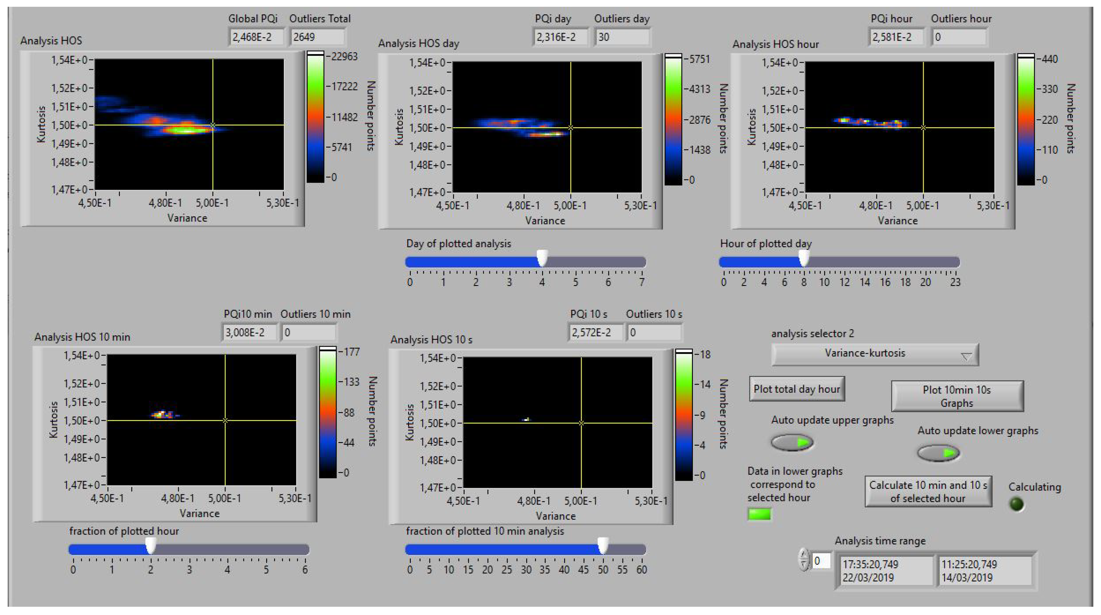
Figure 7 is another version of the fingerprint panel which contains four sub-graphs and incorporates the clusters’ center, with a dashed cross. This version is suitable for establishing the distance from the real centroid to the ideal center, according to the Euclidean metrics.
Figure 7.
Panel that implements the energy trace for the variance-kurtosis pairs. The centroid of the clusters (dashed cross) established the bias from the ideal operation state of the electrical network (continuous cross). The hourly graph shows a more stable network than in Figure 6.
Figure 7.
Panel that implements the energy trace for the variance-kurtosis pairs. The centroid of the clusters (dashed cross) established the bias from the ideal operation state of the electrical network (continuous cross). The hourly graph shows a more stable network than in Figure 6.
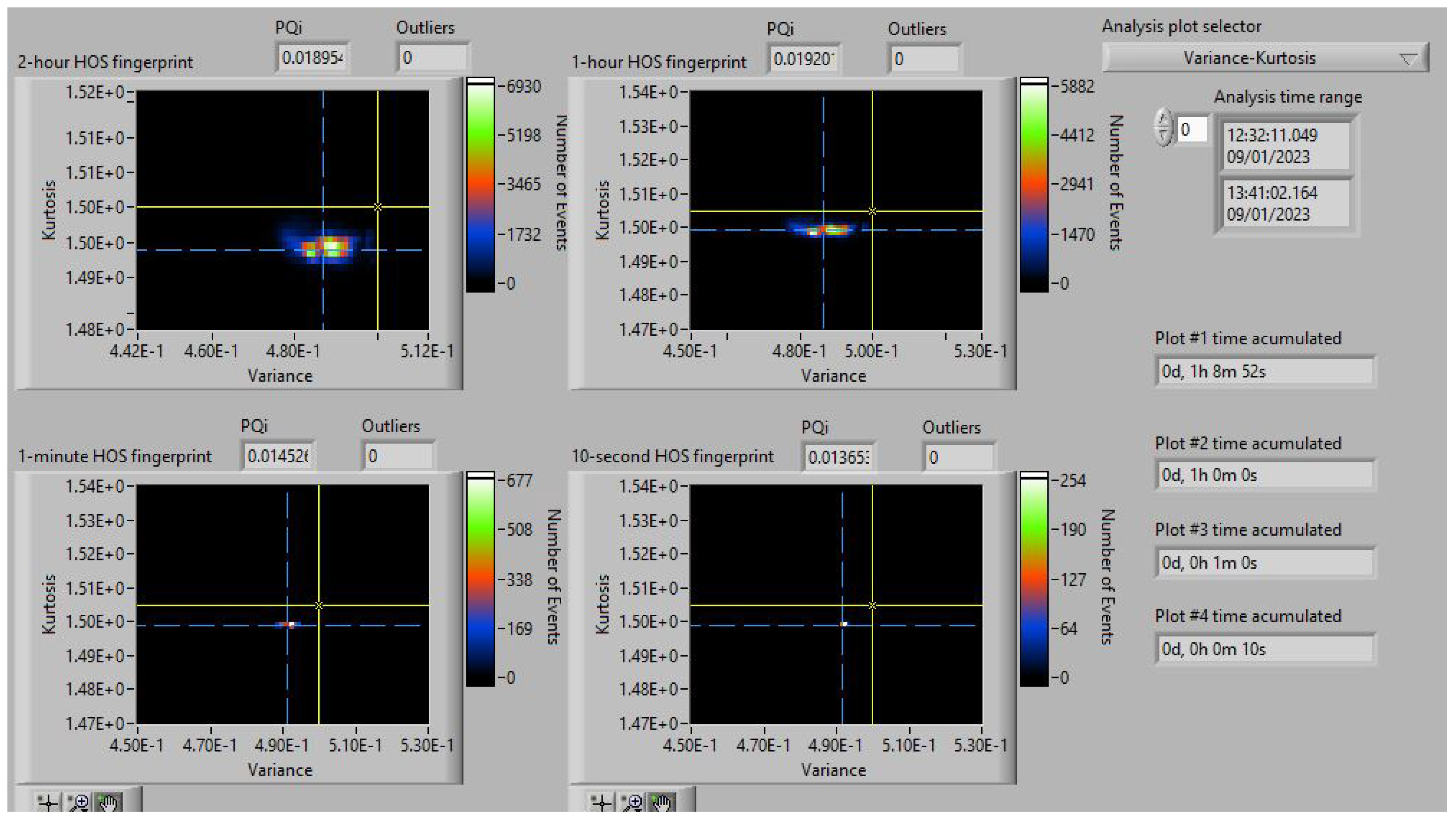
Both figures illustrate different experimental behaviors. For example, comparing the two hourly sub-graphs greater network instability is observed in Figure 7 than in Figure 6. Being the yellow centroid the reference, in the first the variance ranges from 0.465 to 0.485, while the second presents a far smaller (negligible) dispersion around the clusters’ centroid and the dashed cross (the global centroid).
The following programming flow diagram, Figure 8, illustrates the procedure conceived to obtain the two-dimensional plot of the voltage supply quality, the HOS-footprint or energy trace, which explains the state of the electrical network. The analysis, as in the previous case, is arranged and performed in pairs, i.e., variance-kurtosis, variance-skewness or kurtosis-skewness.
As seen in Figure 8 firstly, the software initialises a matrix (zero) with the dimension of the representation, and then it reads each pair of HOS values. This two-dimensional array of zeroes will constitute the fingerprint storage later on. First, the HOS values are compared with the extremes, assigned by the user, that are considered as limit network-condition status. If any of the two data variables of the pair is out of range (greater than the maximum or less than the minimum indicated for that axis), the point is considered as outlier, the outlier counter is incremented, and end up with this pair of values. Otherwise, if both data in the analysed pair fall within range, an integer position among max and min is assigned for each one, with an integer division by the increment (max-min divided by the fingerprint vector dimension). Thus, the increment is calculated as the maximum minus the minimum, divided by the number of points on the axis. To obtain the value, the minimum of the axis is subtracted from the current HOS value, and the result is divided by the increment, leaving with the integer part of the division. The same is done for both axes and will obtain the pair of statistics to which the analyzed signal cycle corresponds, and finally add 1 to it. After that the next pair of HOS is considered, i.e., the position indicated by both indexes, related to division of both HOS, is incremented by one.
When all HOS variables are analysed, a two-dimensional representation is obtained, giving rise to a colourful map, in which different colours are seen depending on the frequency with which the data is repeated, as can be seen in the colour bars in the Figure 6 and in Figure 7. In this panel, the area in which data is located is also marked by means of the cursors (continuous axes) to comply with the power quality requirements, as can be seen in both.
4.2. The HOS Histograms Panel
Figure 9 shows the panel of the instrument corresponding to the histograms of the variance, skewness and kurtosis, respectively, obtained according to different averaging times, i.e. 1 hour, 1 minute and 10 seconds, respectively. Since it is a real signal that is being monitored, these histograms are not centred on the ideal values: 0.5, 0.0 and 1.5 for variance, skewness and kurtosis, respectively. In all of them, it is worth remarking that the longer the averaging time (time interval window), the more accurate the measurement of the most probable value, since the fluctuating statistics are compensated.
Hereinafter the trajectory panel is presented.
4.3. The HOS Trajectory Panel
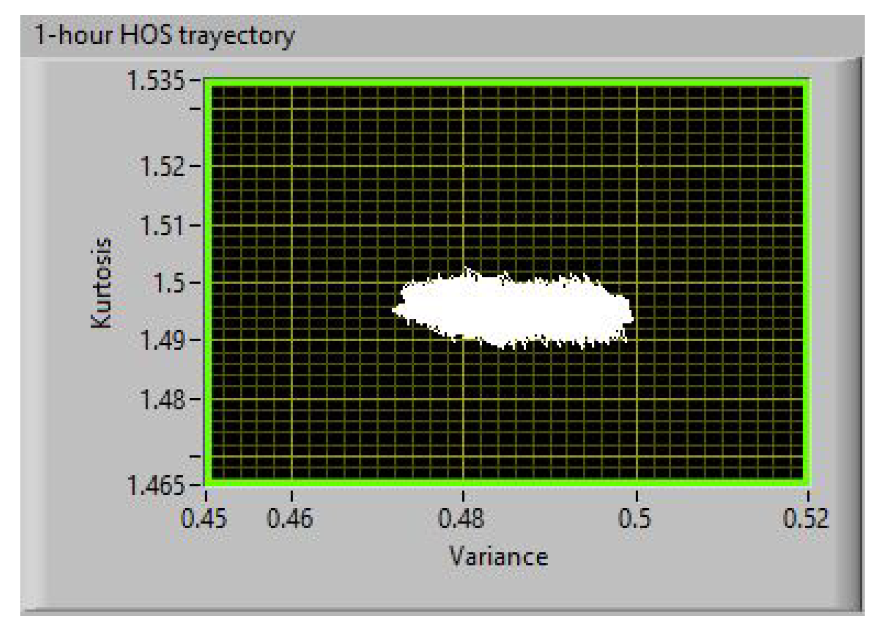
The panel shows the trajectory following a two-dimensional dynamic evolution of a pair of statistics previously selected by the user among those studied in the time-domain. These statistics are calculated with a time resolution of one network signal cycle (20 ms), which is the minimum needed to carry out operations. That is, each cycle can have a triplet or variance-skewness-kurtosis vector. Thus, for example, Fig. shows the evolution of the kurtosis (Stat. #2) vs. the variance (Stat. #1). The monitored statistics in this figure have ideal values at the coordinate point (kurtosis=1.5, variance=0.5); and a rectangular zone of error margin has been represented with ranges [0.45-0.52] for the variance and [1.465-1.535] for the kurtosis, respectively, corresponding to the maximum values observed during normal supply day. The trajectory, with a total duration of one hour, is given by the cloud of points, whose centroid is separated from the previous idyllic point (var=0.5, kur=1.5), and which corresponds to the situation of perfect voltage supply. In this case, the supply holds steady within the tolerance region established according to the empirical criteria previously outlined.
Figure 10.
Variance vs. kurtosis 1-hour trajectory.
The programming code shown in Figure 11 is a section designed to implement the graph for the trajectory. Thus, it takes the vectors containing the statistics in the order in which they have been calculated, and later adds the quadrangular area that delimits the validity limits of the correct supply, as a second plot. The union of the two plots is done in the "bundle" type element, and the graphic representations are done in the "XY Graph" graphic -type elements.
The virtual sub-instrument block named Trajectory from HOS, shown in Figure 11 and whose "guts" (programming code) are shown in Figure 12 builds the higher-order statistics vector transferred to the graphs.
The 3D-vector coordinates are the higher-order statistics, where N corresponds to the number of voltage cycles that are analysed, calculating the variance-skewness-kurtosis triplet for each cycle. The selector in Figure 12 allows selecting the pair of statistics that will be represented. To do this, it receives a pair of indices, one for each axis of the 2D diagram; each index refers to a vector that contains all the values of its statistic measured in the selected time interval. These vectors are the inputs to the "XY Graph" building blocks of object-oriented programming. In this process lies the idea that the lowest temporal resolution used corresponds to one signal cycle.
The measurement system developed was tested in the facilities of a public building of the university, being able to detect deviations in 10-second traces of 3.9 % in variance and 0.6 % in kurtosis, as it is shown in Figure 7.
5. Conclusions
This paper summarizes the performance of a HOS-based virtual instrument that analyses big data for the evaluation of PQ. With new functions, the developed VI provides specific information that allows better tracking of domestic and industrial PQ. Taking the primary voltage measurements, it further calculates the statistics and maps the compressed parameter into 2D traces. Aggregating cycle-over-cycle, this visualization tool establishes the quality regions that characterize the behaviour of the energy system. Two possible hardware solutions have been shown.
As the HOS account for the waveform rather than for the power fluctuations, the instrument is capable of detecting hidden features in long term measurement campaigns, which are more in the smart grid framework.
In order to develop the site characterization through the PQ features, the time-series can be scaled to different averaged windows. Based on the authors’ experience, skewness can be useful in strategies more focused on short-duration windows and consequently thought to event detection strategies.
The VI developed in this work allows, in the first place, observing the energy bias in the analysed point of the network, with respect to the ideal characteristics that should meet. Also, the company can conduct inspections using a variable time window. In this way, different periods of the day associated with different energy qualities can be observed, as well as being able to establish a trend pattern from which to make decisions related to energy management and efficiency.
Future work focuses on a twofold strategy. On the one hand, there is the implementation of the program using a more flexible language that consumes fewer resources than . On the other hand, within the framework of the national project, the monitoring of PV solar plants will be carried out at the point of delivery.
Author Contributions
J.J.G.D.R. conceived the idea, led the researh, and wrote and prepared the manuscript. J.J.G.D.R, O.F.O. and A.A.P. developed the theoretical indicators on which the measurement instrument is based. J.M.S.F. programmed all the algorithms in LabVIEW. M.J.E.G. and J.C.P.S. connected the hardware. All authors have read and agreed to the published version of the manuscript.
Funding
This research was funded by Spanish Ministry of Science.
Data Availability Statement
The original contributions presented in the study are included in the article, further inquiries can be directed to the corresponding author.
Acknowledgments
The authors express their gratitude to the Spanish Ministry of Science, Innovation and Universities for funding the project PID2019-108953RB-C21, entitled Strategies for Aggregated Generation of Photo-Voltaic Plants-Energy and Meteorological Data (SAGPV-EMOD).
Conflicts of Interest
The authors declare no conflicts of interest. The funders had no role in the design of the study; in the collection, analyses, or interpretation of data; in the writing of the manuscript; or in the decision to publish the results.
References
- (IEA), I.E.A. International Energy Agency - Renewables. https://www.iea.org/fuels-and-technologies/renewables, 2023. visited, July 27th, 2023.
- Florencias-Oliveros, O.; González-de-la Rosa, J.J.; Sierra-Fernández, J.M.; et. al.. Power Quality Measurement and Analysis Using Higher-Order Statistics: Understanding HOS contribution on the Smart(er) grid; Wiley-IEEE Press, 2022. 192 Pages.
- Florencias-Oliveros, O.; González-de-la Rosa, J.J.; Sierra-Fernández, J.M. Continuous and Non-Intrusive Energy Monitoring Challenge: Smart Choices in Difficult Situations. 2023 IEEE 13th International Workshop on Applied Measurements for Power Systems (AMPS), Proceedings; IEEE, , 2023; Vol. 1, pp. 1–6.
- Chung, I.Y.; Won, D.J.; Kim, J.M.; Ahn, S.J.; Moon, S.I. Development of a network-based power quality diagnosis system. Electric Power Systems Research 2007, 77, 1086–1094. [CrossRef]
- Pukhrem, S.; Basu, M.; Conlon, M.F. Probabilistic risk assessment of power quality variations and events under temporal and spatial characteristic of increased PV integration in low-voltage distribution networks. IEEE Transactions on Power Systems 2018, 33, 3246–3254. [CrossRef]
- Bollen, M.H.; Bahramirad, S.; Khodaei, A. Is there a place for power quality in the smart grid? 2014 16th International Conference on Harmonics and Quality of Power (ICHQP), 2014, pp. 713–717.
- Barros, J.; de Apraiz, M.; Diego, R.I. A virtual measurement instrument for electrical power quality analysis using wavelets. Measurement 2009, 42, 298–307. [CrossRef]
- Hyndman, R.J.; Liu, X.; Pinson, P. Visualizing Big Energy Data: Solutions for This Crucial Component of Data Analysis. IEEE Power and Energy Magazine 2018, 16, 18–25. doi:10.1109/MPE.2018.2801441. [CrossRef]
- Bollen, M.H.; Gu, I.Y. Signal Processing of Power Quality Disturbances; Wiley-IEEE Press, 2006. 888 pp., IEEE Press Series on Power and Energy Systems.
- Florencias-Oliveros, O.; González-de-la Rosa, J.J.; Agüera-Pérez, A.; Palomares-Salas, J.C. Power quality event dynamics characterization via 2D trajectories using deviations of higher-order statistics. Measurement 2018, 125, 350–359. [CrossRef]
- de Oliveira, R.A.; Bollen, M.H. Deep learning for power quality. Electric Power Systems Research 2023, 214, 108887. [CrossRef]
- Ömer Nezih Gerek.; Ece, D.G. Compression of power quality event data using 2D representation. Electric Power Systems Research 2008, 78, 1047–1052. [CrossRef]
- Bollen, M.; Castel, R.; Friedl, W.; Villa, F.; Baumann, P.; Esteves, J.; Larzeni, S.; Ström, L.; Beyer, Y.; Faias, S.; Trhulj, J. Guidelines for good practice on voltage quality monitoring. 22nd International Conference and Exhibition on Electricity Distribution (CIRED 2013), 2013, pp. 1–4.
- IEC, U.E. UNE-EN IEC 61000-4-30:2015+AMD1:2021. Electromagnetic compatibility (EMC) - Part 4-30: Testing and measurement techniques - Power quality measurement methods, 2015.
- Gordon, J.M.R.; Meyer, J.; Schegner, P. Design aspects for large PQ monitoring systems in future smart grids. 2011 IEEE Power and Energy Society General Meeting, 2011, pp. 1–8.
- Ribeiro, P.F.; Duque, C.A.; Ribeiro, P.M.; Cerqueira, A.S. Power Systems Signal Processing for Smart Grids; Wiley-IEEE Press, 2013. 448 pp.
- Maheswaran, D.; Selvaraj, V.; Manjaly, D.P. Power quality monitoring systems for future smart grids. 23nd International Conference and Exhibition on Electricity Distribution (CIRED 2015), Lyon, France,, 2015, pp. 1–5.
- Agüera-Pérez, A.; Palomares-Salas, J.C.; González-de-la Rosa, J.J.; Sierra-Fernández, J.M.; Ayora-Sedeño, D.; Moreno-Muñoz, A. Characterization of electrical sags and swells using higher-order statistical estimators. Measurement 2011, 44, 1453–1460. [CrossRef]
- Saini, M.K.; Kapoor, R. Classification of power quality events. A review. International Journal of Electrical Power and Energy Systems 2012, 43, 11–19. [CrossRef]
- Mahela, O.P.; Shaik, A.G.; Gupta, N. A critical review of detection and classification of power quality events. Renewable and Sustainable Energy Reviews 2015, 41, 495–505. [CrossRef]
- Duda, R.O.; Hart, P.E.; Stork, D.G. Pattern classification, 2nd ed.; Wiley-Interscience: New York, 2001.
- Pou, J.M.; Leblond, L. ISO / IEC guide 98-4: A copernican revolution for metrology. IEEE Instrumentation & Measurement Magazine 2018, 21, 6–10.
- Khokhar, S.; Mohd Zin, A.A.B.; Mokhtar, A.S.B.; Pesaran, M. A comprehensive overview on signal processing and artificial intelligence techniques applications in classification of power quality disturbances. Renewable and Sustainable Energy Reviews 2015, 51, 1650–1663. [CrossRef]
- Florencias-Oliveros, O.; Sierra-Fernández, J.M.; González-de-la Rosa, J.J.; Espinosa-Gavira, M.J.; Agüera-Pérez, A.; Palomares-Salas, J.C. Instrument for Power Quality monitoring using Higher-Order Statistics 2D planes. 2021 IEEE 11th International Workshop on Applied Measurements for Power Systems (AMPS), 2021, pp. 1–6.
- Florencias-Oliveros, O.; González-de-la Rosa, J.J.; Sierra-Fernandez, J.M.; Agüera-Pérez, A.; Espinosa-Gavira, M.J.; Palomares-Salas, J.C. Site Characterization Index for Continuous Power Quality Monitoring Based on Higher-order Statistics. Journal of Modern Power Systems and Clean Energy 2022, 10, 222–231. [CrossRef]
- IEC, U.E. UNE EN IEC 50160 2011/A1:2015, 2015.
- Florencias-Oliveros, O. Instrumental Techniques For Power Quality Monitoring, Ph.D. Dissertation; Vol. -, 2020.
- Deihimi, A.; Rahmani, A. Application of echo state networks for estimating voltage harmonic waveforms in power systems considering a photovoltaic system. IET Renewable Power Generation 2017, 11, 1688–1694.
- Rahmani, A.; Deihimi, A. Reduction of harmonic monitors and estimation of voltage harmonics in distribution networks using wavelet analysis and NARX. Electric Power Systems Research 2020, 178, 106046. [CrossRef]
- Florencias-Oliveros, O.; González-de-la Rosa, J.J.; Sierra-Fernández, J.M.; Espinosa-Gavira, M.J.; Agüera-Pérez, A.; Palomares-Salas, J.C., HOS Measurements in the Time Domain. In Power Quality Measurement and Analysis Using Higher-Order Statistics: Understanding HOS contribution on the Smart(er) grid; 2023; Vol. -, pp. 27–52.
- Florencias-Oliveros, O.; González-de-la Rosa, J.J.; Agüera-Perez, A.; Palomares-Salas, J.C. Reliability Monitoring Based on Higher-Order Statistics: A Scalable Proposal for the Smart Grid. Energies 2019, 12. [CrossRef]
- de-la Rosa, J.J.G.; Sierra-Fernández, J.M.; Agëera-Pérez, A.; Palomares-Salas, J.C.; noz, A.M.M. An application of the spectral kurtosis to characterize power quality events. International Journal of Electrical Power and Energy Systems 2013, 49, 386–398. [CrossRef]
| 1 | Technology Readiness Level (TRLS) |
| 2 | Ratio between the maximum peak level and its effective value during a predetermined time. |
Figure 1.
Conceptual diagram that shows the location of the virtual instrument (PQA) in the electrical network and the types of measurements that can be carried out. The variance-vs.-kurtosis graphs indicate the state of the network for different time windows.
Figure 1.
Conceptual diagram that shows the location of the virtual instrument (PQA) in the electrical network and the types of measurements that can be carried out. The variance-vs.-kurtosis graphs indicate the state of the network for different time windows.
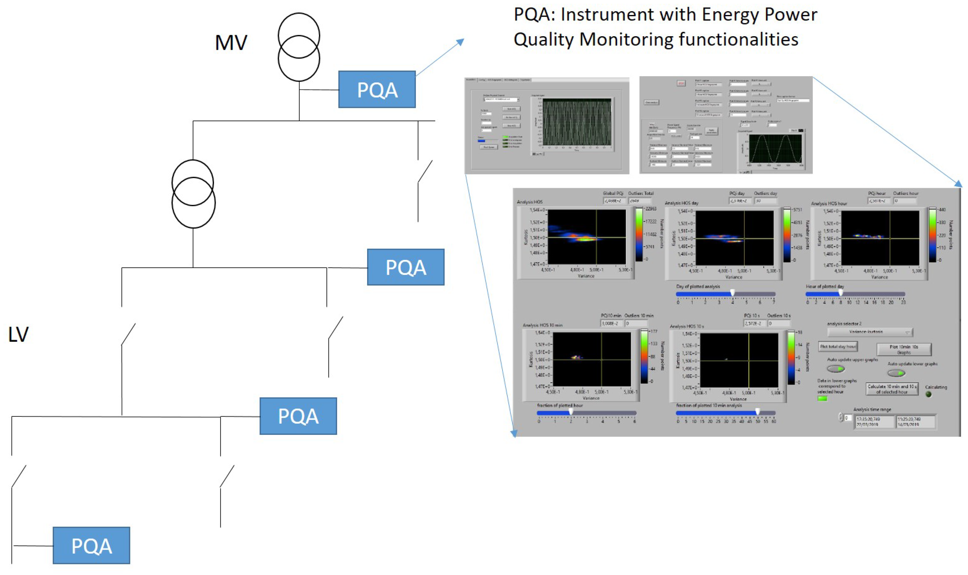
Figure 2.
Two versions for the measurement chain. The set is connected via Ethernet to a laptop computer in which a -based program performs the continuous analysis.
Figure 2.
Two versions for the measurement chain. The set is connected via Ethernet to a laptop computer in which a -based program performs the continuous analysis.
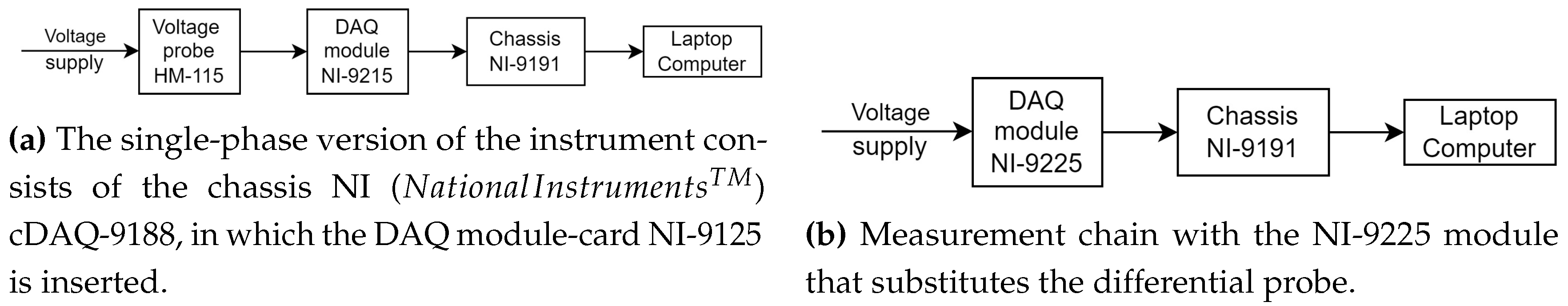
Figure 3.
Differential probe (a), and chassis (b) that hosts the DAQ card model NI-9215.
Figure 4.
Acquisition panel of the VI, where the user start or interrupt the acquisition.
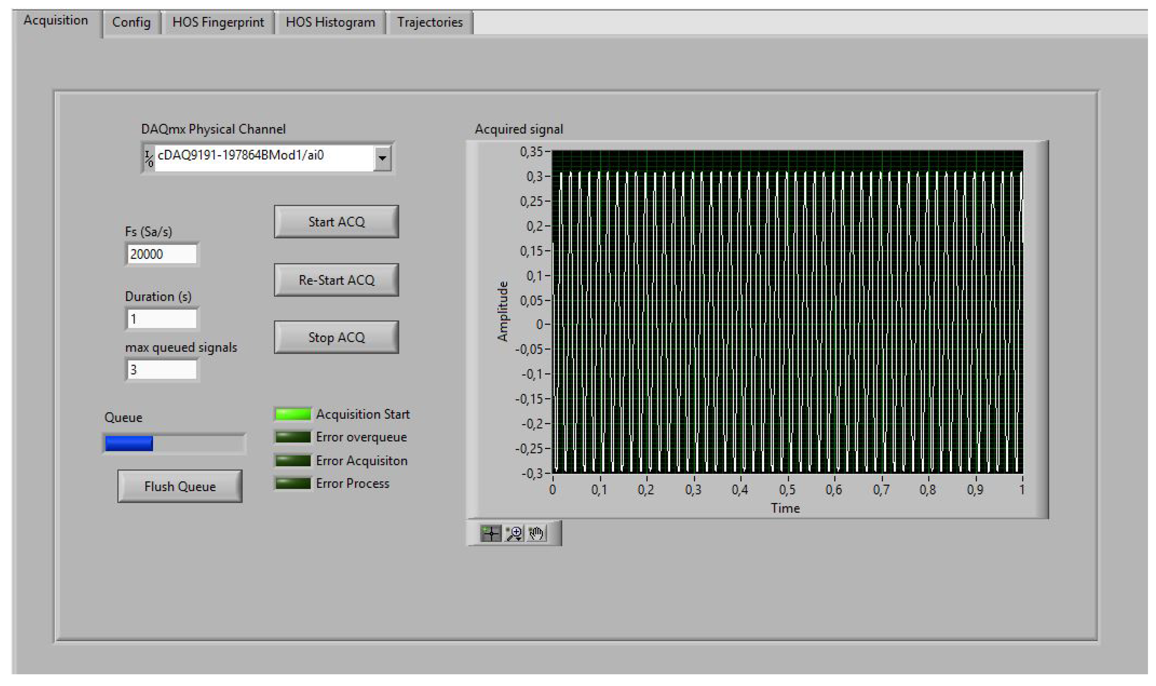
Figure 5.
Configuration panel of the VI, where the user can set: the ideal values of the statistics and the range, and the time to be accumulated in the 2D-plots.
Figure 5.
Configuration panel of the VI, where the user can set: the ideal values of the statistics and the range, and the time to be accumulated in the 2D-plots.
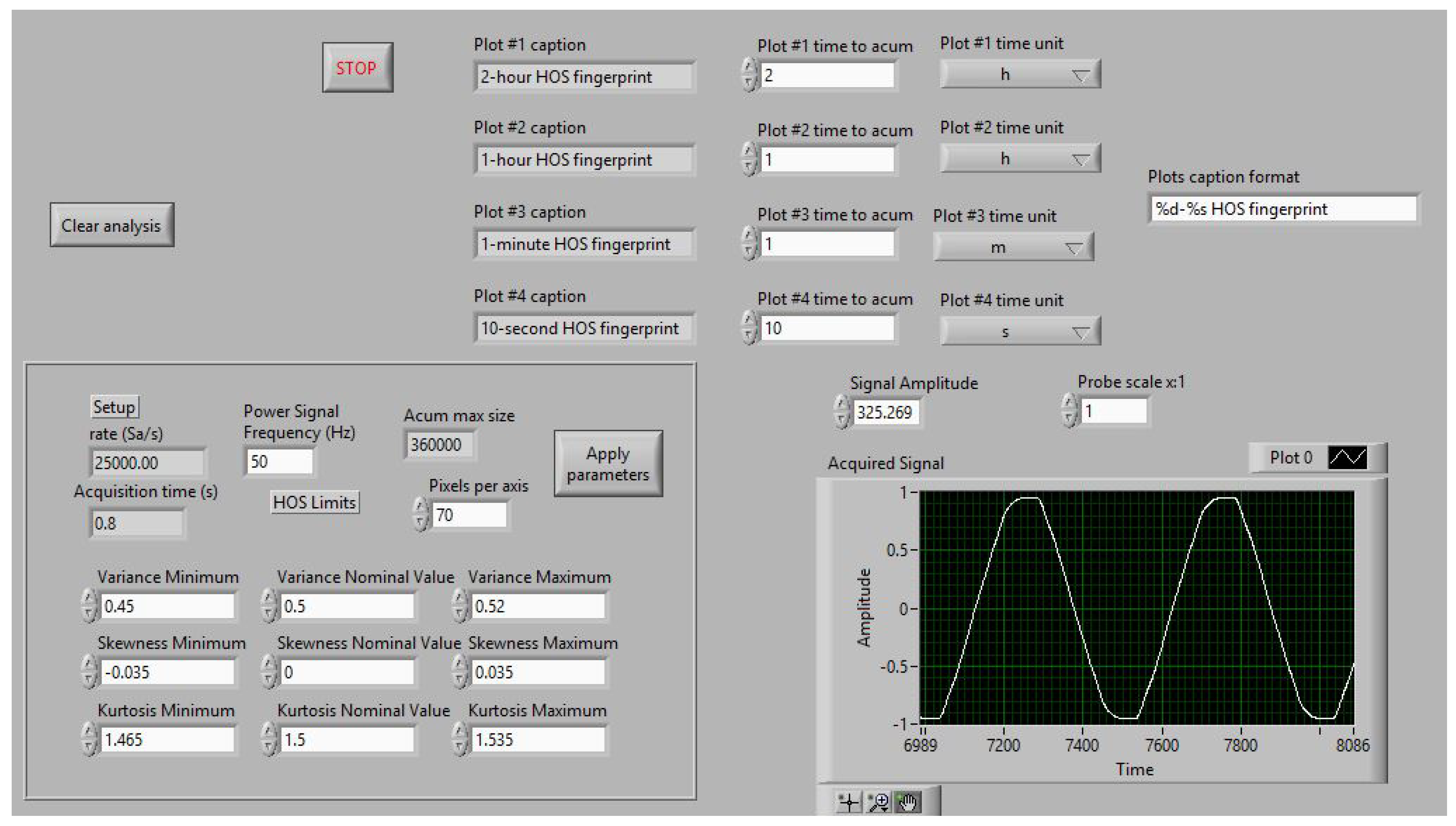
Figure 8.
Flow diagram for the code that implements the trace of the statistics associated to the PQ behaviour.
Figure 8.
Flow diagram for the code that implements the trace of the statistics associated to the PQ behaviour.
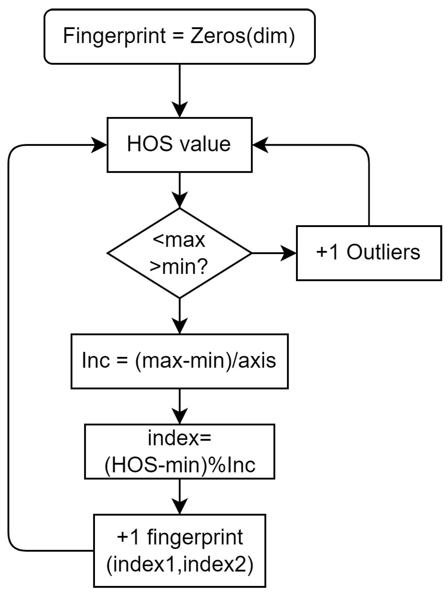
Figure 9.
Histograms for the statistic estimators of the variance, skewness, and kurtosis obtained for averaging times of 1 hour, 1 minute, and 10 seconds, respectively.
Figure 9.
Histograms for the statistic estimators of the variance, skewness, and kurtosis obtained for averaging times of 1 hour, 1 minute, and 10 seconds, respectively.
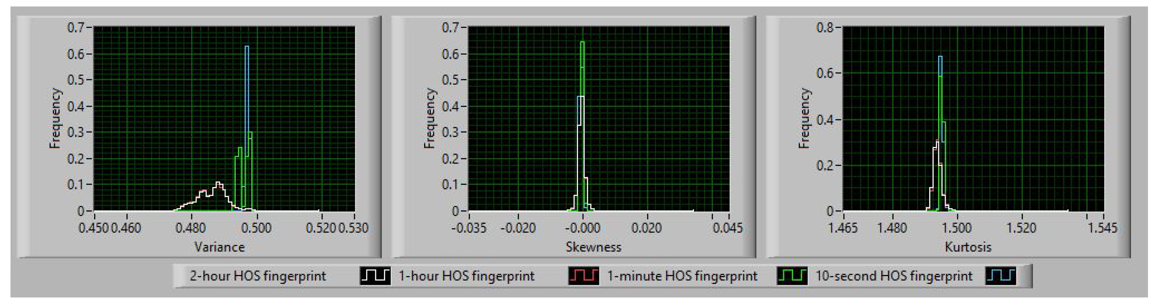
Figure 11.
The programming code that implements the 2D tool path tracing. The associated graphs are depicted in Figure 10.
Figure 11.
The programming code that implements the 2D tool path tracing. The associated graphs are depicted in Figure 10.
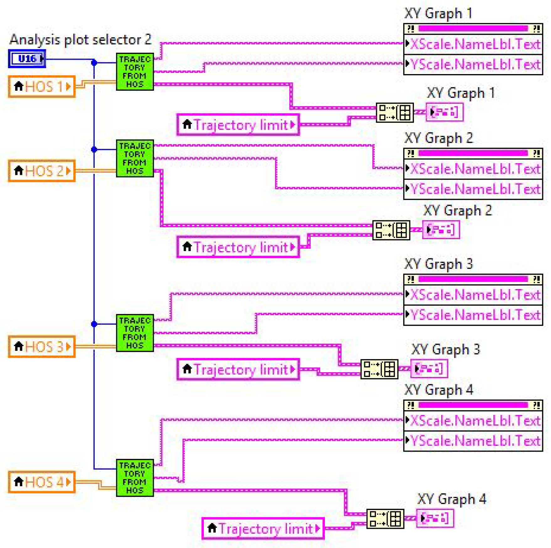
Figure 12.
The programming code that implements the block Trajectories from HOS computing block, included in Figure 11.
Figure 12.
The programming code that implements the block Trajectories from HOS computing block, included in Figure 11.
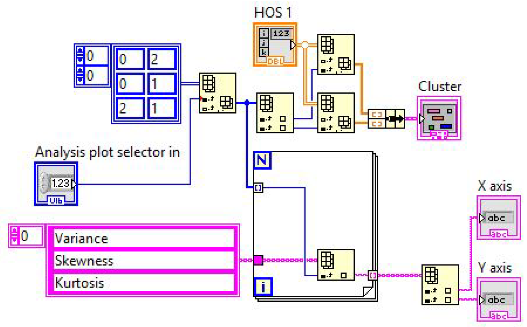

Table 1.
Qualitative performance of indicators: skewness and kurtosis vs. traditional time-domain indices: and CF [2,30].
| Waveform features | Variance and HOS-based indices | Time-domain indices | |||||
|---|---|---|---|---|---|---|---|
| Waveform type | Associated | Variance (var) | Skewness (ske) | Kurtosis (kur) | CF | ||
| distortion | index | ||||||
| Symm-Sinusoidal | Ideal 50 Hz | 0.5 | 0 | 1.5 | 0 | 0.7 | |
| Symm-Sinusoid | Amplitude | Increase-decrease | 0 | 1.5 | Increase | Detect power | |
| (non-phase-angle jump) | (-transient, | (sag-swell) | changes | ||||
| sag, swell, interrup.) | |||||||
| NonSymm-NonSinusoid | Transient, sag, | Increase-decrease | Detect | Detect | Increase | Changes | Detect power |
| (phase-angle jump) | swell, interrup. | (sag-swell) | cycles | phase jump | changes | ||
| of change | (non-sinusoidal) | ||||||
| Symm-NonSinusoid | Harmonic distortion | Increase | 0 | Increase | Increase | Small changes | Detect power |
| -Decrease | changes | ||||||
| NonSymm-NonSinusoid | Other events | Detect changes | Detect changes | Detect changes | Increase | Small changes | Detect power |
| (out of phase-angle jump) | changes | ||||||
Disclaimer/Publisher’s Note: The statements, opinions and data contained in all publications are solely those of the individual author(s) and contributor(s) and not of MDPI and/or the editor(s). MDPI and/or the editor(s) disclaim responsibility for any injury to people or property resulting from any ideas, methods, instructions or products referred to in the content. |
© 2024 by the authors. Licensee MDPI, Basel, Switzerland. This article is an open access article distributed under the terms and conditions of the Creative Commons Attribution (CC BY) license (http://creativecommons.org/licenses/by/4.0/).
Copyright: This open access article is published under a Creative Commons CC BY 4.0 license, which permit the free download, distribution, and reuse, provided that the author and preprint are cited in any reuse.


