
Submitted:
06 December 2024
Posted:
09 December 2024
You are already at the latest version
Abstract
Due to the great demand of pullulan in macromolecular characterization area and its attractive capabilities for chemical engineering towards bio-, farmo-, medical composite materials in DMF solutions we have conducted the classical molecular hydrodynamic study with pullulan standards in dilute DMF solutions. The hydrodynamic characteristics were acquired through viscometry, velocity sedimentation, isothermal diffusion and DLS. The self-consistency check of the obtained values was performed within the concept of hydrodynamic invariant and then the absolute values of molar masses were determined by Svedberg equation. The canonical Kuhn-Mark-Houwink-Sakurada scaling relationships were determined: η, cm^3/g=0.058*M^0.60, s0*10^13, s=0.020*M^0.48 and D_0*10^7,cm^2/s=1300*M^(-0.52) for intrinsic viscosity, sedimentation and diffusion coefficients, correspondingly, within broad molar mass range 7.2≤M_(sD)10^(-3),g/mol≤640. The most sophisticated Gray-Bloomfield-Hearst theory based on implementation of wormlike necklace model resulted in equilibrium rigidity A=(2.4±0.2) nm and transversal polymer chain diameter d=(0.5±0.3) nm. The conformational parameters were also assesed with computer simulations within modern Multi-HYDFIT suite and leaded to close enough data: A_MHF=(3.7±0.3) nm and d_MHF=(2.2±0.2) nm, showing great convergence of classical hydrodynamic theory with computer simulations. The inhere obtained data for pullulan in DMF solutions were also compared with earlier reported results obtained in water revealing nearly identical conformational parameters. Within metrology aspect the acqusiotion of the hydrodynamic characteristics with differenr experimental techniques and their interrelation is discussed in detail.
Keywords:
water soluble polysaccharides
; pullulan
; hydrodynamic methods
; scaling relationships
; Multi-HYDFIT
; conformational parameters
; metrology
1. Introduction
Polysaccharides playing crucial role in living nature are very commonly used in different technological processes, manufacturing and electronics industries, food and pharmaceutical applications. The diversity of polysaccharide applications and their unique properties are determined by all possible variety of their macromolecular architectures, range of equilibrium rigidities of the linear polysaccharide chains, charged/uncharged and/or hydrophilic/hydrophobic interactions within a system, functional end-groups etc. Thus, by studying only polysaccharides the “cornerstone” of polymer science can be established viz. the programing of new material properties based on designing composition at the molecular level.
Pullulan is a linear neutral water-soluble polysaccharide, which consists of α-(1→6) connected maltotriose [1,2,3]. It is mainly obtained from secrets of the fungus Aureobasidium pullulans strains. This was first accomplished by R. Bauer in 1938 [4] and then isolated by B. Bernier in 1958 [5]. Pullulan attracts researchers close attention for a long time by now due to its appealing properties, such as bio-compatibility, bio-reproducibility, being eco-friendly and having endless possibilities for either end-group modifications or synthesizing co-polymers on its basis [6,7,8,9]. Biocompatibility along with the great film-forming ability of pullulan has great potential for the science, medical, food and cosmetic industries [8,9,10,11]. Linear conformation and neutrality makes it a good model example for studying the structure-property relationships in computer simulations and laboratory experiments [12,13]. The possibility of pullulan modification by end-groups of various physicochemical nature opens up wide specter of opportunities for practical applications based on the functions of added groups. The wide range of possible pullulan applications requires for an in-depth study of the conformational behavior and analysis of the relationship between the hydrodynamic and molecular mass parameters of both pullulan itself and its various derivatives in possible solvents [2,14]. The earlier conducted comprehensive studies of pullulan in water accomplished by classical molecular hydrodynamic methods (viscometry, analytical ultracentrifugation, dynamic and static light scattering) revealed the interesting features of this polymer [14,15,16,17,18,19,20]. Further the earlier obtained data were collected and thoroughly analyzed as the whole for determining the conformational parameters of pullulan macromolecules in water in frames of current consistent theoretical models [21]. The determined equilibrium rigidity of a flexible chain polymer and the dependence of scaling indexes of Kuhn-Mark-Houwink-Sacurada equations on molar mass are the factors that are not only fundamental in polymer science, but are also of great practical importance.
One of the popular and beneficial strategies of modern research is designing of the necessary properties of pullulan based systems by its various modifications [6,7,8,22,23]. The final result of modification (the very possibility of modification by certain groups and the degree of substitution) is determined both by the molecular mass characteristics of the polymer and by the environment in which the synthesis is carried out. It has been shown that the use of either DMF or DMF-based binary mixtures improves the parameters of the resulting synthesized macromolecules [10,24].
Thus, the analysis of pullulan hydrodynamic behavior in DMF is the necessary and important task. Nevertheless, there is no systematic comprehensive analysis on pullulan in DMF accomplished up to date which is known to the authors. Taking this into account and considering pullulan standards as well-defined role model with pronouncedly narrow polydispersity the two major goals have been set for the current study. First, the determination of the canonical Kuhn-Mark-Houwink-Sacurada equations for pullulan samples within the large range of molar masses. Second, the metrological aspects have also been tested: the inter correlation of viscometry data obtained with classical Ostwald viscometer and a viscometer working on the Höppler principle, the self-consistency check of the velocity sedimentation data resolved with manual approaches and with that implemented in Sedfit models for acquiring distributions on sedimentation coefficients and molar masses, the convergence test of diffusion coefficients resolved from dynamic light scattering, classical isothermal diffusion and analytical ultracentrifugation data. Finally, the comparison of conformational parameters estimations using both wormlike necklace model within the framework of Gray-Bloomfield-Hearst theory and computer simulations with Multi-HYDFIT suite are considered.
2. Materials and Methods
2.1. Materials
For accomplishing the aims of the current study 11 samples were extensively studied. First 10 standards (the polysaccharide kit, designed for SEC calibration) were purchased from Polymer Laboratories Inc. (Amherst, MA, USA). This kit consists of simple sugars covering oligomer molar mass range (O180, O730) together with relatively narrow polydispersity linear pullulan macromolecules P-1 to P-8. Another pullulan sample (PS) was purchased from Sigma-Aldrich (St. Louis, MO, USA). Unlike pullulan sample standards, this sample exhibited higher polydispersity. The major supplier information on the sample properties (such as batch numbers, weight average molar mass and polydispersity index Ɖ = , where is the number average molar mass) is presented in the Table 1. The shipped samples represented a form of a white to a light yellow powder and they were used as is from the plastically sealed glass vials. The solutions studied in the majority of methods were prepared from the stock solution with reliably determined concentration. The dimethylformamide (DMF) was purchased from Vekton (St. Petersburg, Russia) and it was distilled over calcium hydride under reduced pressure before the experiments. The dynamic viscosity, density and refractive index of purified DMF were determined experimentally at 25 °C and constituted to cP, g/cm3 and , correspondingly.
2.2. Methods
Viscosity measurements (capillary Ostwald and rolling ball Höppler viscometers). The viscous flow of pullulan solutions was studied with two different types of viscometers: first, the classical one capillary Ostwald viscometer (OV) and, second, the commercially available microviscometer Lovis 2000 M (Anton Paar GmbH, Graz, Austria), which implements Höppler principle of rolling ball in a capillary. From here and further the latter viscometer is referred to as rolling ball or Höppler viscometer (HV). The standard dilution procedures were used. The measurements were performed at 25 °C in DMF solutions, which were thermo-stabilized for at least 5 minutes before the measurements. The elution(OV)/rolling ball time(HV) () of DMF and times () of pullulan solutions of various concentration were successively measured during the experiments.
The major differences between the viscometers are as follows: in an OV liquid flows in a vertically positioned capillary with a cross section represented by a circle with a diameter (ranging from 0.227 mm [25]) and up to 1.0 mm commercially available nowadays), on the other hand in a HV a ball rolls in a capillary filled with a liquid while the capillary is positioned at an angle to the horizon pushing a liquid through the gap formed in a shape of “new moon” between the ball and the inner capillary wall (usually, the upper limit in linear gap size mm for low viscous fluids). The comparison of typical values of and makes it clear that a rolling ball viscometer will be much more sensitive for any undesirable impurities (gas bubbles, air dust etc.) capable of entering a liquid, which may lead to distortion of measured time and result in incorrect viscosity values. Thus, the diameter (gap), inner shape of a capillary, the magnitude of its length determine the time of solvent flow, the criteria of flow laminarity and the shear rate of a system under study. The expression for averaged shear rate for capillary OV is presented as follows [26]: , where – the volume of flowed liquid, – the capillary radius and – the elution time. The average shear rate of rolling ball HV is calculated as [27]: , where , – flow behavior index, – the velocity of the ball, – the capillary diameter of HV, – the ball diameter used in HV.
The OV at our disposal has following parameters: = 110 mm,
= 0.34 mm and the elution time of 1 mL of DMF is 50.9 s, which results in ≈ 640 s-1.
In the rolling ball HV the capillary has length = 100.02 mm and diameter = 1.59 mm. The capillary is equipped with a steal ball coated by gold and the ball diameter = 1.5 mm. The angles of the capillary inclination were chosen in the middle of available range and constituted 40 and 50° to the horizon. The lower limit for inclination angles was disregarded due to high sensibility of HV to impurities discussed above and the upper limit may lead to unacceptable turbulence disrupting laminar flow. The time of rolling ball at 40° constituted to (22.83±0.06) s and at 50°: (19.15±0.06) s. Thus, according to Šesták and Ambros [27] the flow behavior index (, where , are the consequent inclination angles and , are the corresponding ball speeds) is estimated as ≈ 1.0, giving function value ≈ 2.4, which in turn resulting in average shear rate ≈ 2100 s-1 at 40° and ≈ 2500 s-1 at 50°, correspondingly. It should be noted, that Lovis 2000 M software installed on HV underestimates the shear rate (490 and 580 s-1, correspondingly at 40 and 50° of inclination) for about 4.5 times in contrast to the calculations above based on the results of [27], which bring much more physically sounded shear rate values especially in comparison with ones obtained on OV, where time of flow and capillary diameter are bigger for the same solvent, but the shear rate value is 640 s-1.
In general, the results of viscosity measurements independently of connotations (either in terms of Huggins [28] or Kraemer equation [29] etc.) the intrinsic viscosity is determined as
where the specific viscosity and relative viscosity .
So, both condition for extrapolation of concentration and shear rate to zero values should be satisfied. However, the viscosity dependence on the shear rate value in the accessible range of the current study for the flexible chain macromolecules with molar mass < 106 g/mol is considered negligible according to [26,30,31]. Accordingly, the difference of viscosity data obtained with OV and HV is associated mostly with difference in viscometers geometry and experimental principles, rather than with difference of shear rate values of OV and HV. However, for rigid chain macromolecules and for samples with molar mass higher than 106 g/mol shear rate extrapolation to zero value must be taken into account for acquiring the true intrinsic viscosity values.
Densitometry. The successive density measurements of pullulan solutions in DMF are necessary for establishing the partial specific volume attributed to the system under study. It allows interpretation of velocity sedimentation data with further determination of absolute molar mass value based on sedimentation-diffusion analysis. The density measurements were performed at = 25 °C, using the density meter DMA 5000 M (Anton Paar GmbH, Graz, Austria). The approach described in Kratky et al. was implemented for data acquisition [32].
Analytical ultracentrifugation (AUC). The velocity sedimentation experiments were accomplished with a ProteomeLab XLI Protein Characterization System analytical ultracentrifuge (Beckman Coulter, Brea, CA). The conventional aluminum double-sector centerpieces with mm optical path length were assembled with sapphire windows into analytical cells and the sectors were filled with 0.42 mL of DMF and 0.41 mL of studied solute, correspondingly. Since a four-hole analytical rotor (An-60Ti) was used it allowed simultaneous studying of three different concentration of a sample at a run. The rotor speeds were 42 000 to 55 000 rpm, depending on the sample. Before the run, the rotor with installed centerpieces was thermostated for approximately 2 hours at 25 °C in the centrifuge vacuumed chamber. Sedimentation profiles were collected during a run at the same temperature using Rayleigh interference optical system equipped with a laser ( = 660 nm).
The result of velocity sedimentation experiment is a set of concentration distributions within an analytical cell recorded with Rayleigh interference system (, where is the interference fringe displacement in relation to the reference sector usually filled with the solvent and is the radius coordinate from the axis of rotation) or optical absorption system (optical density ) at the certain rotor speed and time passed since an experiment start. The concentration distribution within the cell in the first case is attributed to the difference in refractive indexes of solute vs. solvent and in the latter one requires the solute to possess optically active compounds within an available wavelength range of the ultracentrifuge monochromator (190 < , nm < 800).
The sedimentation coefficient value might be calculated manually with its definition ( is the angular rotor velocity) by finding the radial position of sedimentation boundary (considering a sample is presented with a single species) [33]. The procedures for finding have been developed based on differentiations of sedimentation profiles either on radius [33,34,35,36,37] or time [38] resulting in apparent g*(s) coefficient distribution [39,40,41,42,43]. On the other hand there is very powerful Sedfit suite capable of finding sedimentation coefficient distributions [44]. One of the latest Sedfit version (May 2023, v. 16.50) was used. It has lots of built-in models capable to resolve both velocity and equilibrium sedimentation data. It should be mentioned that each model has its advantages and disadvantages in application to resolving velocity sedimentation data of macromolecules (especially in thermodynamically good solvents and/or the solutes with pronounced polydispersity), as the major object of Sedfit preprogramed calculations are biological objects (for example, globular proteins possessing very compact conformation with very distinct size viz. molar mass). The most common ones suited for finding the sedimentation coefficient and molar mass distributions of macromolecules will be discussed and the obtained results will be tested for self-consistency.
The further development of g*(s) into ls-g*(s) model became possible as systematic noise decomposition algorithm was proposed [45]. The appearance of ‘ls’ in the name of the model indicates the least-squares bases of the analysis providing direct fit of sedimentation boundary. This model results in sedimentation coefficient distributions of non-diffusing solutes, so it can be applied to the results of the velocity sedimentation experiments with rather big samples or high rotor speeds where diffusion of the solutes could be omitted otherwise it will show broadening of the obtained distribution due to unaccounted diffusion.
The more advanced model accounting for the diffusion of solutes is continuous c(s) distribution (including continuous c(s) distribution with prior knowledge, viz. c(s) with general scaling law, which is more suitable for resolving sedimentation data of macromolecules) [44]. Both of these models allow to obtain differential distribution on sedimentation coefficient s and a mathematically fitted parameter determining the averaged diffusion coefficient of sedimenting species at measured solution concentration. In case of continuous c(s) model this parameter is frictional ratio , which is the ratio of translational friction of studied sedimenting species to translational friction of equivalent sphere . In the latter model the fitted parameter is entering one of the Kuhn-Mark-Houwink-Sakurada (KMHS) scaling equations relating the sedimentation coefficient and molar mass: . It is worth noticing, that parameters of KMHS equation and can be determined by studying polymer-homologous series of samples of certain polymer also in certain solvent, temperature, molar mass range etc. [46]. So the differential distribution on sedimentation coefficients and parameters characterizing diffusion coefficient are resolved in Sedfit by numerically solving partial differential Lamm equation [47]:
where is the time of applying the centrifugal field at the radius from the axis of rotation with a rotor rotating with an angular speed . First term of the equation describes the diffusion process at the created solution-solvent boundary, which is formed due to the centrifugal field and sedimenting species (second term). Thus, the Sedfit numerically solves Eq. (2) within the given parameters and searches for the least residual values between experimental data and resolved solution, with further implementation of Tikhonov–Phillips regularization procedure [48].
The further advance of velocity sedimentation data treatment was introduced into Sedfit some time ago with implementation of extended Fujita approach [36,49]. This analysis model name is ‘ vs. with scaling law’ (). It allows transformation of differential distribution on sedimentation coefficient into differential distribution on molar mass :
which becomes possible with prior established KMHS equation for the system under study:
or
with . As a result weight average and z-average molar masses may be determined. In previous work [49] authors preliminary suggested estimation of differential distribution on molar mass at lowest possible concentration detectable with AUC optical systems, but in current study the concentration dependence of , , and will be closely considered. The task was accomplished for the majority of the samples with studying at least 3 solution concentrations within about 3-fold of its range. Also the auxiliary parameters (i.e. and ) were determined in this manner.
Diffusion coefficient data. The diffusion coefficients were determined with 3 independent experimental methods. The first estimation of the diffusion coefficient value is possible from velocity sedimentation data processed with continuous distribution model based on sedimentation coefficient and frictional ratio values:
where is the Boltzmann constant and – the absolute temperature on the Kelvin scale. The valued should be treated as estimate since they are calculated with a fitted parameter in the direct experiment on determination of sedimentation coefficient. It was demonstrated earlier, that for various polymer systems the diffusion coefficients evaluated by this approach are indeed reasonable, making the sedimentation velocity analysis completely independent and self-sufficient tool for the molar mass/size determination [50,51,52].At the same time this approach may fall short in its accuracy and suitability for a number of more complex macromolecular systems with more pronounced non-ideal hydrodynamic behavior as well as for rigid chain polymers [50].
Isothermal diffusion (ID). The translational diffusion was studied with Tsvetkov polarizing diffusometer by the classical method of an artificial solution/solvent boundary formation with further observation of diffusion boundary dispersion evolution with Lebedev’s interference scheme [26]. The diffusion boundary is formed in the diffusion cell with a Teflon centerpiece fixed within optical glass plates with an optical path mm along the polarized beam, at average solution concentration of mg/ml. The diffusion data were recorded a digital matrix and further processed with the semiautomatic algorithm [53] for determination of the height and area under the diffusion curve in Gaussian approximation: , where is the dispersion of the diffusion boundary, – the spar twining ( mm) and inverf() – the inverse error function. All experiments were performed at ℃. The translational diffusion coefficients were further calculated by the following equation:
where is the dispersion at the beginning of the experiment characterizing the quality of the boundary formation, and is the time since the start of a diffusion experiment. The evaluated values of the diffusion coefficients were assumed to be the values extrapolated to zero concentration.
Dynamic Light Scattering (DLS). Another independent experiment on the determination of a diffusion coefficient of pullulan samples in DMF was carried out using “PhotoCor Complex” spectrometer (Photocor Instruments Inc., Moscow, Russia). The experimental setup consists of digital correlator (288 channels, 10 ns), a standard goniometer (10°–150°), and a thermostat with temperature stabilization of 0.05 °C. All experiments were carried out at ℃. The single-mode linear polarized laser (wavelength 654 nm) was used as an excitation source; the experiments were carried out within the following range of scattering angles: . Autocorrelation functions of scattered light intensity were processed using the inverse Laplace transform regularization procedure incorporated in DynaLS software (Photocor Instruments Inc., Moscow, Russia), which provides distributions of scattered light intensities by relaxation times . The dependence of (where is the position of a maximum of the distribution) on the scattering vector squared was calculated as , here is a refractive index of a solvent. For all studied samples, this was a straight line passing through the origin, indicating the translation diffusional character of the observed processes () [54]. The concentration dependence of diffusion coefficient was studied for obtaining undisturbed value of diffusion coefficient at the limit of infinite dilution.
Refractometry. The refractive indexes of DMF and refractive index increments were determined with ABBEMAT WR/MW (Anton Paar GmbH, Graz, Austria). Few concentrations of pullulan and oligomer solutions in DMF were studied at nm and ℃. Standard dilution procedures were implemented. It should be noted that refractive index increment may also be assessed through velocity sedimentation and translation diffusion experimental setups equipped with interferometer optical schemes. It was accomplished based on determined jitter displacement at well-defined concentrations: , where nm is the light wavelength, mm is the distance between the interference bands determined by the compensator for Tsvetkov polarizing interferometer and , where μm/pixel is the magnification factor for XLI AUC. The comparison of obtained values with different experimental techniques allows to check the consistency of obtained data.
3. Results and Discussion
3.1. Viscometry
The viscosity experimental data was obtained according to the conditions and using viscometers (OV and HV) described in detail in the experimental section. It was treated both with Huggins [28] and Kraemer [29] equations, where and are Huggins and Kraemer parameters, which are mathematically interrelated as [55,56]. All the data was obtained within the range of relative viscosity: , where they were approximated with linear dependences (Figure S1 and Figure 1). The relative viscosity values obtained with HV at 40 and 50° inclination angles showed practically identical results (Figure 1), so the values were averaged to assess the intrinsic viscosity values. The complete table of determined values of intrinsic viscosities, Huggins and Kraemer parameters with corresponding linear correlation coefficients is presented in Supporting information (Table S1). The determined practically 18-fold range of intrinsic viscosity is in good correlation with assessed molar mass range specified by pullulan sample supplier.The Huggins and Kraemer parameters were averaged for entire range of pullulan samples (oligomers were not included in calculations) and constituted: and , correspondingly (Figure S2). These values satisfy the above interrelation of Huggins and Kraemer parameters within experimental error range. The increase of absolute values of and parameters within studied oligomers molar mass range is most likely caused by imprecision of the slope value evaluation in Huggins and Kraemer plots due to low intrinsic viscosity values and, consequently, insufficient range of measured relative viscosities ( instead of typical for polymer samples ). According to the Table S1 the intrinsic viscosity values determined with Huggins and Kraemer equations were found well correlated and coincided with each other within experimental error. This fact indicates that DMF as a solvent represents thermodynamically good conditions for pullulan macromolecules [57]. So, intrinsic viscosity values and were further averaged to consider the difference of applied experimental techniques, i.e. Ostwald and Höppler viscometers (Table 2). The average discrepancy between intrinsic viscosities determined with Ostwald and Höppler viscometers was determined and turned out to be equal to 3.8 %. The biggest difference of the intrinsic viscosities was found for samples P1, P3 and P4 with up to 5.4 % dissimilarity in absolute values (Figure S3) and on the other hand the obtained data showed the identical values for sample P6. For example, based on earlier published result on intrinsic viscosity values obtained with only capillary viscometers for well-defined samples with close molar mass under the same condition in water solutions the discrepancy of the intrinsic viscosity values varied up to 9.6% (sample P-400 [16] vs. PF806 [15]) or 22% (sample PF308 [15]vs. P-100 [21]). Thus, the coherence of the two data sets obtained with different viscometry experimental techniques may be confirmed. Again, it should be noted that the major difference of these two techniques is mainly associated with extreme sensitivity of HV to any unwanted impurities present in the studied solution due to much lower gap of solution elution in comparison with OV. Consequently, both of the considered inhere viscometers provide reliable results with minor discrepancies associated with regular experimental error. Onward in the current study the intrinsic viscosities (OV and HV) are averaged and used in this manner for further analysis.
3.2. Densitometry
The density of pullulan and oligomer solutions in DMF was measured on the densitometer (Figure S4). Based on the determined slope values , the partial specific volume was determined. It turned out to be equal cm3/g for pullulan samples and cm3/g for the oligomers. The presented slope values were averaged over P2, P7, P8, P9 pullulan samples and separately for both oligomers O180, O730. According to the literature data the partial specific volume was reported earlier for pullulan solutions in water: 0.602 cm3/g [16], (0.61±0.02) cm3/g [20] and 0.65 cm3/g [23]. Therefore, the inhere found values of partial specific volume are in good correlation with previously reported. It is necessary for interpretation of velocity sedimentation data in the following paragraph.
3.3. AUC
The velocity sedimentation data was resolved using two manual techniques ( and ) and four models incorporated in Sedfit: continuous distribution, direct fit of sedimentation boundary based on the least-squares analysis , with ‘general scaling law’ and with extended Fujita approach (Figure 2). All of the models are discussed in detail in experimental section. Also the concentration dependence of the sedimentation coefficients, frictional ratios and pre-exponential coefficients were obtained and undisturbed values (, and ) at zero concentration were determined (Figures S5, S6 and S7). All of the and dependences were linear and approximated by the following expressions and , where is Gralen coefficient and has the same meaning in concertation series of frictional ratio [58]. The sedimentation coefficients resolved in this manner are presented in Table S2. Based on the calculated sedimentation coefficient in infinite dilution limit and Gralen coefficient the Pavlov-Frenkel scaling relationship can be formulated: (Figure S8) [59]. According to the relationship the first estimate of the sedimentation scaling index is made , which will be précised further in the study. Besides, another dimensionless parameter can be calculated for convergence check of the velocity sedimentation and viscometry data (Figure S9). It results in and the upper limit of its value is virtually close to the specific range of to , that is usually found for the flexible macromolecules [60].
The determined sedimentation coefficient range demonstrates 9-fold difference for the studied pullulan samples. One may be immediately convinced that the rotational friction (viscometry) processes in comparison with the translation friction (sedimentation and diffusion) are much more sensible for the size of the studied macromolecular coils, as almost 18-fold difference was determined in intrinsic viscosity values. Also, it is worth noticing, that the sedimentation coefficient S for the lowest molar mass oligomer O180 was found at the bottom range of resolution of the analytical centrifuge. The previously reported findings within the bottom limit of the velocity sedimentation technique were determined for the cyclodextrins [61]. This fact of resolution of such small size species is most likely explained by the narrowest polydispersity of the studied oligomer.
The results obtained by manual processing of sedimentation data (Figure S10) with and techniques are of a control nature. It is mostly due to the fact, that only the main fraction creating the sedimentation boundary may be reliably resolved. Unlike a solution obtained in Sedfit where the distribution on sedimentation coefficients is determined. Yet, the sedimentation coefficients calculated with and technique are in satisfactory agreement with ones obtained with Sedfit distributions (Table S2), as most of the samples have very narrow molar mass distributions (Table 1).
Both continuous and with ‘general scaling law’ models result in practically identical distributions and average sedimentation coefficients (Table S2). This fact is established in identical initial parameters used in the models such as: the range of sedimentation coefficient search, number of test species, confidence level, meniscus and bottom position, solution parameters and boundary conditions for Lamm equation solutions. The only difference of these models is in the resulting fitted parameter: in and in model correspondingly. The model, however, requires the exponential index , which is determined further in the study (Eq. 11). It is also worth noticing that under close inspection of and distributions the negligible low molar mass fractions are detected for almost all studied pullulan samples in the determined sedimentation coefficient range of the studied oligomers ().
The last distributions on sedimentation coefficient resolved with the direct fit of sedimentation boundary based on the least-squares analysis model results in identical results with and models down to pullulan sample P2 (Table S2), where 13% difference in sedimentation coefficient is established. Further comparison of sedimentation coefficients for sample P1 results in 30% difference. It means, that the model applicability limit is reached at about 2 S. In the determined size range the diffusion process can no longer be unaccounted and results in not only in distribution broadening, but also affects the value of the sedimentation coefficient. The similar observations were made earlier for other macromolecular systems [58,62].
Finally, the velocity sedimentation data was treated with implementation of model with extended Fujita approach (Table S2). It is also as model requires the knowledge of exponential index for the system under study. According to the resolved data (Table S2) for successful determination of true weight average , z-average molar masses and corresponding distribution the following criteria can be formulated. First, the calculated sedimentation coefficient of the corresponding studied solution concentration must be in immediate vicinity of the determined sedimentation coefficient in the limit of infinite dilution. Second, the value fitted with both and models for the solution concentration under consideration is in the experimental error range determined independently in KMHS equations. Third, the velocity sedimentation data should be collected at the lowest concentration, which allows reliable data resolution within the frame of and Sedfit models. In that case the satisfactory correlation of , and the absolute molar mass (determined further in the study, Table 3) obtained with sedimentation-diffusion analysis can be established. Indeed, for the pullulan samples from P1 to P7 the comparison of with the absolute molar mass values obtained by sedimentation diffusion analysis is within the 5% difference, which can be considered as experimental error range. On the other hand, the difference of with for pullulan sample P8 is almost about 70%. This is definitely explained by strongly expressed concentration dependence of the hydrodynamic parameters, viz. the sedimentation coefficient and more important the value (Figures S5 and S7). Although both and value of P8 sample are assessed in condition of very diluted solution, where dilution parameter (Figure S7), the value fitted with and independently in models was found to be equal to , which is quite different with the . Due to this difference and according to the equation the weight average molar mass resolved with model gives strongly overestimated value. It means, that for high molar mass samples with strongly expressed concentration dependence the velocity sedimentation experiments must be performed at . This may be achieved by performing the experiments at extremely low concentrations with one of the following techniques: the engaging of absorbance optical system for the certain samples capable to absorb at the available range of XLI monochromator, modifying the system under study with fluorescent labels and using fluorescent detector [63] or using commercially available 20 mm centerpieces for AUC cells [64]. None of the above listed is in our possession at the moment, so the resolution of high molar mass pullulan samples with model is a matter of further studies. Nevertheless, the earlier formulated criteria and current state of our experimental apparatus allowed trustworthy well-correlated solution with model for a flexible chain macromolecule (pullulan) in the thermodynamically good solvent for up to 420000 g/mol in molar mass. For example, Figure S11 demonstrates the comparison of pullulan sample P5 with PS, which have close molar mass values, but polydispersity of the samples is quite different. It would seem, that the difference of the determined 1.05 and 1.31 in polydispersity index is not high in value, but it shows crucial change in both distribution on sedimentation coefficient and molar mass, correspondingly. It should be noted, that polydispersity index for PS was not provided by supplier and it was determined in this study. It also might be a little underestimated, as it is found with ratio of third average moment () of molar mass to the second one () and due to the fact that the distribution was not resolved properly in oligomer range, so these low molar mass species are excluded from the analysis. The slight underestimation of the polydispersity index is confirmed for pullulan sample P5. The supplier data for the sample is 1.12 in comparison with 1.05 determined inhere with model. The similar trend is established for other pullulan samples (Table S3).
Thus, for the first time to the best of the authors’ knowledge the concentration effect on molar mass distribution is obtained, studied and the criteria for reasonable resolution of velocity sedimentation data with the Sedfit model are formulated.
3.4. Diffusion Experiments and the Concept of Hydrodynamic Invariant
The diffusion coefficients were assessed independently with three different experimental techniques: isothermal diffusion () studied with polarizing Tsvetkov diffusometer (Figure 3), the diffusion coefficients obtained by continuous distribution model implemented in Sedfit calculated with sedimentation coefficients and frictional ratio values (Eq. 6) (Figures S5 and S6) at infinite dilution limit () and – dynamic light scattering (Figure S12). This is another raised question addressed towards methodology area in regard to explore the convergence of results and exploring limits of engaged experimental approaches. The obtained data are presented in Table S4. It can be seen that the diffusion coefficients obtained by the three independent experiments for every sample are in satisfactory agreement with each other and for the most samples are found practically within experimental error range.
At this point of study, the intrinsic viscosities and velocity sedimentation coefficients of pullulan samples in DMF are reliably determined, so the concept of hydrodynamic invariant [65] may be implemented to ensure, that the determined diffusion coefficients are well correlated with earlier discussed data. Besides, it is very convenient moment for hydrodynamic characteristic self-consistency check, as diffusion coefficient influence hydrodynamic invariant in higher power, than intrinsic viscosity and sedimentation coefficient:
where is universal gas constant, and are characteristic diffusion and sedimentation coefficients, correspondingly. The hydrodynamic invariant values were calculated for all obtained diffusion coefficients. It was found, that practically all of values are physically sounded and belong to the range of the theoretical value known for hard spheres and to cm2g/(s2K mol1/3) for Gaussian chains in the absence of volume effects and in the limit of preaveraging of the hydrodynamic Oseen’s tensor [65], except for two diffusion coefficients evaluated for oligomers with DLS. Indeed, the oligomer sizes are over the resolution limit of the experimental set up. Thus, all other diffusion coefficients were averaged and used further in the study in this manner. This allows to combine all obtained hydrodynamic characteristics in general table (Table 3). The Table 3 contains the absolute molar masses, which were calculated with Svedberg equation:
the hydrodynamic invariant values determined with Eq. (9) and the sedimentation parameter that has the same properties as [60]:
where is the Avogadro constant. ). For the studied pullulan sample series, the following average values of hydrodynamic invariants were obtained: cm2g/(s2K mol1/3) and mol-1/3. It well correlates with earlier published data [21,58,60,66,67,68,69]. After making sure that the hydrodynamic characteristics are consistent, one can proceed to further interpretation of the obtained matrix of experimental hydrodynamic values and molar masses of polymer homologues.
3.5. Refractive Index Increment
Since the major experimental results have been obtained at this point of study, it is possible to summarize and compare data on refractive index increment obtained with optical interferometer detection schemes (Rayleigh’s in AUC [70] and Lebedev’s in isothermal diffusion [26]) and refractometer (Figure S13). The data are presented in Table S5. It can be seen, that obtained values are in satisfactory agreement within each technique, so the average values can be discussed: (0.08±0.01), (0.096±0.002) and (0.101±0.001) cm3/g, which are related to isothermal diffusion, AUC and refractometer, correspondingly. There was not observed noticeable difference in refractive index increment of pullulan samples and its oligomers. It should be noticed, that and are in average lower than . This might be explained by presence of negligible presence of oligomeric fraction also resolved with AUC distributions. The slight difference between and most probably obtained by both the difference in light wavelength value and construction features of interferometers build in experimental set ups.
3.6. Hydrodynamic Scaling Relationships
The interrelation of hydrodynamic characteristics of macromolecules with each other and with molar mass allows to obtain two types of scaling relationships. One is well known type of scaling relationships between hydrodynamic characteristics and molar masses or Kuhn-Mark-Houwink-Sakurada (KMHS) equations (Figure 4). Other type is interrelationships among hydrodynamic characteristics. The whole set of relationships, may be parameterized and given as follows:
where is one of the hydrodynamic characteristics , , , , and is another corresponding hydrodynamic characteristic or molar mass. It should be noted, that either type of scaling relationships is describing polymer homologous series at certain conditions (solvent, temperature, the ion strength of a solution etc.) within determined molar mass range. Cross plots (hydrodynamic characteristics vs. other hydrodynamic characteristics) make it possible to verify how much the pair of initial characteristics obtained by various hydrodynamic methods correlate with each other (Figure S14). The case of a noticeable deviation of some pair of them indicates the need to verify the experimental results. The plots of such cross-correlations are shown in Figure S14. Table S6 summarizes the parameters of the entire set of derived scaling relationships, which demonstrate satisfactory cross-correlations between various experimental characteristics. Table 4 and figure KMHS contain data on canonical KMHS scaling relationships. Taking into account the well-known interrelation of scaling indexes ( and ) the final view of KMHS relationships reads as
for pullulan macromolecules within the molar mass range in DMF solutions at 25 °C for intrinsic viscosity, velocity sedimentation and diffusion coefficients, correspondingly.
Considering the intrinsic viscosity values (most sensible characteristic to size of the species) of oligomer molar mass range, the tendency towards decreasing of may be noticed, which in turn means the lower effect of oligomer size on the hydrodynamic parameters. The scaling indexes are not calculated within the oligomer range due to the scarce of available data points. The situation with the number of available data points was radically different in the study of pullulan homologous series in H2O [15,16,17,18,20], where besides the determined within the study hydrodynamic characteristics, those were also summarized with previously reported data [21] resulting in overall analysis of independently acquired hydrodynamic characteristics on 81 independent samples within the record molar mass range . This in turn allowed the resolution of two reliably determined sets of scaling indexes within following molar mass ranges. First set of scaling indexes was resolved for the molar mass range and resulted in , , where is a scaling indexes relating translation friction coefficients ( or equivalently ) vs. molar mass in log-log scale. The second one () leaded to , . The comparison of scaling indexes obtained in this study with ones, obtained earlier for pullulan study in water solutions results in following conclusions: the similar decrease in value was observed for oligomer range in water solutions, which proves the earlier made point on the lower effect of the oligomer size on the hydrodynamic parameters. While the larger value of in the second molar mass range may indicate higher demonstration of excluded volume effects in water solutions, the structural parameter responsible for draining affects viz. the diameter of a pullulan chain is the same in both environments (DMF and H2O).
Figure 4.
The double logarithmic plot of KMHS scaling relationships for intrinsic viscosity (1), sedimentation coefficients (2) and diffusion coefficients (3) obtained for pullulan samples in DMF solutions at 25 °C. The red data points refer to oligomer hydrodynamic characteristics and were not included into analysis.
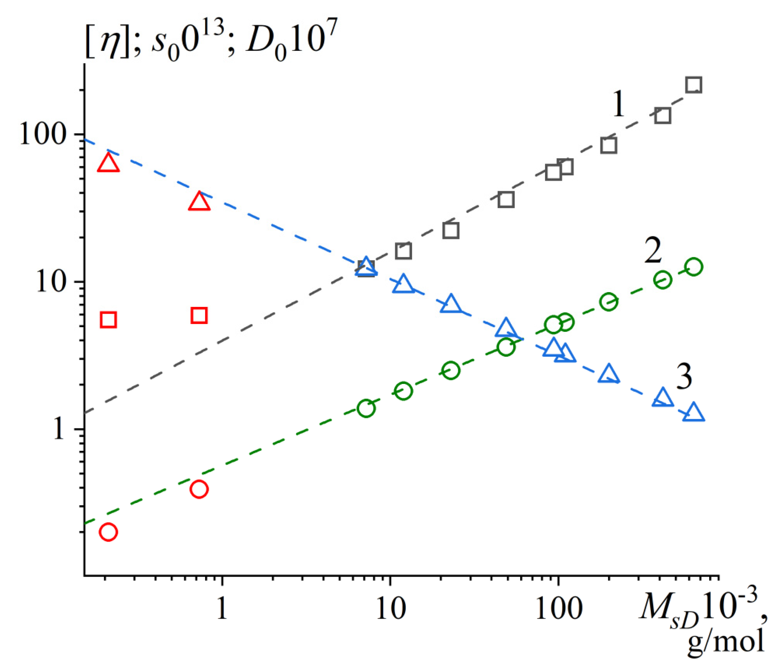

Table 4.
Parameters of scaling KMHS relationships for pullulan samples in DMF at 25 °C.
| 1 | |||
| 0.62±0.02 | 0.044±0.009 | 0.9970 | |
| 0.49±0.01 | 0.017±0.001 | 0.9999 | |
| -0.51±0.01 | 1110±50 | -0.9998 |
1 The linear correlation coefficients of corresponding double logarithmic dependences (Figure 4).
3.7. Determination of Conformational Parameters
The equilibrium rigidity and transversal diameter of a pullulan chain will be determined with the most sophisticated Gray-Bloomfield-Hearst theory [71], which is taking into account both excluded volume effects and draining effects. Then the conformational characteristics will also be assessed through the Monte Carlo simulations using a worm-like general model when processing the entire array of hydrodynamic data, which was relatively recently [72,73,74]. In this method, a common solution is sought that best fits the experimental data obtained by several independent methods, in our case, data on the translational friction of macromolecules in solutions (velocity sedimentation and translational diffusion), as well as the results of their viscous friction in dilute solutions (intrinsic viscosity).
The Gray-Bloomfield-Hearst theory describes the dependence of the sedimentation coefficient of a wormlike necklace and in the region ( is the contour length of a chain) the model expression reads as follows [71]:
where =5.11 is the translational friction Flory coefficient, – the molar mass per unit chain length, – the parameter characterizing thermodynamic quality of the solvent and is the parametrized function . Besides using the substitute , where is rotational friction Flory coefficient, in Eq. (12) [75] both translational (velocity sedimentation and diffusion) and rotational (viscometry) friction data can be processed. It allows the determination of equilibrium rigidity , and effective transversal diameter , of a polymer chain depending on the extrapolated data type (indexes – rotational friction data and – translational one). To acquire the conformation parameters the molar mass per unit chain length must be determined. Here is the molar mass of a monomer unit of pullulan and is the projection of a monomer unit to the direction of fully extended polymer chain. is known with the polymer unit structure and equals to 162 g/mol and cm [16] per glucopyranose ring, resulting in g/(mol cm).
It should be noted that value may be assessed based on the hydrodynamic experimental data using a weakly bended cylinder model. The model is relevant for the following range of the relative polymer chain contour length: and reads as [76]:
Due to the fact that pullulan is a flexible chain polymer to satisfy the condition on the relative polymer chain contour length only two data points acquired in this study (O180 and O738) may be considered for the Eq. (13) model plot. Despite of the fact the experimental value is calculated with almost 100% experimental error it results in close to the theoretical calculation g/(mol cm) on the upper error limit g/(mol cm) (Figure S15).
Also, besides the the parameter characterizing thermodynamic quality of the solvent must be determined. This was accomplished by implementing the following expressions , which resulted in the average value . Thus, according to Eq. (12) and corresponding plots of the in here obtained experimental data at the Figure S16 the following values of equilibrium rigidity nm, nm and transversal diameter nm, nm are obtained, which result in average values nm and nm characterising the pullulan macromolecules in DMF solution extensively studied in current project. On the other hand the average values for conformational parameters characterizing pullulan in water medium read as follows: nm and nm. Thereby due to practically identical results the consistency of hydrodynamic data obtained in water and DMF environment is established, as well both the excluded volume effects and draining effects within the frames of Gray-Bloomfield-Hearst theory may be considered greatly handled. The last column of Table 3 gives the number of statistical segments in the pullulan chains, which demonstrates its range for the studied pullulan samples.
3.8. Multi-HYDFIT Suite
Hydrodynamic coefficients, solution properties and ultimately conformational parameters of the macromolecules can be calculated using Multi-HYDFIT [72,73,74]. Engaging Monte Carlo simulation the program Multi-HYDFIT allows processing of hydrodynamic data for practically any sort of macromolecules, covering the full range of the worm-like model, from short cyllinders to very long, fully flexible chains. The main block of hydrodynamic data (, , , and ) is entered into the program, as well as the parameters characterizing solution , , and , which are necessary for the transition to the characteristic values and .
The persistence length (which is related to equilibrium rigidity as ), transversal diameter () of a chain and mass per unit length () can be evaluated using Multi-HYDFIT program; this program performs a minimization procedure aimed at finding the best values of , and satisfying the conditions of the chosen theoretical model. The Multi-HYDFIT program then “floats” the variable parameters in order to find a minimum of the target function , which is calculated through equivalent radii [73]:
where is the equivalent radius (defined as a radius of an equivalent sphere having the same value as the determined characteristic (translation diffusion , velocity sedimentation coefficients and intrinsic viscosity )), is the overall number of samples, is the weights for the various hydrodynamic properties, the indexes and indicate calculated and experimental values, correspondingly. The error function is a dimensionless estimate of the agreement between the experimentally measured characteristic and the theoretical values of , and calculated for the selected hydrodynamic characteristic and for a particular molar mass. Thus, can be regarded as a typical difference between the calculated and experimental values for the whole set of properties of the series of samples. Multi-HYDFIT allows to fit any of the parameters (, and ) or fix the value of either one of them to calculate the other two.
The final results of Multi-HYDFIT program are presented as the color gradient maps of conformation-structural parameters like a topographic map (Figure 5). The color gradient is set by the value of the error function, consequently the solution is presented by the region with the lowest value of . This is illustrated in Figure 5, which demonstrates the result of Multi-HYDFIT handling hydrodynamic data obtained for pullulan samples in DMF and water dilute solutions. The Multi-HYDFIT simulations were launched for the obtained hydrodynamic parameters obtained inhere () and independently with summarized pullulan data () in water solutions [21].
Table 4.
The structural parameters of pullulan chains resolved independently from hydrodynamic characteristics obtained in DMF and H2O environment with Multi-HYDFIT program: persistence length (), transversal diameter of a chain (), molar mass per unit length of a chain () and target delta function ().
| Solvent | Variables | Fixed values |
, nm |
, nm |
, g/(mol cm) |
Δ, % |
| DMF | 1.9 ± 0.1 | 2.0 ± 0.2 | 3.6 ± 1.2 | 12.7 | ||
| DMF | 2.0 ± 0.1 | 2.2 ± 0.2 | 3.38 | 7.6 | ||
| H2O | 1.8 ± 0.1 | 1.8 ± 0.1 | 4.1 ± 0.3 | 14.8 | ||
| H2O | 1.7 ± 0.1 | 1.8 ± 0.1 | 3.38 | 15.0 |
The main results of Multi-HYDFIT solutions for two separate sets of hydrodynamic data on pullulan in DMF and H2O at 25 °C are presented in Figure 5 and Table 4. It can be seen, that independently of the computer data simulation the program returns very consistent data on persistent length and the transversal diameter of a pullulan chain. The average values in notations of equilibrium rigidity and transversal diameter are nm and nm, correspondingly, for the Multi-HYDFIT runs with the fixed theoretically calculated molar mass per unit length of a chain value g/(mol cm). Again, as it was noticed earlier [77] the value search by the Multi-HYDFIT results in closer to theoretical calculation value, as the oligomer molar mass range is filled with hydrdyanmic data within the range of relative contour length . The equilibrium rigidity resolved with Multi-HYDFIT is close to averaged one determined with Gray-Bloomfield-Hearst theory allowing to refer to pullulan as flexible chain polymer. The data resolved with the two independent approaches may be considered in satisfactory agreement. The transversal diameter of a polymer chain is often calculated with large error due to the difficulty of its determination. Based on Multi-HYDFIT solution and calculations of Gray-Bloomfield-Hearst theory its range of possible values is determined as follows: . Additionally, its value may be assessed through the following equation, which interrelates the partial specific volume to under purely geometrical assumption by representing the molar mass per unit chain length as a cylinder with uniformly distributed material [78]:
The Eq. (15) leads to the following transversal diameter value nm. It indeed belongs to previously determined range and its value is closer to calculations with Gray-Bloomfield-Hearst theory.
4. Conclusions
According to the main raised goals in the beginning of the study we have completed the self-consistent study of pullulan standards in DMF solutions within record 3 order of magnitude range of molar mases with the set of molecular hydrodynamic methods. Then the self-consistency check was performed within the concept of the hydrodynamic invariant and the absolute molar masses have been determined. It allowed the determination of the canonical Kuhn-Mark-Houwink-Sakurada relationships for pullulan samples in DMF solutions at 25 °C. The comparison of viscometry data on the studying the same solution with classical Ostwald viscometer and a viscometer working on the Höppler principle revealed up to ~5% difference in intrinsic viscosities values, which can be considered as experimental error and thereby obtained data are treated as indistinguishable from experimental point of view. The major determining factor for the observed difference in viscometry data is the greater sensitivity the Höppler viscometer to any solution impurities in comparison with Ostwald one. The velocity sedimentation data obtained with manual approach and with Sedfit models resulted in practically identical sedimentation coefficient values. The overestimation of sedimentation coefficients with ls-g*(s) model was observed for low molecular samples ( S). For the first time the concentration dependence of distribution obtained with fgsl(M) was considered and necessary criteria was formulated for determination of true molar mass distributions and the averaged molar mass values. The diffusion coefficient obtained with three independent experimental approaches resulted in close values, which convergence was established within the concept of hydrodynamic invariant. The experimental limits of DLS technique were determined for pullulan oligomers of low sizes. Finally, the satisfactory correlation of the determined conformational parameters for independent studies on pullulan in dilute DMF (obtained in here) and water (reported earlier) solution, resolved with Gray-Bloomfield-Hearst theory and Multi-HYDFIT suite was established. The obtained range of equilibrium rigidity determines the pullulan in DMF as flexible chain polymer in thermodynamically good solvent. The importance of samples within the oligomer molar mass range (L/A < 2 region) for correct resolution of parameter with Multi-HYDFIT suite has been demonstrated.
Supplementary Materials
The following supporting information can be downloaded at the website of this paper posted on Preprints.org. Figure S1-S3 and Table S1 present viscometry data and its interpretation; Figure S4 – densitometry; Figure S5-S11 and Table S2 – velocity sedimentation data analysis; Figure S12 and Table S4 – DLS and diffusion data; Figure S13 and Table S5 – refractive index increment data; Figure S14-S16 and Table S6 – KMHS scaling relationships and theoretical models.
Author Contributions
Conceptualization, A.S.G. and G.M.P.; methodology, A.S.G. and G.M.P.; validation, A.S.G., O.O.V., A.A.L., A.I.K., M.M.E. and G.M.P.; formal analysis, A.S.G., O.O.V., A.A.L., A.I.K., M.M.E. and G.M.P.; investigation, A.S.G., O.O.V., A.A.L., A.I.K., M.M.E.; data curation, A.S.G., O.O.V., A.A.L., A.I.K., M.M.E. and G.M.P.; writing—original draft preparation, A.S.G. and G.M.P.; writing—review and editing, A.S.G., O.O.V., A.A.L., A.I.K., M.M.E. and G.M.P.; visualization, A.S.G., O.O.V., A.A.L., A.I.K., M.M.E.; supervision, A.S.G. and G.M.P.; project administration, A.S.G. and G.M.P. All authors have read and agreed to the published version of the manuscript.
Funding
This research was financially supported by the Russian Science Foundation (project no. 22-13-00187, https://rscf.ru/project/22-13-00187/).
Institutional Review Board Statement
Not applicable.
Acknowledgments
The authors are grateful to the Research Park of St. Petersburg State University, namely the Centre for Diagnostics of Functional Materials for Medicine, Pharmacology and Nanoelectronics.
Conflicts of Interest
The authors declare no conflicts of interest.
References
- Leathers, T.D. Biotechnological production and applications of pullulan. Appl. Microbiol. Biotechnol. 2003, 62, 468–473. [Google Scholar] [CrossRef] [PubMed]
- Singh, R.S.; Kaur, N.; Singh, D.; Bajaj, B.K.; Kennedy, J.F. Downstream processing and structural confirmation of pullulan - A comprehensive review. Int. J. Biol. Macromol. 2022, 208, 553–564. [Google Scholar] [CrossRef] [PubMed]
- de Souza, C.K.; Ghosh, T.; Lukhmana, N.; Tahiliani, S.; Priyadarshi, R.; Hoffmann, T.G.; Purohit, S.D.; Han, S.S. Pullulan as a sustainable biopolymer for versatile applications: A review. Materials Today Communications 2023, 36, 106477. [Google Scholar] [CrossRef]
- Bauer, R. Physiology of Dematium Pullulans de Bary. Zentralbl. Bacteriol. Parasitenkd. Infektionskr. Hyg. Abt. 2 1938, 98, 133–167. [Google Scholar]
- Bernier, B. THE PRODUCTION OF POLYSACCHARIDES BY FUNGI ACTIVE IN THE DECOMPOSITION OF WOOD AND FOREST LITTER. Can. J. Microbiol. 1958, 4, 195–204. [Google Scholar] [CrossRef]
- Liu, Z.; Jiao, Y.; Wang, Y.; Zhou, C.; Zhang, Z. Polysaccharides-based nanoparticles as drug delivery systems. Advanced Drug Delivery Reviews 2008, 60, 1650–1662. [Google Scholar] [CrossRef]
- Agrawal, S.; Budhwani, D.; Gurjar, P.; Telange, D.; Lambole, V. Pullulan based derivatives: synthesis, enhanced physicochemical properties, and applications. Drug Delivery 2022, 29, 3328–3339. [Google Scholar] [CrossRef]
- Danjo, T.; Enomoto, Y.; Shimada, H.; Nobukawa, S.; Yamaguchi, M.; Iwata, T. Zero birefringence films of pullulan ester derivatives. Scientific Reports 2017, 7, 46342. [Google Scholar] [CrossRef]
- Singh, R.S.; Kaur, N.; Kennedy, J.F. Pullulan and pullulan derivatives as promising biomolecules for drug and gene targeting. Carbohydr. Polym. 2015, 123, 190–207. [Google Scholar] [CrossRef]
- Guerrini, L.M.; Oliveira, M.P.; Stapait, C.C.; Maric, M.; Santos, A.M.; Demarquette, N.R. Evaluation of different solvents and solubility parameters on the morphology and diameter of electrospun pullulan nanofibers for curcumin entrapment. Carbohydr. Polym. 2021, 251, 117127. [Google Scholar] [CrossRef]
- Ajalloueian, F.; Asgari, S.; Guerra, P.R.; Chamorro, C.I.; Ilchenco, O.; Piqueras, S.; Fossum, M.; Boisen, A. Amoxicillin-loaded multilayer pullulan-based nanofibers maintain long-term antibacterial properties with tunable release profile for topical skin delivery applications. Int. J. Biol. Macromol. 2022, 215, 413–423. [Google Scholar] [CrossRef]
- Liu, J.H.Y.; Brameld, K.A.; Brant, D.A.; Goddard, W.A. Conformational analysis of aqueous pullulan oligomers: an effective computational approach. Polymer 2002, 43, 509–516. [Google Scholar] [CrossRef]
- Perez-Moral, N.; Plankeele, J.-M.; Domoney, C.; Warren, F. Ultra-high performance liquid chromatography-size exclusion chromatography (UPLC-SEC) as an efficient tool for the rapid and highly informative characterisation of biopolymers. Carbohydr. Polym. 2018, 196. [Google Scholar] [CrossRef]
- Nishinari, K.; Fang, Y. Molar mass effect in food and health. Food Hydrocolloids 2021, 112, 106110. [Google Scholar] [CrossRef]
- Kato, T.; Okamoto, T.; Tokuya, T.; Takahashi, A. Solution properties and chain flexibility of pullulan in aqueous solution. Biopolymers 1982, 21, 1623–1633. [Google Scholar] [CrossRef]
- Kawahara, K.; Ohta, K.; Miyamoto, H.; Nakamura, S. Preparation and solution properties of pullulan fractions as standard samples for water-soluble polymers. Carbohydr. Polym. 1984, 4, 335–356. [Google Scholar] [CrossRef]
- Kato, T.; Katsuki, T.; Takahashi, A. Static and dynamic solution properties of pullulan in a dilute solution. Macromolecules 1984, 17, 1726–1730. [Google Scholar] [CrossRef]
- Buliga, G.S.; Brant, D.A. Temperature and molecular weight dependence of the unperturbed dimensions of aqueous pullulan. Int. J. Biol. Macromol. 1987, 9, 71–76. [Google Scholar] [CrossRef]
- Pavlov, G.M.; Yevlampieva, N.P.; Korneeva, E.V. Flow birefringence of pullulan molecules in solutions. Polymer 1998, 39, 235–239. [Google Scholar] [CrossRef]
- Nishinari, K.; Kohyama, K.; Williams, P.A.; Phillips, G.O.; Burchard, W.; Ogino, K. Solution properties of pullulan. Macromolecules 1991, 24, 5590–5593. [Google Scholar] [CrossRef]
- Pavlov, G.M.; Korneeva, E.V.; Yevlampieva, N.P. Hydrodynamic characteristics and equilibrium rigidity of pullulan molecules. Int. J. Biol. Macromol. 1994, 16, 318–323. [Google Scholar] [CrossRef] [PubMed]
- Tiwari, S.; Patil, R.; Dubey, S.K.; Bahadur, P. Derivatization approaches and applications of pullulan. Adv. Colloid Interface Sci. 2019, 269, 296–308. [Google Scholar] [CrossRef] [PubMed]
- Zorin, I.M.; Fetin, P.A.; Mikusheva, N.G.; Lezov, A.A.; Perevyazko, I.; Gubarev, A.S.; Podsevalnikova, A.N.; Polushin, S.G.; Tsvetkov, N.V. Pullulan-Graft-Polyoxazoline: Approaches from Chemistry and Physics. Molecules 2024, 29. [Google Scholar] [CrossRef]
- Pereira, J.M. Synthesis of New Pullulan Derivatives for Drug Delivery. PhD Dissertation of the Virginia Polytechnic Institute and State University, 2013.
- Ostwald, W.; Malss, H. Über Viskositätsanomalien sich entmischender Systeme, I. Über Strukturviskosität kritischer Flüssigkeitsgemische. Kolloid-Zeitschrift 1933, 63, 61–77. [Google Scholar] [CrossRef]
- Tsvetkov, V.N.; Eskin, V.E.; Frenkel, S.Y. Structure of Macromolecules in Solution; The National Lending Library for Science and Technology: Boston, 1971; p. 762. [Google Scholar]
- Šesták, J.; Ambros, F. On the use of the rolling-ball viscometer for the measurement of rheological parameters of power law fluids. Rheol. Acta 1973, 12, 70–76. [Google Scholar] [CrossRef]
- Huggins, M.L. The viscosity of dilute solutions of long-chain molecules. I. J. Phys. Chem. 1938, 42, 911–920. [Google Scholar] [CrossRef]
- Kraemer, E.O. Molecular Weights of Celluloses and Cellulose Derivates. Ind. Eng. Chem. 1938, 30, 1200–1203. [Google Scholar] [CrossRef]
- Zimm, B.H. Dynamics of Polymer Molecules in Dilute Solution: Viscoelasticity, Flow Birefringence and Dielectric Loss. The Journal of Chemical Physics 1956, 24, 269–278. [Google Scholar] [CrossRef]
- Kuhn, W.; Kuhn, H. Bedeutung beschränkt freier Drehbarkeit für die Viskosität und Strömungsdoppelbrechung von Fadenmolekellösungen I. Helv. Chim. Acta 1945, 28, 1533–1579. [Google Scholar] [CrossRef]
- Kratky, O.; Leopold, H.; Stabinger, H. The determination of the partial specific volume of proteins by the mechanical oscillator technique. Methods Enzymol. 1973, 27, 98–110. [Google Scholar] [CrossRef]
- Svedberg, T.; Pedersen, K.O.; Bauer, J.H. The Ultracentrifuge; Oxford University Press: New York, 1940; p. 478. [Google Scholar]
- Baldwin, R.L.; Williams, J.W. Boundary spreading in sedimentation velocity experiments. J. Am. Chem. Soc. 1950, 72, 4325–4325. [Google Scholar] [CrossRef]
- Bridgman, W.B. Some Physical Chemical Characteristics of Glycogen. J. Am. Chem. Soc. 1942, 64, 2349–2356. [Google Scholar] [CrossRef]
- Fujita, H. Mathematical Theory of Sedimentation Analysis. 1962.
- Signer, R.; Gross, H. Ultrazentrifugale Polydispersitätsbestimmungen an hochpolymeren Stoffen. 95. Mitteilung über hochpolymere Verbindungen. Helv. Chim. Acta 1934, 17, 726–735. [Google Scholar] [CrossRef]
- Stafford, W.F. Boundary analysis in sedimentation transport experiments: A procedure for obtaining sedimentation coefficient distributions using the time derivative of the concentration profile. Anal. Biochem. 1992, 203, 295–301. [Google Scholar] [CrossRef]
- Frigon, R.P.; Timasheff, S.N. Magnesium-induced self-association of calf brain tubulin. I. Stoichiometry. Biochemistry 1975, 14, 4559–4566. [Google Scholar] [CrossRef]
- Rivas, G.; Stafford, W.; Minton, A.P. Characterization of Heterologous Protein–Protein Interactions Using Analytical Ultracentrifugation. Methods 1999, 19, 194–212. [Google Scholar] [CrossRef]
- Schachman, H.K. Ultracentrifugation in biochemistry; Elsevier: 1959.
- Schuster, T.M.; Toedt, J.M. New revolutions in the evolution of analytical ultracentrifugation. Current Opinion in Structural Biology 1996, 6, 650–658. [Google Scholar] [CrossRef]
- Stafford III, W.F. Sedimentation velocity spins a new weave for an old fabric. Curr. Opin. Biotechnol. 1997, 8, 14–24. [Google Scholar] [CrossRef]
- Schuck, P. Size-distribution analysis of macromolecules by sedimentation velocity ultracentrifugation and Lamm equation modeling. Biophys. J. 2000, 78, 1606–1619. [Google Scholar] [CrossRef]
- Schuck, P.; Rossmanith, P. Determination of the sedimentation coefficient distribution by least-squares boundary modeling. Biopolymers 2000, 54, 328–341. [Google Scholar] [CrossRef]
- Brandrup, J.; Immergut, E.H.; Grulke, E.A. Polymer Handbook, 2 Volumes Set, 4-th ed.; Wiley: New York, 2003. [Google Scholar]
- Lamm, O. Die differentialgleichung der ultrazentrifugierung. Ark. Mat. Astr. Fys. 1929, 21B, 1–4. [Google Scholar]
- Phillips, D.L. A Technique for the Numerical Solution of Certain Integral Equations of the First Kind. J. ACM 1962, 9, 84–97. [Google Scholar] [CrossRef]
- Harding, S.E.; Schuck, P.; Abdelhameed, A.S.; Adams, G.; Kök, M.S.; Morris, G.A. Extended Fujita approach to the molecular weight distribution of polysaccharides and other polymeric systems. Methods 2011, 54, 136–144. [Google Scholar] [CrossRef]
- Pavlov, G.M.; Perevyazko, I.Y.; Okatova, O.V.; Schubert, U.S. Conformation parameters of linear macromolecules from velocity sedimentation and other hydrodynamic methods. Methods 2011, 54, 124–135. [Google Scholar] [CrossRef]
- Nischang, I.; Perevyazko, I.; Majdanski, T.; Vitz, J.; Festag, G.; Schubert, U.S. Hydrodynamic Analysis Resolves the Pharmaceutically-Relevant Absolute Molar Mass and Solution Properties of Synthetic Poly(ethylene glycol)s Created by Varying Initiation Sites. Anal. Chem. 2017, 89, 1185–1193. [Google Scholar] [CrossRef]
- Gubarev, A.S.; Monnery, B.D.; Lezov, A.A.; Sedlacek, O.; Tsvetkov, N.V.; Hoogenboom, R.; Filippov, S.K. Conformational properties of biocompatible poly(2-ethyl-2-oxazoline)s in phosphate buffered saline. Polymer Chemistry 2018, 9, 2232–2237. [Google Scholar] [CrossRef]
- Lavrenko, V.P.; Gubarev, A.S.; Lavrenko, P.N.; Okatova, O.V.; Pavlov, G.M.; Panarin, E.F. Processing of Digital Interference Images Obtained on Tsvetkov Diffusometer. Ind. Lab. Materials Diagnostics 2013, 79, 33–36. [Google Scholar]
- Berne, B.J.; Pecora, R. Dynamic Light Scattering: With Applications to Chemistry, Biology, and Physics; Dover Publications, Inc.: N.Y, 1976; p. 376. [Google Scholar]
- Harding, S.E. The intrinsic viscosity of biological macromolecules. Progress in measurement, interpretation and application to structure in dilute solution. Prog. Biophys. Mol. Biol. 1997, 68, 207–262. [Google Scholar] [CrossRef]
- Pavlov, G.M.; Gubarev, A.S. Intrinsic Viscosity of Strong Linear Polyelectrolytes in Solutions of Low Ionic Strength and Its Interpretation. In Advances in Physicochemical Properties of Biopolymers (Part 1), Masuelli, M., Renard, D., Eds.; Bentham Science Publishers: UAE, 2017; pp. 433–460. [Google Scholar]
- Gosteva, A.; Gubarev, A.S.; Dommes, O.; Okatova, O.; Pavlov, G.M. New Facet in Viscometry of Charged Associating Polymer Systems in Dilute Solutions. Polymers 2023, 15. [Google Scholar] [CrossRef]
- Perevyazko, I.Y.; Gubarev, A.S.; Pavlov, G.M. Analytical ultracentrifugation and combined molecular hydrodynamic approaches for polymer characterization. In Molecular Characterization of Polymers: A Fundamental Guide, Malik, M.I., Mays, J., Shah, M.R., Eds.; Elsevier Science: Amsterdam, Netherlands, 2021; pp. 223–257. [Google Scholar]
- Pavlov, G.M.; Frenkel, S.Y. About the concentration dependence of macromolecule sedimentation coefficients (in Russian). Vysokomol. Soedin., Ser. B 1982, 24, 178–180. [Google Scholar]
- Pavlov, G.; Frenkel, S. Sedimentation parameter of linear polymers. Analytical Ultracentrifugation 1995, 101–108. [Google Scholar] [CrossRef]
- Pavlov, G.M.; Korneeva, E.V.; Smolina, N.A.; Schubert, U.S. Hydrodynamic properties of cyclodextrin molecules in dilute solutions. Eur. Biophys. J. Biophys. Lett. 2010, 39, 371–379. [Google Scholar] [CrossRef] [PubMed]
- Schuck, P.; Zhao, H.; Brautigam, C.A.; Ghirlando, R. Basic Principles of Analytical Ultracentrifugation; CRC Press: 2016.
- Kroe, R.; Laue, T. NUTS and BOLTS: Applications of fluorescence-detected sedimentation. Anal. Biochem. 2009, 390, 1–13. [Google Scholar] [CrossRef] [PubMed]
- Available online:. Available online: www.nanolytics.com (accessed on Nov. 2024).
- Tsvetkov, V.N. Rigid-chain polymers; Consult. Bureau. Plenum.: London, 1989; p. 490. [Google Scholar]
- Tsvetkov, V.N.; Lavrenko, P.N.; Bushin, S.V. Hydrodynamic invariant of polymer molecules. J. Polym. Sci., Part A: Polym. Chem. 1984, 22, 3447–3486. [Google Scholar] [CrossRef]
- Pavlov, G.M. The concentration dependence of sedimentation for polysaccharides. Eur Biophys J 1997, 25, 385–397. [Google Scholar] [CrossRef]
- Grube, M.; Cinar, G.; Schubert, U.S.; Nischang, I. Incentives of Using the Hydrodynamic Invariant and Sedimentation Parameter for the Study of Naturally- and Synthetically-Based Macromolecules in Solution. Polymers 2020, 12, 277. [Google Scholar] [CrossRef]
- Pavlov, G.M. Different Levels of Self-Sufficiency of the Velocity Sedimentation Method in the Study of Linear Macromolecules. In Analytical Ultracentrifugation: Instrumentation, Software, and Applications, Uchiyama, S., Arisaka, F., Stafford, W., Laue, T., Eds.; Springer Japan: Tokyo, 2016; pp. 269–307. [Google Scholar]
- Pavlov, G.; Finet, S.; Tatarenko, K.; Korneeva, E.; Ebel, C. Conformation of heparin studied with macromolecular hydrodynamic methods and X-ray scattering. Eur Biophys J 2003, 32, 437–449. [Google Scholar] [CrossRef]
- Gray, H.B.; Bloomfield, V.A.; Hearst, J.E. Sedimentation Coefficients of Linear and Cyclic Wormlike Coils with Excluded-Volume Effects. J. Chem. Phys. 1967, 46, 1493–1498. [Google Scholar] [CrossRef]
- Ortega, A.; de la Torre, J.G. Equivalent Radii and Ratios of Radii from Solution Properties as Indicators of Macromolecular Conformation, Shape, and Flexibility. Biomacromolecules 2007, 8, 2464–2475. [Google Scholar] [CrossRef]
- Amorós, D.; Ortega, A.; de la Torre, J.G. Hydrodynamic Properties of Wormlike Macromolecules: Monte Carlo Simulation and Global Analysis of Experimental Data. Macromolecules 2011, 44, 5788–5797. [Google Scholar] [CrossRef]
- de la Torre, J.G. Single-HYDFIT, Multi-HYDFIT and HYDROFIT. Available online: http://leonardo.inf.um.es/macromol/programs/hydfit/hydfit.htm (accessed on Nov. 2024).
- Pavlov, G.M.; Panarin, E.F.; Korneeva, E.V.; Kurochkin, C.V.; Baikov, V.E.; Ushakova, V.N. Hydrodynamic properties of poly(1-vinyl-2-pyrrolidone) molecules in dilute solution. Makromolek. Chemie 1990, 191, 2889–2899. [Google Scholar] [CrossRef]
- Yamakawa, H. Modern Theory of Polymer Solutions; Harper and Row: New York, 1971; p. 434. [Google Scholar]
- Gubarev, A.S.; Okatova, O.V.; Kolbina, G.F.; Savitskaya, T.A.; Hrynshpan, D.D.; Pavlov, G.M. Conformational characteristics of cellulose sulfoacetate chains and their comparison with other cellulose derivatives. Cellulose 2023, 30, 1355–1367. [Google Scholar] [CrossRef]
- Tsuji, T.; Norisuye, T.; Fujita, H. Dilute Solution of Bisphenol A Polycarbonate. Polym. J. 1975, 7, 558. [Google Scholar] [CrossRef]
Figure 1.
Huggins (solid lines, filled symbols) and Kraemer (dashed lines, open symbols) dependences plotted for pullulan solutions studied in DMF at 25 °C. The viscometry data are obtained with Höppler viscometer using 40°(sharp symbols, ≈ 2100 s-1) and 50°(blurry symbols, ≈ 2500 s-1) inclination angles. The sample number is presented next to the data points at the figure legend.
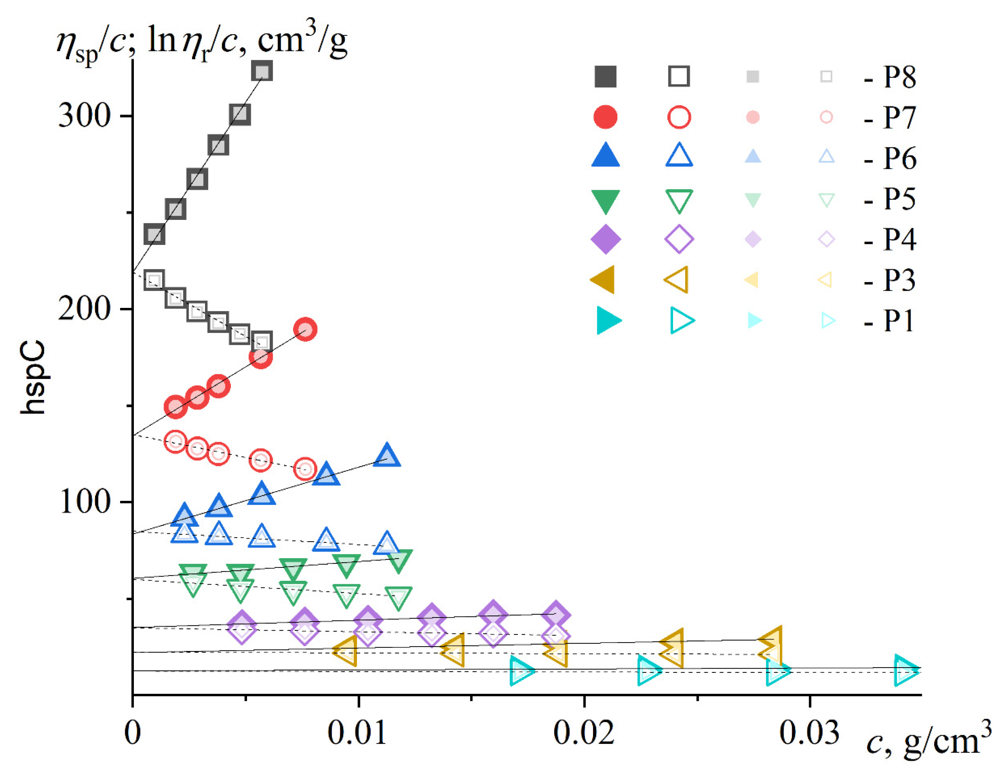
Figure 2.
The normalized distributions on sedimentation coefficient (a, b, c) and molar mass (d), which are resolved with implemented in Sedfit models: continuous distribution (a), direct fit of sedimentation boundary based on the least-squares analysis (b), continuous with general scaling law (c) and with extended Fujita approach (d). The exponent value used in and models is determined in Eq. (11). The presented distributions were resolved for the lowest measured concentrations ( g/dL) of pullulan solutions in DMF at 25°C. The notations next to the curves correspond to the sample notations in Table 1.
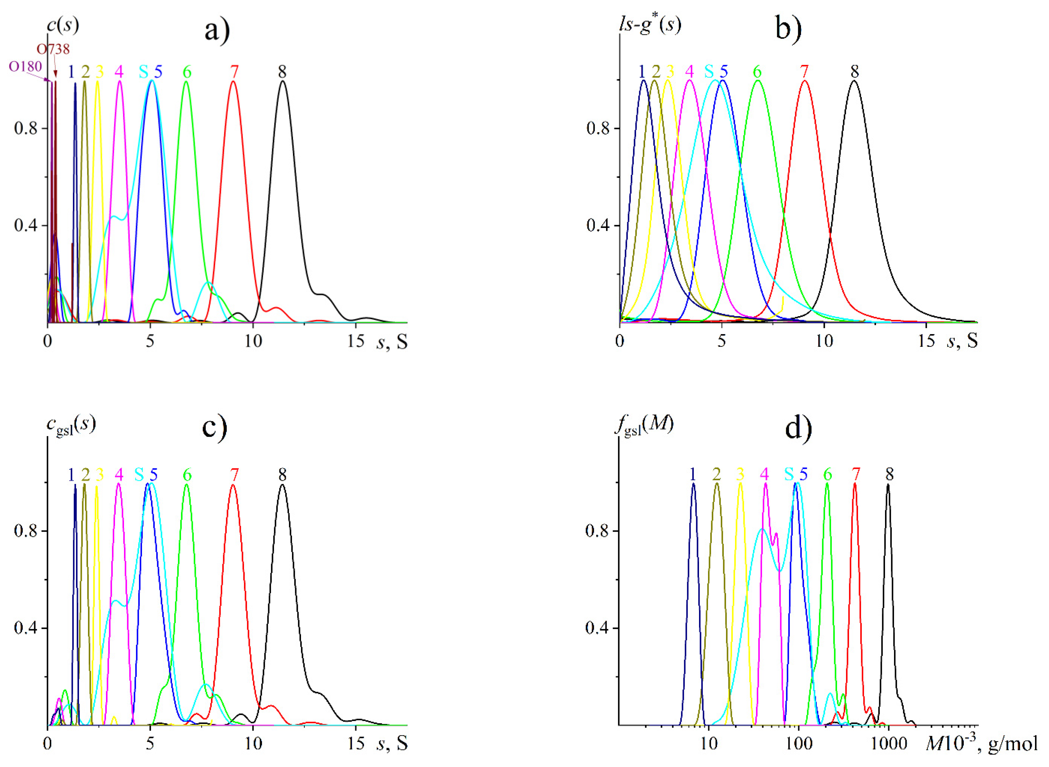
Figure 3.
The dispersion σ2 of the diffusion boundary with time t elapsed since the begining of the isothermal diffusion experiment for pullulan samples in DMF solutions at 25oC obtained with Tsvetkov polarizing diffusometer (a). Each succesive σ2(t) dataset is shifted along the Y-axis by 2.5∙10-3 cm2 except for the initial one for sample P8. The notations next to the lines correspond to the sample notations in Table 1. The inset (b) demonstrates diffusogramms for samples P1 and P8 taken at times , hours: 1.0(b1), 8.0(b2), 20(b3), 0.8 (b4) 2.0 (b5) and 3.8 (b6) elapsed since the experiments start. Arrows at inset (a) indicate datapoints resolved with corresponding diffusogramms presented at (b).
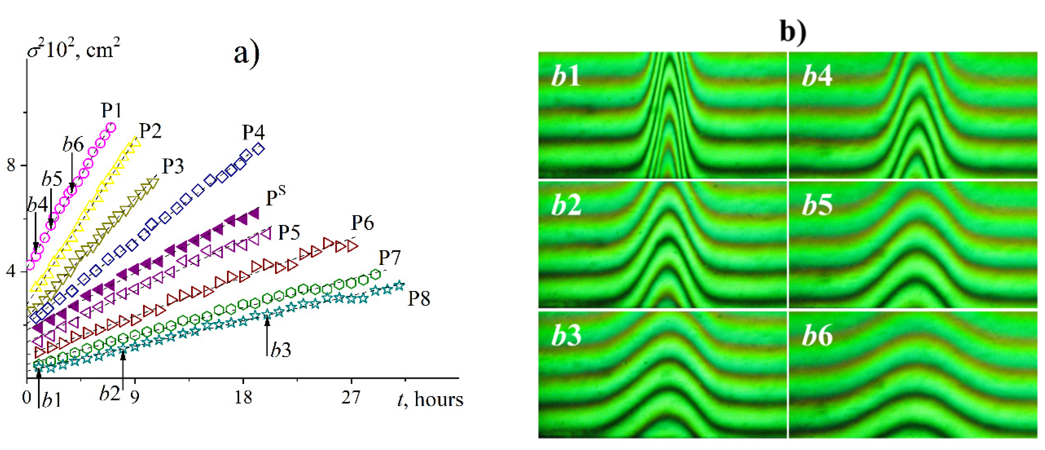
Figure 5.
The contour plot obtained by Monte Carlo calculations for wormlike chains with excluded-volume effects in dependence of Δ function values (error function Δ is represented as color gradient). The inset (a) presents the results for inhere studied pullulan in DMF at 25 °C and (b) demonstrates the results for summarized data on pullulan in H2O at 25 °C [21]. The data were treated with the latest Multi-HYDFIT version 3.0. The molar mass per unit chain length parameter is fixed at g/(mol cm).
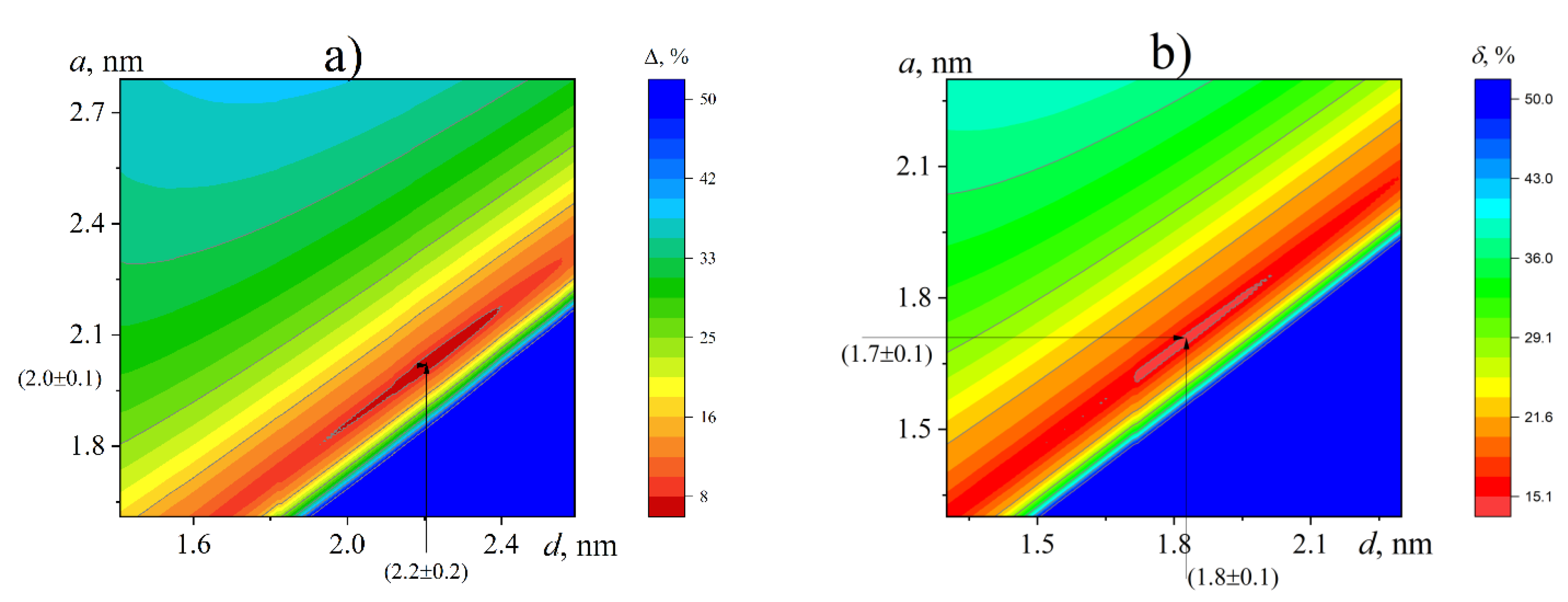
Table 1.
Supplier information on the sample properties (batch number, weight average molar mass (), polydispersity (Ɖ)) and the absolute molar mass obtained with sedimentation-diffusion analysis further in the study.
Table 1.
Supplier information on the sample properties (batch number, weight average molar mass (), polydispersity (Ɖ)) and the absolute molar mass obtained with sedimentation-diffusion analysis further in the study.
| Sample | Batch No. | , g/mol | Ɖ | , g/mol |
| P8 | 20908-3 | 788 | 1.23 | 640 |
| P7 | 20907-2 | 404 | 1.13 | 420 |
| P6 | 20906-2 | 212 | 1.13 | 200 |
| P5 | 20905-2 | 112 | 1.12 | 110 |
| PS* | P4516 | 100 | - | 94 |
| P4 | 20904-2 | 47.3 | 1.06 | 49 |
| P3 | 20903-2 | 22.8 | 1.07 | 23 |
| P2 | 20902-2 | 11.8 | 1.1 | 12 |
| P1 | 20901-2 | 5.9 | 1.09 | 7.2 |
| O730 | 20910-1 | 0.738 | 1 | 0.73 |
| O180 | 20909-1 | 0.180 | 1 | 0.21 |
* - The sample was purchased from Sigma-Aldrich.
Table 2.
The comparison of viscosity data obtained with Ostwald and Höppler viscometers. The intrinsic viscosity values are pre-averaged by results of Huggins and Kraemer approximation, Huggins (kH) and Kraemer () parameters, correspondingly.
Table 2.
The comparison of viscosity data obtained with Ostwald and Höppler viscometers. The intrinsic viscosity values are pre-averaged by results of Huggins and Kraemer approximation, Huggins (kH) and Kraemer () parameters, correspondingly.
| Sample | Ostwald viscometer | Höppler viscometer | ,% | ||||
| ,cm3/g | ,cm3/g | ||||||
| P8 | 213 | 0.36 | 0.14 | 219 | 0.37 | 0.14 | 2.8 |
| P7 | 133 | 0.4 | 0.13 | 135 | 0.40 | 0.13 | 1.5 |
| P6 | 84 | 0.47 | 0.11 | 84 | 0.50 | 0.10 | 0 |
| P5 | 59.2 | 0.28 | 0.18 | 60.2 | 0.24 | 0.21 | 1.7 |
| PS | 55 | 0.45 | 0.11 | 54 | 0.55 | 0.08 | -1.8 |
| P4 | 36.9 | 0.13 | 0.26 | 34.9 | 0.31 | 0.17 | -5.4 |
| P3 | 21.4 | 0.46 | 0.09 | 22.1 | 0.51 | 0.08 | 3.3 |
| P2 | 15.8 | 0.40 | 0.13 | 16.3 | 0.42 | 0.12 | 3.2 |
| P1 | 11.9 | 0.30 | 0.18 | 12.5 | 0.31 | 0.17 | 5 |
Table 3.
Hydrodynamic parameters, hydrodynamic invariants, molar masses and the number of statistic segments entering a polymer chain of pullulan samples in DMF at 25 °C.
Table 3.
Hydrodynamic parameters, hydrodynamic invariants, molar masses and the number of statistic segments entering a polymer chain of pullulan samples in DMF at 25 °C.
| Sample |
, cm3/g |
, cm2/s |
, s |
, cm3/g |
, mol-1/3 |
, cm2g/ (s2K mol1/3) |
, g/mol |
|
| P8 | 216 | 1.26 | 12.6 | 230 | 1.4 | 3.78 | 640 | 760 |
| P7 | 134 | 1.59 | 10.3 | 198 | 1.3 | 3.53 | 420 | 490 |
| P6 | 84 | 2.31 | 7.3 | 93 | 1.2 | 3.46 | 200 | 240 |
| P5 | 60 | 3.17 | 5.3 | 47 | 1.1 | 3.43 | 110 | 130 |
| PS | 55 | 3.47 | 5.1 | 60 | 1.2 | 3.49 | 94 | 110 |
| P4 | 36 | 4.73 | 3.6 | 25 | 1.0 | 3.32 | 49 | 58 |
| P3 | 22.2 | 6.86 | 2.5 | 27 | 1.1 | 3.20 | 23 | 28 |
| P2 | 16.1 | 9.37 | 1.8 | 3.18 | 12 | 15 | ||
| P1 | 12.2 | 12.27 | 1.38 | 3.17 | 7.2 | 9 | ||
| O730 | 5.9 | 34 | 0.39 | 3.22 | 0.73 | 0.9 | ||
| O180 | 5.5 | 62 | 0.2 | 3.77 | 0.21 | 0.3 |
Disclaimer/Publisher’s Note: The statements, opinions and data contained in all publications are solely those of the individual author(s) and contributor(s) and not of MDPI and/or the editor(s). MDPI and/or the editor(s) disclaim responsibility for any injury to people or property resulting from any ideas, methods, instructions or products referred to in the content. |
© 2024 by the authors. Licensee MDPI, Basel, Switzerland. This article is an open access article distributed under the terms and conditions of the Creative Commons Attribution (CC BY) license (https://creativecommons.org/licenses/by/4.0/).
Copyright: This open access article is published under a Creative Commons CC BY 4.0 license, which permit the free download, distribution, and reuse, provided that the author and preprint are cited in any reuse.


