
Submitted:
04 December 2024
Posted:
05 December 2024
You are already at the latest version
Abstract
Object detection in images is a fundamental component of many safety-critical systems, such as autonomous driving, video surveillance systems, and robotics. Adversarial patch attacks, which are easily implemented in the real world, provide effective counteraction to the object detection by state-of-the-art neural-based detectors. It poses a serious danger in various fields of activity. Existing defense methods against patch attacks are insufficiently effective, which underlines the need to develop new reliable solutions. In this manuscript, a new approach is proposed to increase the robustness of neural network systems to the input adversarial images. The proposed method, based on the anomaly localization, demonstrates high resistance to adversarial patch attacks while maintaining the high quality of the object detection. The results of the study demonstrate that the proposed method is promising for security of object detection systems improvement and threat of adversarial patch attacks counteraction.
Keywords:
adversarial patch attack
; robustness
; pedestrian detection
; deep convolutional neural network
1. Introduction
The development of automatic neural-based object detection in images has revolutionized the field of computer vision. Such systems are widely used in various fields of human activity, such as medicine [1], autonomous driving [2], video surveillance systems [3], analysis of urban changes [4], search and rescue operations [5], etc.
The ability of neural network systems to automatically identify and localize objects in images opens up new possibilities for automating tasks that previously required human participation. In this work, YOLOv3 is used as an object detector [6], because it is the most commonly used to solve the problem of quick multiple objects detection in a single image. This architecture has gained the greatest popularity for detecting objects in a video stream due to its speed. It is also worth noting that the source code and the weights of the model trained on the extensive MS COCO dataset [7] are publicly available. This factor increases the attractiveness of using this model to solve the problem of object detection and makes possible the comparison of the obtained results with the global level.
However, despite significant progress in the development and application of such systems, they face a serious threat from adversarial attacks [8]. In this paper, the white-box adversarial attacks are considered, since they are more effective than analogues of the black-box adversarial attacks [9]. Adversarial attacks can be divided into digital and physical implementations. Digital attacks directly manipulate the pixel values of the input images, which implies full access to the images. This type of attack can be implemented exclusively in digital form. Physical attacks introduce real-world objects into the environment that can affect the output of neural network systems. Real-world attacks, as a rule, are small fragments of images (patches), which are optimized in a digital environment before printing [10]. A prominent example of the implementation of a physical patch attack is the work [11], where the authors described the creation of an attack in a digital format that can be printed and applied in the real world. These patch attacks are aimed at deceiving the YOLOv3 system, pre-trained on the MS COCO dataset. The authors in [11] optimized adversarial patch attacks on the INRIA Person training dataset [12] to hide pedestrian. This dataset was originally created to solve pedestrian detection problems and contains images of people. The INRIA Person dataset consists of 614 images for training and 288 images for testing. An example of the patch noted above is shown in Figure 1.
Such attacks aimed at fooling neural networks can lead to critical errors in various areas. For example, in autonomous driving, the errors in object recognition can have catastrophic consequences. Adversarial patch attacks have demonstrated their effectiveness in misleading traffic sign classification systems [13], making the people invisible [11], or even hiding cars [14].
In this paper, a new method based on the idea of anomaly localization to reduce the impact of adversarial patch attacks on the object detector is proposed. The rest of this paper is structured as follows. Section 2 provides a brief overview of existing methods for removing adversarial patch attacks in images. The proposed method is described in detail in Section 3. The implementation details and evaluation metrics of the state-of-the-art defense methods are demonstrated in Section 4. Section 5 presents the results and discussions.
2. Related Work
One of the most popular methods to defend against adversarial attacks is adversarial training [15,16,17]. Such training increases the reliability of the model by augmenting the training data with adversarial images. A different approach was proposed in [18], in which, to defense against patch attacks, it was proposed to add a new class (namely, a class with an adversarial patch attack) and retrain the used object detector on a dataset enriched with adversarial images. In this way, the authors get an object detector that reveals both objects of interest and adversarial patches. Although adversarial training is the most effective strategy to improve the stability of the model at the moment, it inevitably requires time-consuming training. It is expensive to use for large-scale datasets and complex deep architectures, and the emergence of new adversarial attacks leads to the retraining of neural network systems. To avoid this problem, many researchers attempt to remove the adversarial attack before passing it to the object detector.
There is a number of papers concerning with the usage of adversarial training of external segmentator-based defenders. The PatchZero method [19] contains a segmentation model for detecting and removing adversarial patches. The Segment and Complete (SAC) method [20] consists of the well-proven U-Net architecture [21] for segmentation and removal of adversarial patches on input images. The authors [22] propose the Adversarial Pixel Masking (APM) method, in which the U-Net model is embedded in the general object detection pipeline. All these works contain an adversarial-trained external segmentator. However, detectors in these methods also remain vulnerable to new attacks. The external defense models need to be trained on a huge variety of new adversarial examples, which again leads to the need to allocate large resources for training.
The self-adaptive learned Universal Defense Filter (UDFilter) [23] consists of two modules: an adversarial patch generation module and a defense filter generation module. This method weakens the negative impact of adversarial patches by applying the obtained filter to the input image. In addition, the authors proposed a plug-and-play Joint Detection Strategy to maintain the performance of the model. The Patch-Agnostic Defense (PAD) method [24] is proposed to localize and remove adversarial patches without prior knowledge about the attack. The PAD includes the Segment Anything Model [25] for more accurate segmenting of the patches. The Local Gradient Smoothing (LGS) method [26] is independent on the patch attack, where the gradient of the input adversarial image is calculated to localize the adversarial patch. As it is known, the gradient allows to determine the image area containing high frequencies.
In recent years, some researchers have offered certified defensive methods against adversarial patches. For example, the Detectorguard method [27] detects the presence of attacks without removing them. It may lead to the loss of model functionality during the attack. The Objectseeker method [28] removes parts of the input image. After that the Objectseeker looks for at least one split of the input image in which the adversarial patch does not affect the detection of objects. However, when processing attack scenarios with a large number of patches, this method may fail.
An analysis of the related work shows that there is an unsolved problem: most of the existing state-of-the-art methods for removing adversarial patch attacks require resource-intensive retraining when new adversarial attacks appear. This limits the applicability of existing methods to multiple variations of attacks. The proposed study in this paper is aimed at solving this problem.
3. Proposed Method
The proposed method is based on the idea of detecting and removing anomalies in the input images. The differences between the benign image (image without the addition of adversarial attacks) and adversarial image (image with the addition of adversarial attacks) are considered as anomalies in this work. A simplified scheme of the proposed method is shown in Figure 2.
The proposed algorithm is represented by a sequence of logical blocks, each of which implements a specific task. The Deep Convolutional Neural Network (DCNN) generates an approximate benign image based on the input image. The Calculating Maximum Error block calculates the difference between the input and generated images. The Localizing Anomalous Fragments block aims to extract anomalous fragments from the input images, and the Clustering & Processing block groups the anomalies obtained in the previous step into clusters to process them further. The anomaly map resulting from these blocks, which highlights areas with anomalies, is sent to the Applying Anormaly Map block to remove anomalous areas from the input image. The result of applying the anomaly map is sent to the object detector. A more detailed description of each block from Figure 2 is shown below.
3.1. Deep Convolutional Neural Network for Benign Image Reconstruction
To solve the problem of the absence of a priori known benign images, in this paper it is proposed to generate an approximately benign image based on the input one.
Currently, the AnoGAN [29] addresses the problem of neural network-based image reconstruction. However, the neural network architecture of AnoGAN is quite simple and is capable of generating images that contain, for example, simple texture patterns and images of objects occupying a larger area in the image. It is worth noting that AnoGAN demonstrates high performance in solving the task of localizing anomalous areas in medical images.
However, complex data is used in the present study, i.e., images with complex backgrounds and containing various multiple elements (people, road signs, vehicles). Also, these images do not always have high quality. Thus, it is necessary to use a deep neural network architecture to reconstruct the complex images, which leads to challenging training due to limited data.
To address this issue, it is proposed to use a Deep Convolutional Neural Network (DCNN in Figure 2), which, like in [29], is unsupervised trained exclusively on clean images. This approach allows to obtain a system that lacks knowledge of the attack, which increases its applicability to various attack variations.
The proposed DCNN architecture is inspired by the idea of an autoencoder [30]. So, the used DCNN consists of two parts: an encoder, which addresses the task of efficiently compressing the input data; and a decoder, which aims to reconstruct the original image from the compressed data. This aspect allows decreasing content of the adversarial attack at the encoder stage and reconstructing the image from the compressed data with significant attack weakening. Additionally, to preliminary decrease the attack, the DCNN is trained to convert a grayscale image to its colored version.
The Figure 3(a) shows a simplified diagram of the used DCNN. The fully convolutional part of the deep neural network’s architecture, ResNet50 [31], is used as an encoder. Such neural network consists of five blocks, each of which reduces the spatial dimensions of the input image by half. As in the paper [31], the conv64 block consists of sequentially connected convolution layer with 64 output filters, a BatchNormalization layer, a ReLU activation layer, and a MaxPooling layer that reduces the spatial resolution by half. The resconvU block is residual block with U output filters.
As a decoder, it is proposed to use five sequentially connected blocks, each of which multiplies the spatial dimensions of the input data by two. The deconvU block is proposed to consist of sequentially connected transposed convolution layers with U output filters, a BatchNormalization layer, and a ReLU activation layer (see Figure 3(b)).
The mean squared error (MSE) function is used to calculate the difference between the original color image and the generated image. MSE is then used as the loss function for training this DCNN.
Thus, the proposed method for benign image reconstruction doesn’t require labeling data, which makes this approach more flexible for solving multiple tasks. It can also be seen that the proposed DCNN is quite simple, which makes it quite easy to reproduce this case. However, it is worth noting that the overall performance of the whole proposed method depends on the chosen DCNN architecture.
3.2. Calculating Maximum Error
Let’s denote the source color image as , and the generated benign color image as . The spatial dimensions of the images are H and W pixels in height and width, respectively; the number of color channels is 3, which corresponds to the RGB-format. The brightness value of the image pixels is normalized to the maximum possible pixel brightness, i.e. the values of X and Y vary in the range from 0.0 to 1.0. In this paper, the following expression is used to calculate the error value, representing the difference between the original and generated images:
where i, j are the indexes of the row and column of images, respectively; color is the index of the color channel of the image, which can take the values 0, 1 and 2 for the red, green and blue channels, respectively; is the error map between the source and generated benign images. Maximizing the error value for the color component allows to reduce the number of parameters for subsequent processing, as well as to reduce information about the color reconstruction error. Figure 4 shows an example of an error map obtained by expression (1) for clean and adversarial images.
The areas with a patch attack that can be considered anomalies are visually highlighted in Figure 4(d), i.e. the values of the error map are relatively high. It’s also worth noting that Figure 4(c) shows errors in reconstructed benign image, which should not be highlighted as anomalies. For these purposes, an anomalous fragments localizing algorithm has been developed. This algorithm is described in the following section.
3.3. Localizing Anomalous Fragments
A simplified scheme of the operations sequence in the Localizing Anomalous Fragments block is shown in Figure 5.
In this paper, in order to identify anomalous areas, the error map is split into fragments by a sliding window of size with a step according to the following expression:
where is the result of splitting the error map into fragments; is the error map from expression (1); r and c are the indexes of fragments in height and width, respectively; and are the indexes in height and width of each fragment, respectively.
Figure 4(d) shows that the error magnitude changes sharply at the patch attack location. The magnitude changes are smaller in the fragments without patch attack. Rich information about the change in errors within the fragments can be obtained from the histogram. Thus, for further processing of the error map, the values of the error map’s fragments transform into the histograms. The described step can be formulated as the following expression:
where is the result of calculating the histograms of all fragments; B is the number of bins to build a histogram; is the index of the bins; histogram(·) is the operator for calculating the histogram. The obtained histograms are fed into the Isolation Forest algorithm [32], which identifies fragments with anomalous histograms. The Isolation Forest algorithm is a powerful tool for identifying anomalous data. Thus, a sharp change in the histograms of fragments where the patch attack is located, relative to the other histograms, can be considered as anomalous behavior. This anomalous behavior is detected by the Isolation Forest algorithm. This stage can be represented by the following formula:
where is the obtained anomalous fragments map, which is a binary matrix with spatial dimensions such that
A median filter is applied to remove scattered fragments marked as anomalous while simultaneously grouping dense anomalous fragments. Figure 6 shows a result of the anomalous fragment localization algorithm for the clean and adversarial images mentioned in Figure 4(a) and (b), respectively.
The algorithm described above highlights anomalous fragments, as can be seen from Figure 6. However, due to the lack of a priori knowledge about attacks (their presence, number, size, and shape), it is necessary to post-process the obtained information. The post-processing algorithm is described in the next subsection.
3.4. Clustering and Processing of the Anomalies
A simplified scheme of the proposed Clustering & Processing block is presented in Figure 7.
The coordinates of anomalous fragments obtained in the previous stage are fed as input data into the DBSCAN clustering algorithm [33]. The DBSCAN algorithm solves the problem of grouping closely located anomalous fragments and removing randomly marked anomalous fragments. The DBSCAN clustering algorithm allows for finding groups of densely located points without prior knowledge of the number and shapes of these groups, and, at the same time, the DBSCAN algorithm is robust to noise outliers, which may occur in the case of insufficiently accurate image generation in the DCNN, for example. As a result of the clustering stage, L clusters are obtained, and each cluster contains a different number of fragments belonging to a specific cluster.
The next stage is calculating the Pearson correlation coefficient [34] between the histograms of fragments belonging to the cluster with index l and the histograms of neighbor fragments around the cluster with index l. The correlation coefficient is a scalar that indicates the level of relationship between two variables. The correlation coefficient is convenient due to its clear interpretation: it approaches 1.0 if the compared data are very similar; it approaches 0.0 if the compared data are completely different.
At this stage, the histograms of the fragments from the source image X are analyzed. That is, initially, the source image X is split into fragments according to the same rule as in the block for localizing anomalous fragments:
where is the result of splitting the source image X into fragments by sliding window with size and stride , color is the index of the color channel. Further, as in the localizing anomalous fragments block, a histogram is built for each fragment according to the following rule:
where is the result of calculating the histograms of all fragments in , is the number of bins to build a histogram, is the index of the bins.
The result of the Calculating correlations algorithm for each cluster with index l is a two-dimensional matrix, each element of which is calculated as follows:
where and are the sets of the histograms, built from the source image’s fragments, identified as anomalous and normal at the localizing anomalous fragments block, respectively; A is the number of anomalous fragments; N is the number of normal fragments; is the index of the anomalous fragment in the cluster with index l; is the index of the normal fragment, which is in the neighborhood around the cluster with index l. As a result of executing this algorithm, a set of two-dimensional Pearson correlation coefficient matrices for each cluster is obtained.
Given that the adversarial patch attack represents a local perturbation, it can be logically concluded that the image around the adversarial patch attack is semantically different from the image of the patch attack itself (these two images don’t correlate).
It can be concluded that the histograms of adversarial patch attacks should differ significantly from the histograms of the neighborhood around this patch attack. Since the correlation coefficient indicates the level of similarity, the correlation coefficient between the adversarial patch attack and the neighborhood around this attack should be low due to the semantic independence of the patch attack and its neighborhood. Thus, for each cluster, the median value of the Pearson correlation coefficient is calculated according to the following rules:
where and are the operations that calculate median value along a certain variable. The obtained median value of the Pearson correlation coefficient is compared with the empirically established threshold. If this value is lower than the threshold, the cluster is considered anomalous.
In this paper, to obtain an anomaly map M (see Figure 2), the pixel brightness values from an anomalous cluster are extracted from the source image X and their average value is calculated. The average pixel value in the anomalous cluster is assigned to pixels in the anomaly map M at the location of this cluster.
Figure 8 shows examples of anomaly maps for the clean and adversarial images mentioned in Figure 4 (a) and (b), respectively. The maps are obtained as a result of the clustering and processing algorithm.
Figure 8 shows that the algorithm described above processes the data extracted from the localizing anomalous fragments block and makes decision to identify this data as anomaly or not.
3.5. Applying an Anomaly Map to an Image
The obtained anomaly map must be applied to the source image X as follows:
The expression (11) allows to save the source image and, at the same time, to hide anomalous areas. The obtained image is sent to the attacked object detection system as input for subsequent objects of interest detection. Thus, the localized adversarial patch attacks in the image are replaced by uniformly colored figures, which reduce the strength of the attacks to a minimum, thereby minimizing their impact on the object detection system.
4. Evaluation
4.1. Implementation Details
The pre-trained on MS COCO object detector YOLOv3 [6] is used as an object detector.
The DCNN proposed in Section 4.1 was trained using only the part of the MS COCO training dataset that has images containing people. Let’s name this dataset as MS COCO Person. The volume of the MS COCO Person training dataset is 64115 images. DCNN was trained for 48 epochs; the batch size is 4. The learning rate first warms up to a value of 1e-4 in 500 iterations, after which it decreases to a value of 1e-5 according to the cosine schedule. The optimizer is Adam with and .
In section 4.3, a sliding window has a size F=8 and a stride S=8.
The Isolation Forest and DBSCAN algorithms used in Section 4.4 are implemented in the Python programming language using the scikit-learn package [35]. The DBSCAN algorithm requires setting two parameters: the minimum number of points is 9 and the size of the neighborhood is to obtain dense clusters. The remaining parameters for the Isolation Forest and DBSCAN algorithms are taken by default from the scikit-learn package. The threshold of the median Pearson coefficient in Section 4.4 is 0.1.
4.2. Experimental Results
The most popular methods aimed at defending pedestrian detectors from adversarial patch attacks, namely the PAD [24] and the SAC [20], are used for comparison. It is also worth noting that the implementations of these methods are publicly available, which makes it possible to compare them using the same test dataset and object detector.
Initially, the SAC method was applied to detect the digital patch attack projected gradient descent (PGD) [36], using self-training for this purpose. However, the analysis of the effectiveness of the SAC method on patch attack images from work [11] did not yield positive results. For this experiment, the SAC method was trained on the MS COCO Person training dataset with applied real-world adversarial patch attacks from [11]. The other settings for this method remained unchanged.
Table 1 presents a comparative analysis of the proposed and the existing patch attacks defense methods. The object detection quality metrics mAP [7] were calculated on the INRIA-Person [12] test dataset without adding attacks (Clean column) and with adding attacks (Adversarial column).
The results presented in Table 1 show that the proposed method outperforms the state-of-the-art SAC and PAD methods.
5. Results and Discussion
The method for increasing the robustness of neural-based pedestrian detector is presented in this paper. The method aims to adversarial patch attacks counteraction by localizing anomalies in the images. The proposed method consists of a deep convolutional neural network, an anomaly localizing algorithm, a clustering and anomaly processing algorithm.
The DCNN generates the image that is close to the input image but with reduced content of the adversarial attack. This aspect excludes the need to retrain the object detector when new examples of adversarial patch attacks appear.
The proposed method utilizes rich statistical information obtained from the local histograms of error map and input images. The combination of the aforementioned conventional data processing algorithms represents a powerful tool for counteracting the local anomalous perturbations in images.
This paper also demonstrates that even a relatively simple DCNN architecture, combined with the proposed anomaly localizing and post-processing algorithm, outperforms the state-of-the-art methods, namely, SAC and PAD. The idea of using a lightweight deep convolutional neural network and conventional machine learning methods allows for the effective processing of complex images without high computational costs.
The proposed method also doesn’t use any knowledge about patch attacks and doesn’t require retraining the object detector, thus being computationally efficient. It makes the proposed method suitable for a variety of applications, which utilize relatively simple and cheap hardware.
Author Contributions
Conceptualization, O.I. and M.T.; methodology, M.T., O.I. and V.Z.; validation, O.I.; formal analysis, M.T., O.I. and V.Z.; investigation, O.I.; writing—original draft preparation, O.I.; writing—review and editing, M.T. and V.Z; supervision, M.T.. All authors have read and agreed to the published version of the manuscript.
Funding
This research received no external funding.
Institutional Review Board Statement
Not applicable.
Informed Consent Statement
Not applicable.
Data Availability Statement
Publicly available datasets were used in this study.
Conflicts of Interest
The authors declare no conflict of interest.
References
- Galić, I.; Habijan, M.; Leventić, H.; Romić, K. Machine learning empowering personalized medicine: A comprehensive review of medical image analysis methods. Electronics 2023, 12, 4411. [Google Scholar] [CrossRef]
- Feng, D.; Harakeh, A.; Waslander, S.L.; Dietmayer, K. A review and comparative study on probabilistic object detection in autonomous driving. IEEE Transactions on Intelligent Transportation Systems 2021, 23, 9961–9980. [Google Scholar] [CrossRef]
- Luna, E.; San Miguel, J.C.; Ortego, D.; Martínez, J.M. Abandoned object detection in video-surveillance: survey and comparison. Sensors 2018, 18, 4290. [Google Scholar] [CrossRef] [PubMed]
- Li, Z.; Shen, H.; Cheng, Q.; Liu, Y.; You, S.; He, Z. Deep learning based cloud detection for medium and high resolution remote sensing images of different sensors. ISPRS Journal of Photogrammetry and Remote Sensing 2019, 150, 197–212. [Google Scholar] [CrossRef]
- Bejiga, M.B.; Zeggada, A.; Nouffidj, A.; Melgani, F. A convolutional neural network approach for assisting avalanche search and rescue operations with UAV imagery. Remote Sensing 2017, 9, 100. [Google Scholar] [CrossRef]
- Farhadi, A.; Redmon, J. Yolov3: An incremental improvement. In Proceedings of the Computer vision and pattern recognition. Springer Berlin/Heidelberg, Germany, Vol. 1804; 2018; p. 1. [Google Scholar]
- Lin, T.Y.; Maire, M.; Belongie, S.; Hays, J.; Perona, P.; Ramanan, D.; Dollár, P.; Zitnick, C.L. Microsoft coco: Common objects in context. In Proceedings of the Computer Vision–ECCV 2014: 13th European Conference, Zurich, Switzerland, 2014, Proceedings, Part V 13. Springer, 2014, September 6-12; pp. 740–755.
- Goodfellow, I.J.; Shlens, J.; Szegedy, C. Explaining and harnessing adversarial examples. arXiv preprint arXiv:1412.6572 2014. arXiv:1412.6572 2014.
- Wang, Y.; Liu, J.; Chang, X.; Rodríguez, R.J.; Wang, J. Di-aa: An interpretable white-box attack for fooling deep neural networks. Information Sciences 2022, 610, 14–32. [Google Scholar] [CrossRef]
- Wang, D.; Yao, W.; Jiang, T.; Tang, G.; Chen, X. A survey on physical adversarial attack in computer vision. arXiv preprint arXiv:2209.14262, arXiv:2209.14262 2022.
- Thys, S.; Van Ranst, W.; Goedemé, T. Fooling automated surveillance cameras: adversarial patches to attack person detection. In Proceedings of the Proceedings of the IEEE/CVF conference on computer vision and pattern recognition workshops, 2019, pp.; pp. 0–0.
- Dalal, N.; Triggs, B. Histograms of oriented gradients for human detection. In Proceedings of the 2005 IEEE computer society conference on computer vision and pattern recognition (CVPR’05). Ieee, Vol. 1; 2005; pp. 886–893. [Google Scholar]
- Wei, X.; Guo, Y.; Yu, J. Adversarial sticker: A stealthy attack method in the physical world. IEEE Transactions on Pattern Analysis and Machine Intelligence 2022, 45, 2711–2725. [Google Scholar] [CrossRef] [PubMed]
- Du, A.; Chen, B.; Chin, T.J.; Law, Y.W.; Sasdelli, M.; Rajasegaran, R.; Campbell, D. Physical adversarial attacks on an aerial imagery object detector. In Proceedings of the Proceedings of the IEEE/CVF Winter Conference on Applications of Computer Vision, 2022, pp.; pp. 1796–1806.
- Zhao, W.; Alwidian, S.; Mahmoud, Q.H. Adversarial training methods for deep learning: A systematic review. Algorithms 2022, 15, 283. [Google Scholar] [CrossRef]
- Rao, S.; Stutz, D.; Schiele, B. Adversarial training against location-optimized adversarial patches. In Proceedings of the European conference on computer vision. Springer; 2020; pp. 429–448. [Google Scholar]
- Wu, T.; Tong, L.; Vorobeychik, Y. Defending against physically realizable attacks on image classification. arXiv preprint arXiv:1909.09552 2019. arXiv:1909.09552 2019.
- Ji, N.; Feng, Y.; Xie, H.; Xiang, X.; Liu, N. Adversarial yolo: Defense human detection patch attacks via detecting adversarial patches. arXiv preprint arXiv:2103.08860 2021. arXiv:2103.08860 2021.
- Xu, K.; Xiao, Y.; Zheng, Z.; Cai, K.; Nevatia, R. Patchzero: Defending against adversarial patch attacks by detecting and zeroing the patch. In Proceedings of the Proceedings of the IEEE/CVF Winter Conference on Applications of Computer Vision, 2023, pp.; pp. 4632–4641.
- Liu, J.; Levine, A.; Lau, C.P.; Chellappa, R.; Feizi, S. Segment and complete: Defending object detectors against adversarial patch attacks with robust patch detection. In Proceedings of the Proceedings of the IEEE/CVF Conference on Computer Vision and Pattern Recognition, 2022, pp.; pp. 14973–14982.
- Ronneberger, O.; Fischer, P.; Brox, T. U-net: Convolutional networks for biomedical image segmentation. In Proceedings of the Medical image computing and computer-assisted intervention–MICCAI 2015: 18th international conference, Munich, Germany, 2015, proceedings, part III 18. Springer, 2015, October 5-9; pp. 234–241.
- Chiang, P.H.; Chan, C.S.; Wu, S.H. Adversarial pixel masking: A defense against physical attacks for pre-trained object detectors. In Proceedings of the Proceedings of the 29th ACM international conference on multimedia, 2021, pp.; pp. 1856–1865.
- Mao, Z.; Chen, S.; Miao, Z.; Li, H.; Xia, B.; Cai, J.; Yuan, W.; You, X. Enhancing robustness of person detection: A universal defense filter against adversarial patch attacks. Computers & Security 2024, 146, 104066. [Google Scholar]
- Jing, L.; Wang, R.; Ren, W.; Dong, X.; Zou, C. PAD: Patch-Agnostic Defense against Adversarial Patch Attacks. In Proceedings of the Proceedings of the IEEE/CVF Conference on Computer Vision and Pattern Recognition, 2024, pp.; pp. 24472–24481.
- Kirillov, A.; Mintun, E.; Ravi, N.; Mao, H.; Rolland, C.; Gustafson, L.; Xiao, T.; Whitehead, S.; Berg, A.C.; Lo, W.Y.; et al. Segment anything. In Proceedings of the Proceedings of the IEEE/CVF International Conference on Computer Vision, 2023, pp.; pp. 4015–4026.
- Naseer, M.; Khan, S.; Porikli, F. Local gradients smoothing: Defense against localized adversarial attacks. In Proceedings of the 2019 IEEE Winter Conference on Applications of Computer Vision (WACV). IEEE; 2019; pp. 1300–1307. [Google Scholar]
- Xiang, C.; Mittal, P. Detectorguard: Provably securing object detectors against localized patch hiding attacks. In Proceedings of the Proceedings of the 2021 ACM SIGSAC Conference on Computer and Communications Security, 2021, pp.; pp. 3177–3196.
- Xiang, C.; Valtchanov, A.; Mahloujifar, S.; Mittal, P. Objectseeker: Certifiably robust object detection against patch hiding attacks via patch-agnostic masking. In Proceedings of the 2023 IEEE Symposium on Security and Privacy (SP). IEEE; 2023; pp. 1329–1347. [Google Scholar]
- Schlegl, T.; Seeböck, P.; Waldstein, S.M.; Schmidt-Erfurth, U.; Langs, G. Unsupervised anomaly detection with generative adversarial networks to guide marker discovery. In Proceedings of the International conference on information processing in medical imaging. Springer; 2017; pp. 146–157. [Google Scholar]
- Li, P.; Pei, Y.; Li, J. A comprehensive survey on design and application of autoencoder in deep learning. Applied Soft Computing 2023, 138, 110176. [Google Scholar] [CrossRef]
- He, K.; Zhang, X.; Ren, S.; Sun, J. Deep residual learning for image recognition. In Proceedings of the Proceedings of the IEEE conference on computer vision and pattern recognition, 2016, pp.; pp. 770–778.
- Liu, F.T.; Ting, K.M.; Zhou, Z.H. Isolation forest. In Proceedings of the 2008 eighth ieee international conference on data mining. IEEE; 2008; pp. 413–422. [Google Scholar]
- Ester, M.; Kriegel, H.P.; Sander, J.; Xu, X.; et al. A density-based algorithm for discovering clusters in large spatial databases with noise. In Proceedings of the kdd, 1996, Vol. 96, pp. 226–231.
- Cohen, I.; Huang, Y.; Chen, J.; Benesty, J.; Benesty, J.; Chen, J.; Huang, Y.; Cohen, I. Pearson correlation coefficient. Noise reduction in speech processing 2009, pp. 1–4.
- Pedregosa, F.; Varoquaux, G.; Gramfort, A.; Michel, V.; Thirion, B.; Grisel, O.; Blondel, M.; Prettenhofer, P.; Weiss, R.; Dubourg, V.; et al. Scikit-learn: Machine learning in Python. the Journal of machine Learning research 2011, 12, 2825–2830. [Google Scholar]
- Mądry, A.; Makelov, A.; Schmidt, L.; Tsipras, D.; Vladu, A. Towards deep learning models resistant to adversarial attacks. stat 2017, 1050. [Google Scholar]
Figure 1.
Example of the adversarial patch attack, generated by minimizing the object detector’s objectness score. The image is taken from [11].
Figure 1.
Example of the adversarial patch attack, generated by minimizing the object detector’s objectness score. The image is taken from [11].
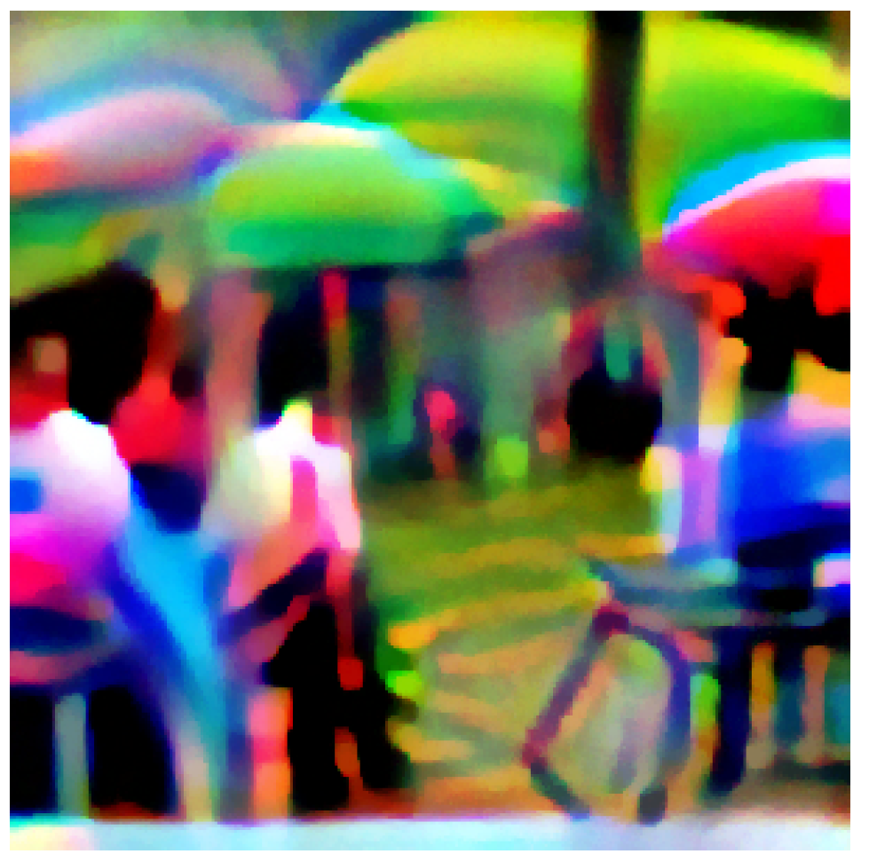
Figure 2.
Simplified scheme of the proposed method.
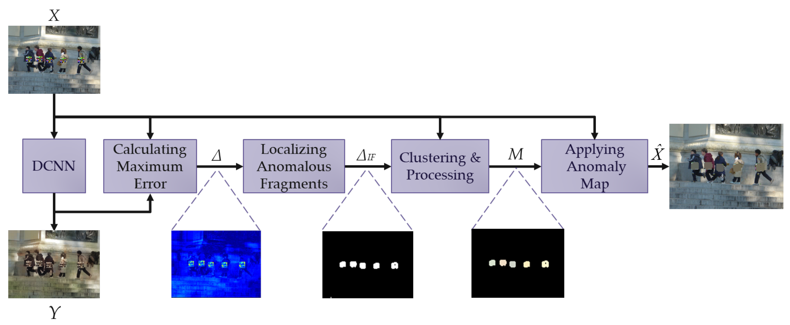
Figure 3.
Simplified diagram of the used DCNN (a). Simplified diagram of the decoder’s block (b).
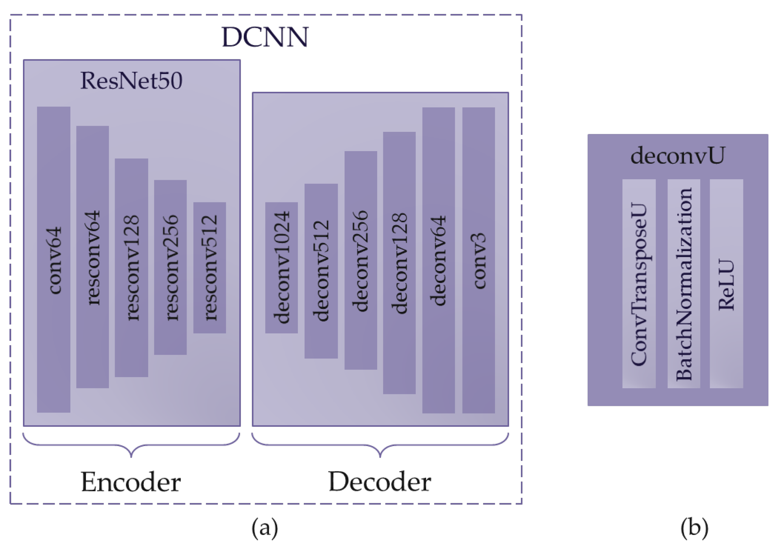
Figure 4.
Example of a benign image (a) and its corresponding error map (c); example of an adversarial image (b) and its corresponding error map (d).
Figure 4.
Example of a benign image (a) and its corresponding error map (c); example of an adversarial image (b) and its corresponding error map (d).
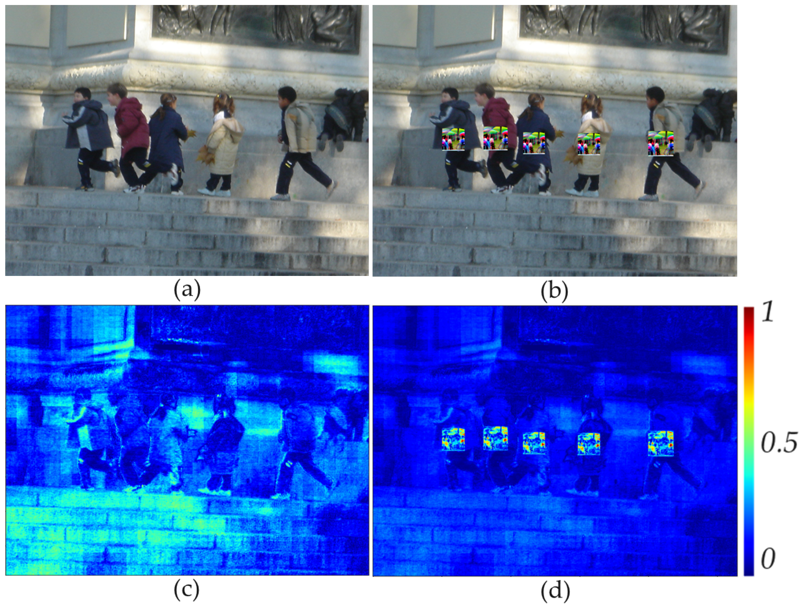
Figure 5.
Simplified scheme of the Localizing Anomalous Fragments block.
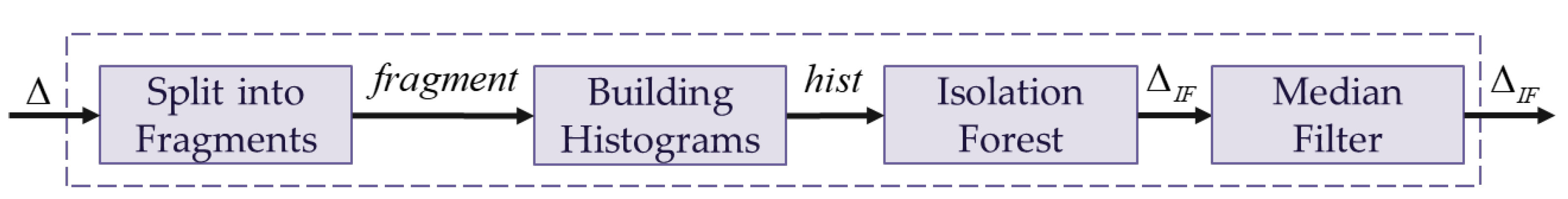
Figure 6.
Examples of anomalous fragment maps for a benign image (a) and for an adversarial image (b).
Figure 6.
Examples of anomalous fragment maps for a benign image (a) and for an adversarial image (b).
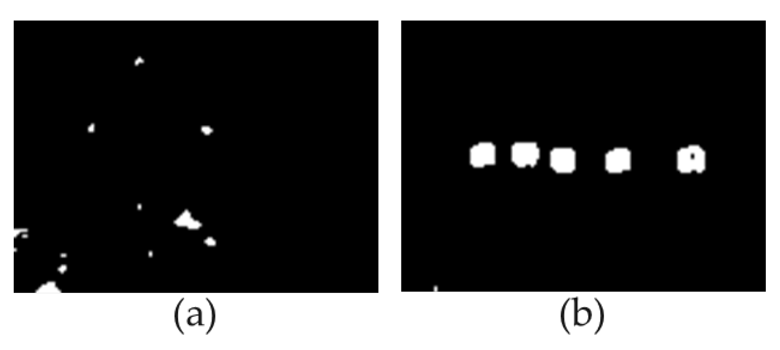
Figure 7.
Simplified scheme of the proposed Clustering & Processing block.
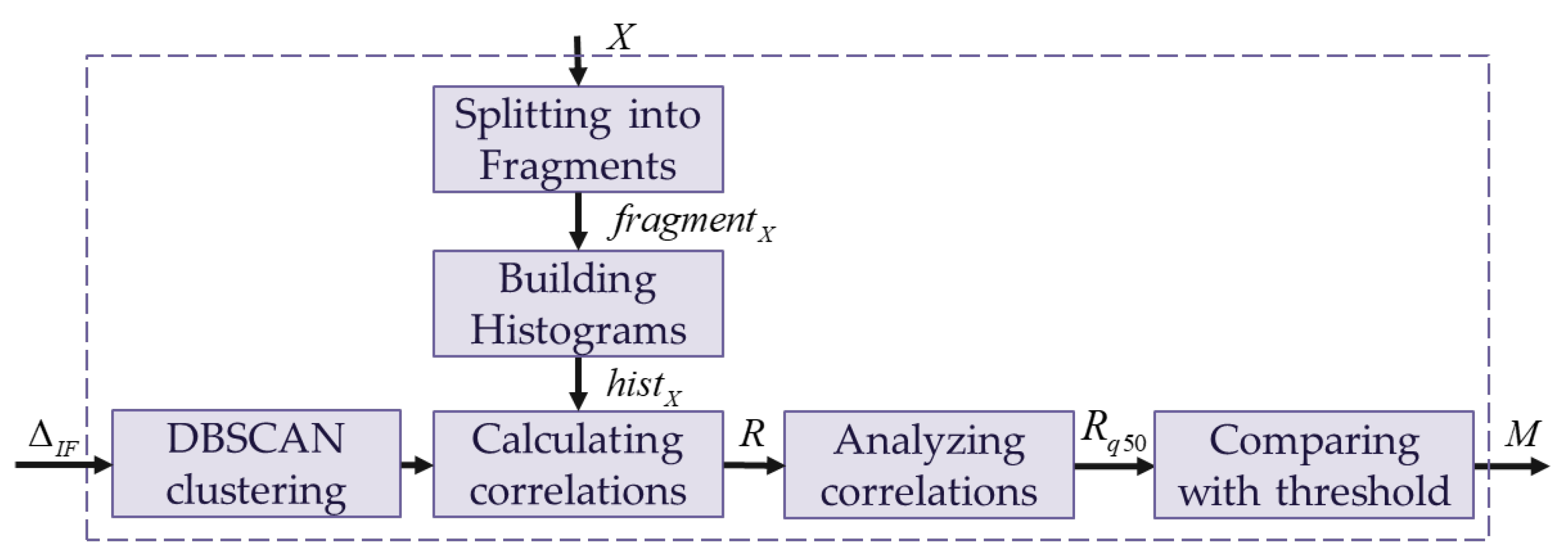
Figure 8.
Examples of anomaly maps for a benign image (a) and for an adversarial image (b).
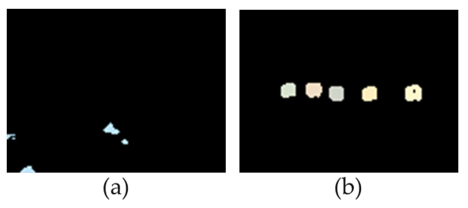

Table 1.
mAP(%) under adversarial patch attack [11] for different defense methods. The best performance is bolded, and the suboptimal performance is underlined.
Disclaimer/Publisher’s Note: The statements, opinions and data contained in all publications are solely those of the individual author(s) and contributor(s) and not of MDPI and/or the editor(s). MDPI and/or the editor(s) disclaim responsibility for any injury to people or property resulting from any ideas, methods, instructions or products referred to in the content. |
© 2024 by the authors. Licensee MDPI, Basel, Switzerland. This article is an open access article distributed under the terms and conditions of the Creative Commons Attribution (CC BY) license (http://creativecommons.org/licenses/by/4.0/).
Copyright: This open access article is published under a Creative Commons CC BY 4.0 license, which permit the free download, distribution, and reuse, provided that the author and preprint are cited in any reuse.


