
Submitted:
02 December 2024
Posted:
02 December 2024
You are already at the latest version
Abstract
Customers arrive at a single server queue with a finite sequence M of orbits for retrial customers based on the number of retrials made by each customer. Of these M orbits, the first M−1 are of finite capacities and the last one ( marked M) is of infinite capacity. Primary arrivals who are unable to access the server upon arrival, go to an orbit of finite capacity. From this orbit customers retry; those who fail to access the server join a second orbit of size larger than the first one and retry to access the server. Finally, they join the Mth orbit (after M−1 repeated trials). Retrials from all the orbits are assumed to be linear. Retrials occur from the Mth orbit and if those were unsuccessful, each customer will come back to the Mth orbit itself with probability q whereas with probability 1−q, leaves the system. Also after each service completion epoch, the server goes in search of customers from the Mth orbit with probability p. With probability 1−p the server remains idle. Steady-state analysis has been done. Various measures of performance are calculated. We analyze this retrial queuing model graphically as well as numerically. We also analyze the model for the optimum value of search probability. Some probability distributions of interest related to the model, have been derived.
Keywords:
Retrial Queue
; Multi-Orbits
; Transfer of orbital customers to service station
; Abandonment of last orbit
; Search
MSC: 60J28; 60K25; 90B05; 90B22
1. Introduction
The Retrial Queueing (RTQ) model under consideration is a single server model with a finite number of orbits arranged in hierarchical order, labeled as , and arranged in that order. Their capacities are respectively and unlimited for the orbit-M. Further, the retrial rate of customers from these orbits has individual rates , , ..., . These two facts together almost ensure minimum loss of customers, consequent to failed retrials, for a reason to be indicated in the descriptions to follow. If the server is busy at the time of arrival of a primary customer he/she will join the first orbit. Retrials are made from the first orbit and if those are unsuccessful, customers move to the next orbit and so on until they reach the last orbit. All the orbits except orbit-M are of finite capacity. The last orbit, orbit-M has infinite capacity and the customers in that orbit may either return to the same orbit or leaves the system forever, after each unsuccessful retrial attempt. Retrials from all the orbits follow linear retrial policy. Thus the model under consideration takes into account the impatience of customers in such queueing systems. On completion of service, the server transfers a customer from orbit M with probability p for the next service or stays idle with probability . The time taken for transfer is negligible. Thus, customers in that orbit (who have already completed at least retrials) will get higher priority over all customers from other orbits and also the primary arrivals.
In the mathematical modeling of real-life problems, the theory of retrial queues plays a pivotal role. The monograph by Falin and Templeton [11], gives an introduction to the theory of retrial queues. Over the years, the theory of retrial queues has been developing and the literature covers various fields in which the theory can practically be applicable. The book by Artalejo and Gomez-Corral [4] includes comprehensive coverage of techniques for the computational analysis of retrial queues. It includes motivating examples in telephone and computer networks and a comparative analysis of the retrial queues versus standard queues with waiting lines and queues with losses. A modern treatment for the study of retrial queues can be seen in the books by Dudin et al. [9] and Chakravarthy [5,6]. Detailed and classified bibliography of articles on retrial queues can be found in [1,2]. The survey on retrial queues in [13,20] includes literature with algorithmic and computational aspects of retrial queues.
When we analyze most of the retrial queueing models, we can find that the server remains idle even if there are customers in the corresponding orbit/orbits. This happens just because of the fact that the retrying customers are unaware of the status of the server. Retrying customers will succeed in getting service only if the server is idle at the retrying epoch. To overcome the difficulties posed by such situations and to improve the utilization of the server the concept of orbital search in negligible time to the server at the end of a service completion epoch was introduced. In the classical queueing models the concept of searching of customers was introduced by Neuts and Ramalhoto [16]. It was extended to the case of retrial queues in 2002 by Artalejo et al. in [3]. Krishnamoorthy et.al.[14] extended the search mechanism to a queueing model in which the blocked customers leave the system forever. Orbital search in a wider sense is used in [7,8,12,15]. In these papers, the authors assume different distributions for the search time of customers from the orbit. However, in this, there is no guarantee that the customer so taken will be given the next service. This is because, during the search time, a primary or a retrial customer can access the server thereby failing the very objective of effectively reducing the idle time of the server and the waiting time of orbital customers.
The expanding(increasing) sizes of successive orbits compared to the previous one are to minimize customer loss due to retrials. Abandonment of the system due to failed retrials together with the additional feature of limited (finite) capacities and consequent loss of retrial customers from orbits 1, 2, ..., to orbits 2, 3, ..., lead to a more stable system. The increasing rate of retrials from successive orbits coupled with increasing rate of service of customers belonging to successive orbits and transfer of customers from orbit-M for service at a service completion epoch, ensure " almost sure" completion of service of customers reaching the final orbit within a specified time from the epoch of arrival of such customers.
A salient feature of this model is that we get a complete picture of customers in each of the orbits, namely the number of retrials each customer has made so far. 1, 2, ..., to orbits 2, 3, ..., This feature is not seen in any RTQ models discussed in the literature so far with the exception that multiple hierarchical orbits are considered in [19].
Highlights
- Information about the number of retrials made by customers up to th orbit.
- Customers from orbit- M are picked for service by the server immediately on completion of service, with a positive probability. If this probability is taken as one, then it represents the case of a queue of customers who have completed retrials
- This model considers separate orbits for customers who failed to access the server as a primary customer (orbit-1), completed one retrial (orbit-2, ...., completed retrials (orbit- and those who have completed or more retrials (orbit-M). Because of finite capacities of orbits, a few primary customers, a few customers who retried once, ..., retried times might have been lost. However, this is not the case with the orbit. It has infinite capacity. The actual loss of customers from this orbit is due to failed retrial (or more retrials). We could have modified the last orbit customers’ status as those having completed retrials by assuming that customers who fail to access the server from this orbit NOT returning to orbit with probability 1. This is essentially a particular case of the model that we discuss in this paper.
- The increase in capacities in the ascending order of orbits ensures minimum loss of retrial customers from the immediately preceding orbits.
- The increase in the rates of retrials (in their ascending order) also ensures minimum loss of customers to orbit-j from orbit- for Here means orbit zero which "holds primary customers".
- Computation of certain probabilities (distributions) of significance is done in this paper.
- Because of abandonment of the system by customers in orbit-M upon a retrial,the RTQ under consideration is stable by Tweedie’s theorem
- The increasing nature of retrial rates from orbits can ensure minimum loss of retrial customers due to finite capacity restriction of orbits
- The Idle time of the server also gets reduced due to increasing retrial rates.
Notations and Abbreviations
The following abbreviations and notations are used in this manuscript:
| RTQ | Retrial Queue |
| CTMC | Continuous Time Markov chain |
| process | Quasi-Birth–Death Process |
| process | Level Dependent Quasi-birth–Death process |
| MAM | Matrix Analytic Method |
| P{a} | Probabilty of a |
| e | All one vector with appropriate dimension |
| Identity matrix of order | |
| Transpose of matrix A | |
| Matrix whose entries are 0, of appropriate size | |
| Kronecker product; if is a matrix of order and if B is a matrix of order | |
| , then will denote a matrix of order | |
| arrival rate | |
| Service rate | |
| retrial rate | |
| p | probability with which search has been done |
| q | probability with which a customer returns to orbit M |
The remainder of this paper is as follows. In Section 2, the description of the problem is given. In Section 3, the mathematical modeling of the problem and its analysis has been done. Steady-state analysis has been done in Section 4 and the steady-state probabilities were found. Section 5 contains performance measures. Section 6 contains some probability distributions of interest that are related to the model. Numerical and graphical illustrations that provide insight into the operation of the system are included in Section . Conclusions are provided in Section 7.
2. Model Description
The model considered in this paper is a single server retrial queue in which M orbits are available for retrial customers. These orbits are arranged in sequential order 1, 2,....., The first one is for primary customers who fail to access the server on their arrival; the second one is for failed retrials from orbit-1, the third one is for failed retrials from orbit-2, and so on. Finally, the orbit is for failed retrials from orbit-. If a retrial attempt from orbit-M is not successful, the customer returns to the same orbit with some probability q. If a retrial from the orbit is not successful, with probability customers leave the system forever. The capacities of orbits are finite: respectively. This gives an exact picture of the number of retrials made by retrial customers up to orbit-. The finite capacity restriction of these orbits may lead to loss of retrial customers. The retrial rates from these orbits are in increasing order. For easy exposition, we assume these to be The inter retrial time is exponentially distributed with parameter for customers in the orbit for Retrial rates from all orbits are according to the linear retrial policy. The service rates of all customers are independent and identically distributed exponential random variables with parameter . This can be made to depend on the nature of customers, for example, for primary customers, the parameter is , for customers from orbits the parameters are , respectively. This will lead to an increase in the dimension of the resulting CTMC because we have to include the additional information on whether the customer in service is primary or from the orbit-j, . This is what we consider in this manuscript. After each service completion, with probability p the server searches for customers from orbit-M, and with probability , it remains idle. The search time is assumed to be negligible. The diagram given in Figure 1 gives a representation of the process of primary customer arrival, retrial by orbit customers, and abandonment/return to orbit-M.
3. Mathematical Formulation
Let
- be the number of customers in the orbit- i at time t for
- be the status of the server at time t
The state space is where
where
Let the ordering of the elements of be lexicographical. We form the so called states of the Markov chain We analyze the transitions of the Markov chain during an interval having an infinitesimal duration. We can form the matrices defining the transition rates of this chain. The infinitesimal generator Q of the LDQBD describing the model under consideration is of the form
where represents the rate matrix corresponding to the arrival of a customer to the orbit, that is the transition from level where and it is independent of ,
represents the rate matrix corresponding to the loss of a customer from the orbit as a result of the retrial, that is, transitions from level for and
describes all transitions in which the level does not change (transitions within levels ).
The structure of the for can all be defined in terms of transition rates corresponding to the transitions of the states given in the Table 1 The first column defines the state from which a transition can occur, the second column defines a state to which a transition can occur, the third column describes the condition when this transition occurs and the last column contains the rate of the corresponding transition.
The retrial queueing model considered here can be studied as a level dependent Quasi Birth Death process and we apply Neuts-Rao truncation for the analysis of the model. We assume that when the number of customers in the orbit exceeds a certain limit, say N, retrial from that orbit occurs at constant rates In that situation the matrices becomes and becomes for . The infinitesimal generator of the modified model becomes
where
.
4. Steady-State Analysis
4.1. Stability Condition
Theorem 1.
The system under consideration is always stable.
Proof.
Let be a Lyapunov test function defined by
where u denotes a state in the level. The mean drift for the state u belonging to the level is given by
where is a state in the level, is a state in the level and is a state in the level, is the entry of the infinitesimal generator. So
We have, , , where and are constants. So the mean drift
which depends only on the level i. Thus for any , we can find large enough so that
for any u belonging to level . Hence by Tweedie’s result [18], the theorem follows.
□
4.2. Stationary Distribution
The stationary distribution of the Markov process under consideration is obtained by solving the set of equations
Let be the steady- state probability vector of
Partition this vector in conformity with as follows:
and so on. Finally we get elements of the form and it is the probability of being in state ; ;
The steady-state probability vector is obtained as
where R is the minimal non-negative solution to the matrix quadratic equation
and the vectors are obtained by solving
For
subject to the normalizing condition
5. Performance Measures
Some measures of performance, which help the operators of the system to make decisions concerning the optimal values of the number M of hierarchical orbits to be maintained and the number K which decides customers to be allowed in those hierarchical orbits are evaluated. Following are some performance measures which help us to make a detailed study about the problem under consideration. For the evaluation of the performance measures we assume that summation w.r.t each is up to
- Expected number of customers in the orbit
- Expected number of customers in the orbit
- Probability that the server is busy with customers from orbit-r
- Probability that the server is busy
- Probability that the server is idle
- Expected number of customers in the system
- Expected number of customers entering the service facility as a result of orbital search
- Expected number of customers leaving the system from orbit -M as a result of unsuccessful retrial
6. Some Probability Distributions
Theorem 2.
The probability of a primary customer accessing an idle server
Theorem 3.
The probability of a primary customer being able to get into orbit-1= *P{(orbit-1 is not full)}
Theorem 4.
Probability of a customer in orbit-j, successfully accessing the server on retrial
* P{ k customers in orbit -j}
Theorem 5.
Probability of a customer retrying to access the server times with the last retrial turning out to be a success= *
Proof.
In the primary arrival and subsequent retrials the customer encounters a busy server and in the retrial he is able to access the server □
6.1. A Lower Bound for the Time Taken to Access the Server
It is extremely hard to compute the exact distribution of the time until a customer is able to access the server. Statements of theorems 2to 5 given above provide certain probabilities in this connection; however those do not say anything about the distribution of time until a customer, starting from the time he gets into the system until either served out or leaves the system because of the orbit being full or could be because of impatience. We provide bounds on the distributions of the time to access the server or leave the system without taking service.
The following lemmas provide distribution of time till accessing the server
Lemma 1.
The distribution of the time until accessing the server upon reaching the system immediately on arrival ie; τ=0is given by Prob{server seen idle upon primary arrival}= =
Lemma 2.
The distribution of the time until accessing the server upon reaching the system conditional on accessing the server at the first retrial is where is the random variable representing the time to access the server conditional on n customers in that orbit. This has exponential distribution with parameter given by =
Extending the above result to orbit-j, conditional on accessing the server by a retrial customer in orbit-j, the distribution of is given by the recursive relation
where is the random duration of time a customer spent until reaching orbit-j and is the duration of time he spends in that orbit. has the exponential distribution with parameter where n is the number of customers in orbit-j. Thus
where , where when there are n customers in orbit-j ; for . When , is defined as zero. Finally, for where when n customers are in orbit-M. Since we are looking for the distribution of the minimum time a customer spends in the system, conditional on meeting an idle server as a primary customer, or failing which access from orbit-1, failing which accessing the server from orbit-2,...and if all these retrials turn out to be failures, accessing the server from orbit-M in the first retrial on getting into that orbit or through the search by the system(negligible time, immediately on completion of service)
Important Note: It is to be noted that should be multiplied by the Probability that the server is idle at the time when the retrial customer tries to reach the server and has to be multiplied by the probability that the server busy when the customer tries to access the server. In general distribution, of in
has to be multiplied probability that the server is busy when the customer retries from orbit- and distribution has to be multiplied by probability that server idle when the customer retries from orbit-j for
A customer on reaching orbit -M , will be either chosen for service through a search made at the end of a service completion or by repeated retrials. Assuming that the customer does not leave the system before accessing the server we get the following results:
Theorem 6.
Denote by τ the random duration the customer spends in orbit before successfully accessing the server. Then with
-
P{j-1 unsuccessful retrials followed by successful one before time t}
-
Having failed j retrials(, the customer is transferred to the service station at the end of a service:.
Here the last integral stands for the service completion of a customer in and immediately the customer in orbit is taken for service through search(probability p). The other integrals represent unsuccessful retrials by the customer j.
7. Numerical Examples
The following example gives an illustration of the effect of search probability on the performance measures of the system. Here we assume that the arrival follows Poisson distribution with parameter . Also, the retrial rates are fixed for the customers from all the orbits, and we take as the retrial rate. The service rates for all customers are taken as . In this example, the following values are kept fixed:
From Table 2 and the corresponding graphical illustrations, the following conclusions can be drawn:
Conclusion and Future Work
In this paper, we considered a retrial queueing system with more than one orbit in which the first orbits have finite capacities with increasing waiting space from orbit-1 to orbit-2, then to orbit-3 and so on, from orbit- to orbit- , for retrial customers to move in the order of the number of retrials each one has completed. Orbit- M is of unbounded capacity. Customers in this orbit are transferred to the service station (one at a time) at a service completion epoch with probability p for the next service. Because of the finiteness of the capacities of the first M-1 orbits a large number of customers are bound to be lost to the system. The only check to this is the increasing retrial rates (linear). Further, the fact that customers from orbit abandon the system consequent to a retrial (with positive probability), the system turns out to be stable in the long run. We derive the long-run system distribution; several performance metrics are evaluated; the least upper bounds of certain distributions associated with the model are also derived; numerical illustrations are provided. We see Telecommunication as an avenue for the application of this model. This is so because, messages which are not transmitted within a specified time lose their information values. As for future work, there are umpteen possibilities:
- The arrival process constitutes a Markovian arrival process (MAP) and service times follow distinct phase type distributions based on the customer category—primary (external arrival) or retrial customer (based on the number of retrials (valid only up to the first M-1 orbits).
- Constant retrial rate of orbital customers (only by the head of the orbital queues) with distinct parameters for distinct orbits.
- A very hard problem is to give all orbits infinite capacity and to assume that failed retrial customers from these orbits abandon the system.
Author Contributions
All the authors have contributed equally to the work. All authors have read and agreed to the published version of the manuscript.
Funding
Dr. Ambily P. Mathew received support from DST-RSF research project number 22-49-02023 (RSF) and research project number 64800 (DST) for the preparation of this publication.
Data Availability Statement
Data are contained within the article.
Conflicts of Interest
The authors declare that they have no conflict of views regarding the content of this manuscript.
References
- Artalejo, J.R.: Accessible bibliography on retrial queues: Progress in 2000-2009. Math.and Comput. Modell. 2010, 51, 1071–1081. [CrossRef]
- Artalejo, J.R.: A classified bibliography of research on retrial queues: Progress in 1990-1999. Top 7,1999 187–211.
- Artalejo, J.R., Joshua, V.C., Krishnamoorthy, A.: An M/G/1 Retrial Queue with Orbital Search by Server. Advances in Stoch. Modell.2002 41–54. Notable Publications, New Jersey.
- Artalejo,Jesús R., Gómez-Corral,Antonio.:Retrial Queueing Systems:A computational approach,2008,Springer-Verlag Berlin Heidelberg.
- Chakravarthy, S.R; Introduction to Matrix Analytic Methods in Queues12022, Wiley ISTE.
- Chakravarthy, S.R; Introduction to Matrix Analytic Methods in Queues22022, Wiley ISTE.
- Dudin, A.N., Krishnamoorthy, A., Joshua, V.C., Tsarenkov,G.: Analysis of BMAP/G/1 retrial system with search of customers from the orbit. Eur. J. of Oper. Res. 2004, 157, 169–179. [CrossRef]
- Dudin, A.N., Deepak, T.G., Krishnamoorthy, A., Joshua, V.C., Vishnevsky, V.: On a BMAP/G/1 retrial system with two types of search of customers from the orbit. Int. Conference on ITMM, 1–12. Springer 2017.
- Dudin, A.N., Klimenok, V.I., Vishnevsky. V.M; The Theory of Queueing systems with correlated flows,2020, Springer.
- Falin, G.I., A survey of Retrial queues. Queueing syst. 1990, 7, 127–167. [CrossRef]
- Falin, G.I., Templeton J.G.C.: Retrial Queues. Chapman and Hall, London (1997).
- Joshua,V.C., Ambily P. Mathew.: Krishnamoorthy,A.: A Retrial queueing System in which the Server Searches to Accumulate Customers for Optimal Bulk Serving Springer LNCS Series .2020 vol 12563.Springer, cham. pp 311-321.
- Kim, J., Kim, B.:A survey of retrial queueing systems. (2016)Annals of Operations Research 247, 3–36. [CrossRef]
- Krishnamoorthy, A., Deepak, T.G., Joshua, V.C.: An M/G/1 Retrial Queue with Non persistent Customers and Orbital Search. Stoch. Anal. and Appl. 2005, 23, 975–997. [CrossRef]
- Krishnamoorthy, A., Joshua, V.C., Ambily, P.M.: A retrial queueing system with abandonment and search for prioritycustomers. Springer CCIS 2017, 700, 98–107.
- Neuts, M.F., Ramalhoto.: A service model in which the server is required to search for customers. J. of Appl. Prob. 1984, 21, 57–166.
- Neuts, M.F., Rao.,B.M.: Numerical investigation of a multiserver retrial model. Queueing syst. 1990, 7, 169–189. [CrossRef]
- R.L.Tweedie:, Sufficient condition for regularity, recurrence and ergodicity of Markov processes. Proc. Camb. Phil. Soc.,1975 78:Part I.
- Krishnamoorthy,A., V.C. Joshua and Ambily P. Mathew, A Retrial Queueing System with Multiple Hierarchical Orbits and Orbital Search. Springer, CCIS 2018, 919, 224–233.
- Phung-Duc, Tuan. Retrial queueing models: A survey on theory and applications. arXiv 2019, arXiv:1906.09560.
Figure 1.
Diagrammatic Representation of the Model.
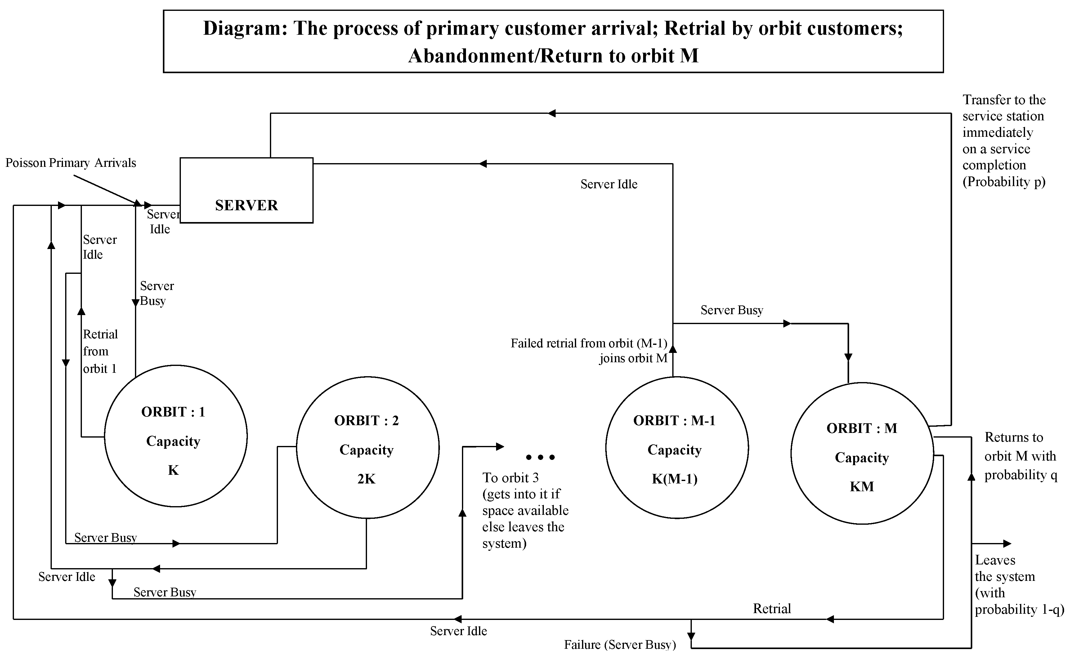
Figure 2.
Effect of p on .
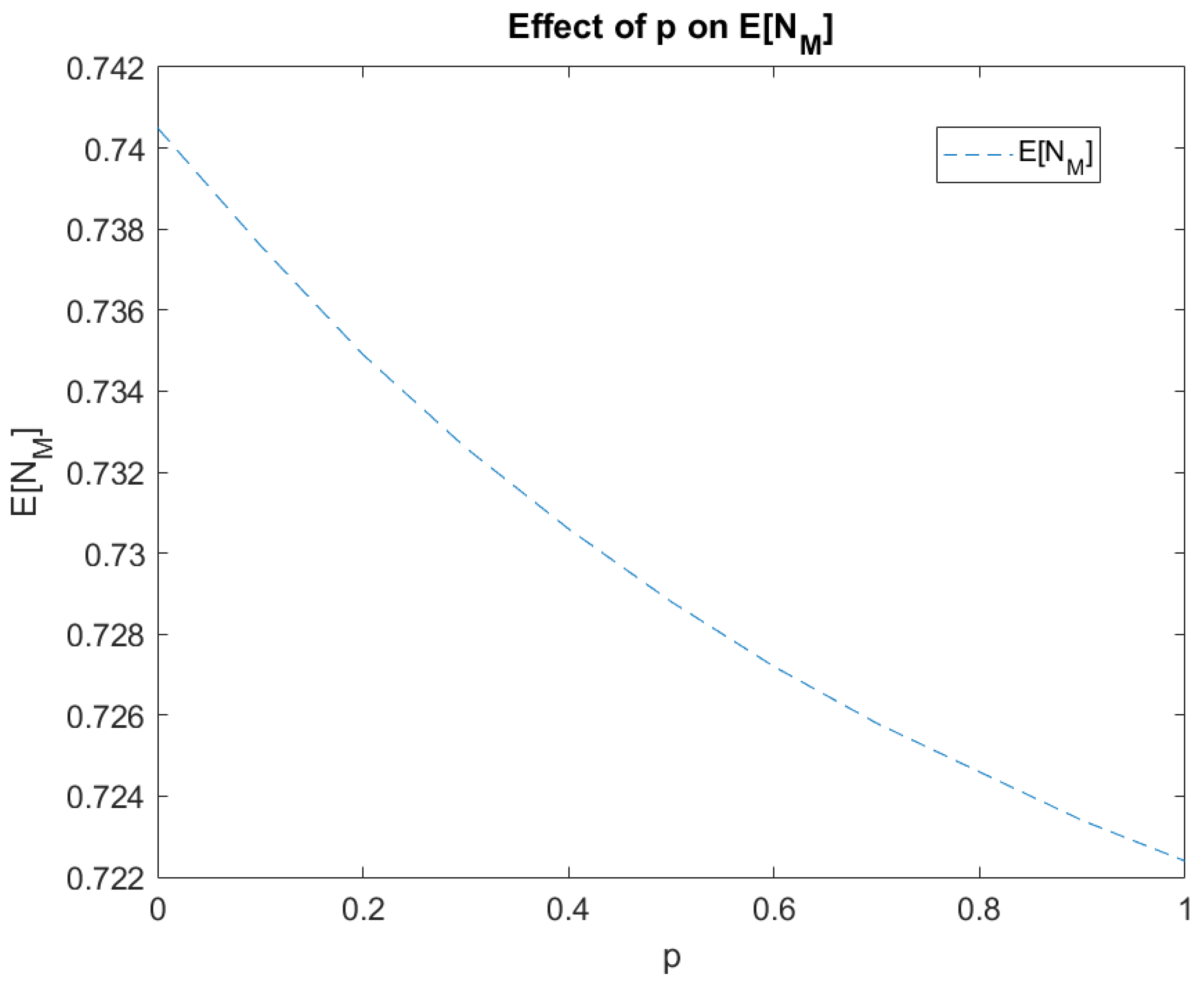
Figure 3.
Effect of p on number of customers in orbit-1.
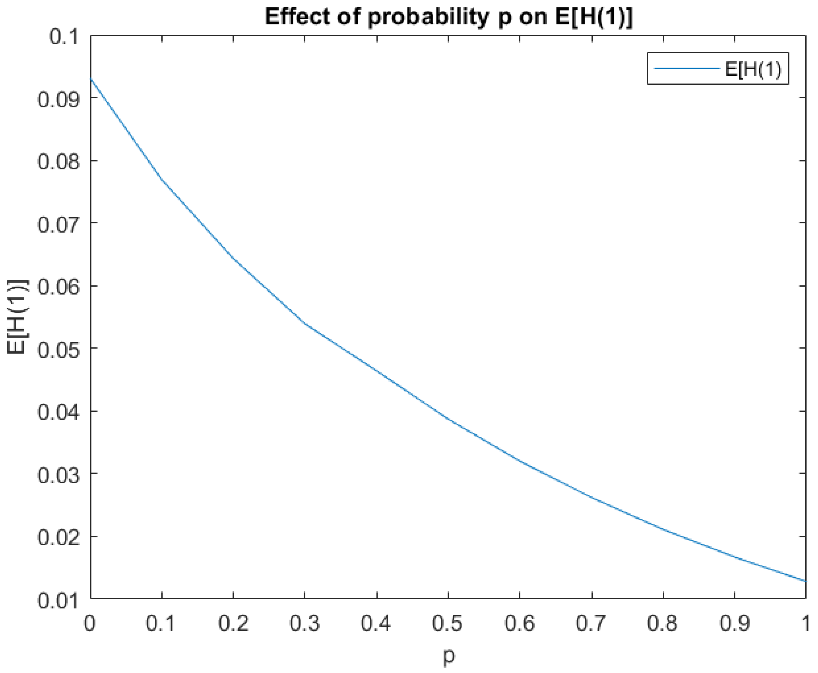
Figure 4.
Effect of p on .
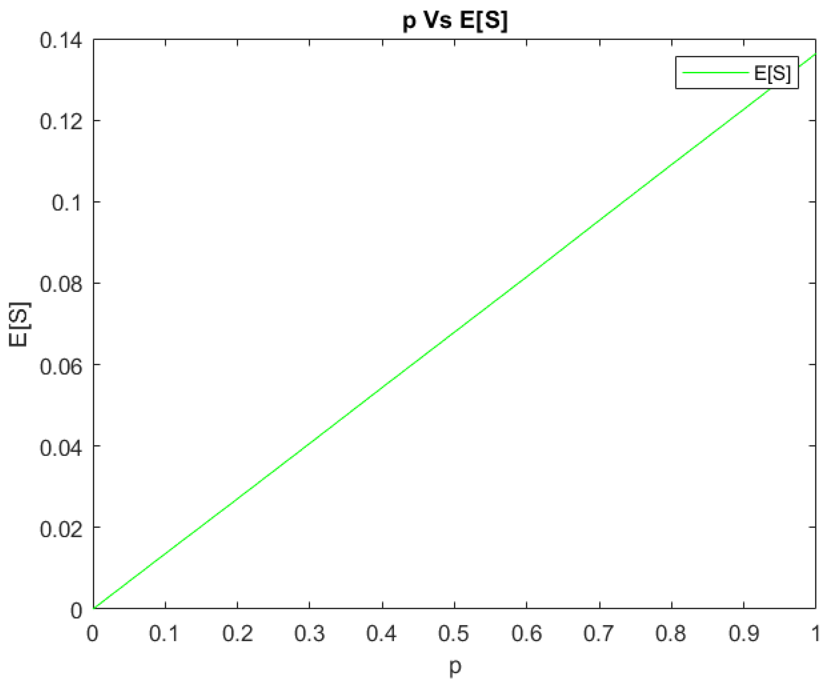
Figure 5.
Effect of p on .
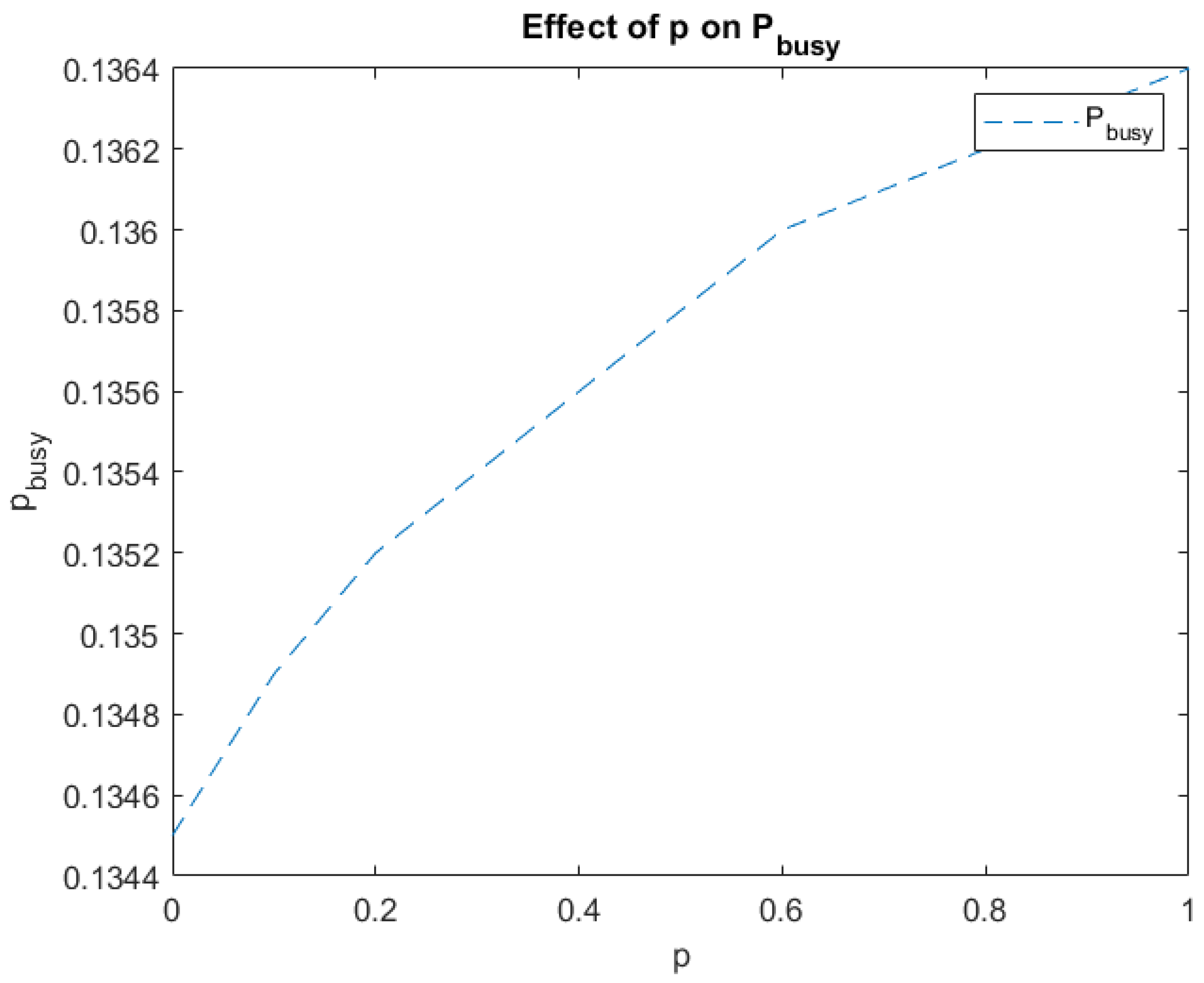
Figure 6.
Effect of p on .
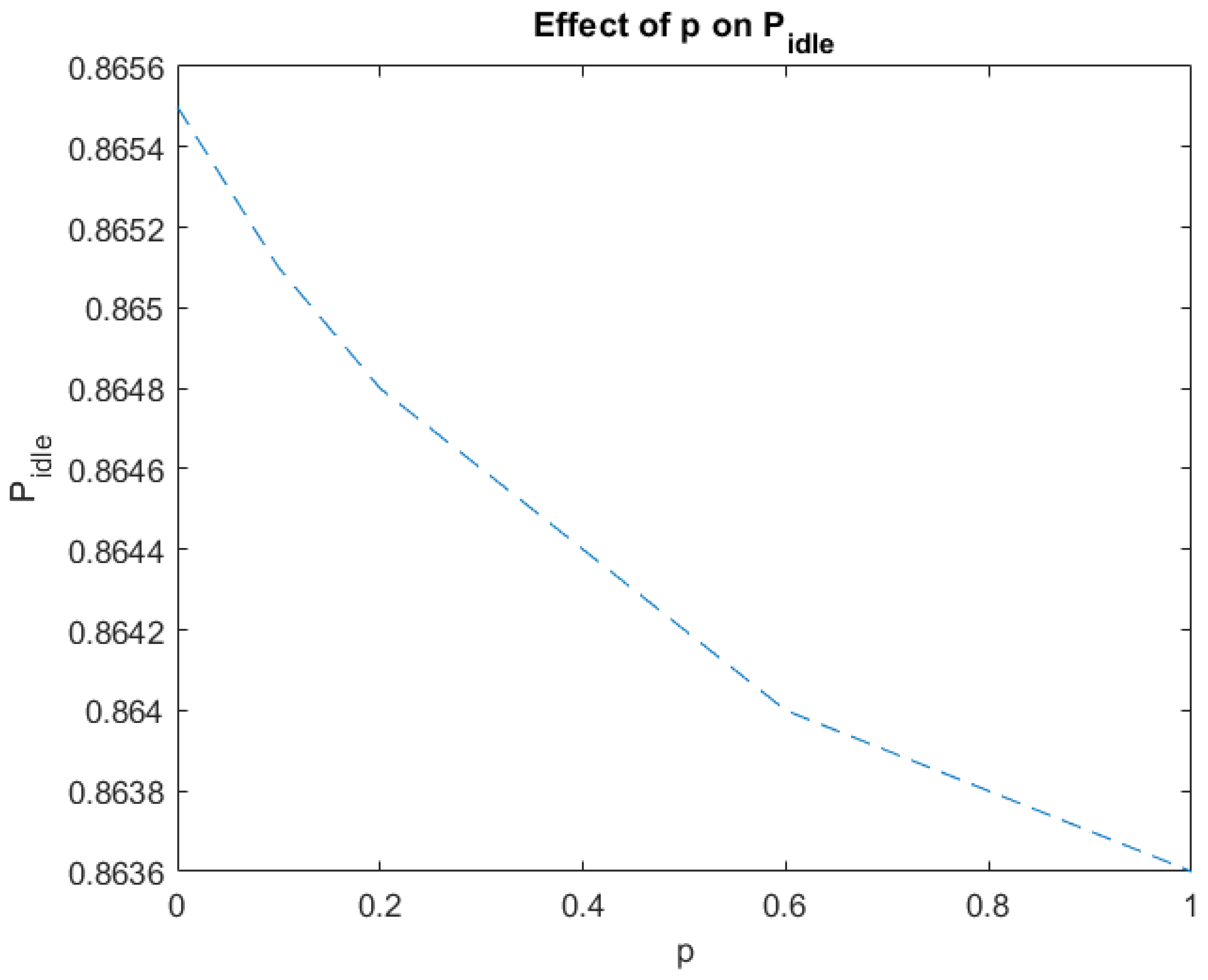

Table 1.
Rate of Transitions.
| From | To | Description | Transition Rate |
|---|---|---|---|
| arrival of | |||
| a primary customer | |||
| to an idle server | |||
| entry of | |||
| a customer to | |||
| the orbit-1 | |||
| successful retrial | |||
| from the | |||
| orbit-r | |||
| entry in to orbit-(r+1) | |||
| from the orbit-r, | |||
| successful search from orbit-M | |||
| unsuccessful search from orbit-M if | |||
| customers leave the system from orbit-M if | |||
| customers | |||
| leave the system | |||
| from orbit-r if | |||
| customers return to | |||
| orbit-M if | |||
| from orbit-M if |
Table 2.
Effect of Search probability p on System Performance measures.
| p | |||||
|---|---|---|---|---|---|
| 0 | 0.7405 | 0.0931 | 0 | 0.1345 | 0.8655 |
| 0.1 | 0.7376 | 0.0769 | 0.0136 | 0.1349 | 0.8651 |
| 0.2 | 0.7349 | 0.0643 | 0.0271 | 0.1352 | 0.8648 |
| 0.3 | 0.7326 | 0.0539 | 0.0407 | 0.1354 | 0.8646 |
| 0.4 | 0.7306 | 0.0464 | 0.0544 | 0.1356 | 0.8644 |
| 0.5 | 0.7288 | 0.0387 | 0.0680 | 0.1358 | 0.8642 |
| 0.6 | 0.7272 | 0.0320 | 0.0816 | 0.1360 | 0.8640 |
| 0.7 | 0.7258 | 0.0262 | 0.0954 | 0.1361 | 0.8639 |
| 0.8 | 0.7246 | 0.0211 | 0.1091 | 0.1362 | 0.8638 |
| 0.9 | 0.7234 | 0.0167 | 0.1227 | 0.1363 | 0.8637 |
| 1 | 0.7224 | 0.0128 | 0.1364 | 0.1364 | 0.8636 |
Disclaimer/Publisher’s Note: The statements, opinions and data contained in all publications are solely those of the individual author(s) and contributor(s) and not of MDPI and/or the editor(s). MDPI and/or the editor(s) disclaim responsibility for any injury to people or property resulting from any ideas, methods, instructions or products referred to in the content. |
© 2024 by the authors. Licensee MDPI, Basel, Switzerland. This article is an open access article distributed under the terms and conditions of the Creative Commons Attribution (CC BY) license (http://creativecommons.org/licenses/by/4.0/).
Copyright: This open access article is published under a Creative Commons CC BY 4.0 license, which permit the free download, distribution, and reuse, provided that the author and preprint are cited in any reuse.


