Preprint
Article

This version is not peer-reviewed.

Signal Preprocessing for Enhanced IoT Device Identification Using Support Vector Machine

A peer-reviewed article of this preprint also exists.

Submitted:

29 November 2024

Posted:

02 December 2024

You are already at the latest version

Abstract

Device identification based on radio frequency fingerprinting is widely used to improve the security of Internet of Things systems. However, noise and inconsistencies in raw radio frequency signals can reduce the accuracy of identification, classification, and authentication algorithms. This paper investigates how preprocessing methods affect the performance of a support vector machine classifier based on radio frequency fingerprinting. Four preprocessing methods are evaluated, each of which is applied to the raw radio frequency signals in an attempt to improve the consistency between signals emitted by the same Bluetooth device. Experiments conducted on a dataset of raw Bluetooth signals from sixteen smartphone radios, provided by Uzundurukan, show that selecting appropriate preprocessing methods can significantly improve the classification accuracy of a support vector machine classifier.

Keywords: 
;  ;  ;  ;  

1. Introduction

As the Internet of Things (IoT) rapidly expands across all sectors, including smart homes and industrial applications, connecting billions of devices, the need for robust and secure device identification becomes increasingly important. However, this growth also increases vulnerability to security threats, making reliable identification essential for securing IoT networks [1]. Limited security features and the wireless nature of many IoT networks make devices vulnerable to cyberattacks, including eavesdropping, spoofing, and unauthorized access, which can compromise entire networks  [2,3]. Traditional security methods, including passwords and encryption, are becoming less effective in IoT networks due to the limited resources of IoT devices and the scalability challenges posed by the rapid growth of connected devices [4]. Fortunately, device identification algorithms based on radio frequency fingerprinting (RFF) offer a promising solution to these challenges [5]. However, to be effective, RF fingerprints must conform to the principle of uniqueness [6], ensuring that each device, whether transmitting data or inactive, can be uniquely identified based on the intrinsic features of its RF signals. These features can be derived from the inherent variations introduced during the device manufacturing process. The key advantage of the RFF-based device identification algorithms is that they do not require any changes to the communication protocols on the RF devices and other IoT systems involved, nor do they require any additional hardware [6,7]. Thus, the RFF-based identification algorithms can provide a high level of security, making it difficult for attackers to replicate or spoof the distinctive RF fingerprint of a legitimate device. The effectiveness of these algorithms is inherently linked to the quality of the acquired RF signals [7]. Raw RF signals are often susceptible to noise, interference, and distortion, acquisition errors, or hardware imperfections. These factors can affect the performance of the identification algorithms that rely on RF fingerprints to accurately classify devices. As a result, signal preprocessing becomes an indispensable tool for improving the quality of the RF signals used in the identification process. Signal preprocessing methods are used to standardize the input data ensuring that it meets the specific requirements of the classifier. Choosing the right preprocessing method is crucial to accurate device identification [8].
RF fingerprinting is a useful technique for identifying IoT devices. For example, in 2019, Tu et al. [9] studied four types of RF fingerprint feature extraction algorithms based on statistical features. They used an SVM-based classifier and applied the robust principle component analysis (RPCA) to reduce its dimensionality. Also, in 2019, Nouichi et al. [10] proposed an approach to detect emitted wireless signals from IoT devices based on a software defined radio (SDR), considering that the cryptography-based authentication protocols are impractical for the IoT systems. On the other hand, in 2020, Aghnaiya et al. [11] investigated the identification of WiFi devices using RF device fingerprints. They demonstrated that intrinsic features of RF devices can be effectively used to detect and classify them. Also, in 2020, Lin et al. [12] proposed a method based on the detection of complex and nonlinear patterns arising in the interaction between different frequency components of RF signals to recognize wireless devices. Similarly, in 2020, Uzundurukan et al. [2] developed an RF fingerprinting system to identify Bluetooth devices. They demonstrated that their strategy was effective in distinguishing between different Bluetooth devices operating in a crowded IoT system. In 2022, Morge-Tollet et al. [13] highlighted the RF fingerprinting as a reliable option for the node authentication in IoT networks as a non-cryptographic method. They proposed an RF eigen-fingerprinting method based on singular value decomposition (SVD), which is inspired by face recognition studies based on the Ljung-Box test, a statistical authentication approach. Also, in 2022, Chen et al. [14] proposed a method based on on convolutional neural networks (CNN), combinatorial randomness, and on-chip time-varying RF fingerprints, which have been lightweight-implemented for Bluetooth Low-Energy (BLE) systems to achieve a fast inference of unique features in the IoT environments. In 2024, Peng et al. [15] proposed a method based on the wavelet coefficient graph and differential spectrum to identify signal inconsistencies in Long Term Evolution (LTE) systems.
In this context, it is also worth reviewing the survey prepared in 2023 by Xie et al. [16], where they considered the following signal preprocessing stages in the identification process: i) RF fingerprint extraction, ii) further processing, and iii) RF fingerprint identification. They also summarized the carrier frequency offset estimation, denoising, and channel cancellation. Finally, they highlighted the major challenges of the RF fingerprint identification and some future research trends.
In any case, the RFF methods face significant implementation and security challenges when intended for IoT scenarios. Techniques like time synchronization and frequency correction require significant computational resources, which can slow down processing, especially for large datasets or in real-time applications [15]. Similarly, feature extraction methods are resource-intensive, requiring significant memory and processing power, which can make them impractical for resource-constrained IoT devices [12]. The sequential nature of preprocessing can introduce latency, affecting the system’s ability to perform real-time identification in dynamic environments [14]. In addition, early stages of preprocessing are often sensitive to noise, leading to potential errors in pattern recognition and feature extraction [12]. While dimensionality reduction optimizes the feature set, it may inadvertently discard important details, affecting classification accuracy [14]. Implementing and fine-tuning these preprocessing steps also requires specialized expertise, and even small errors in configuration can affect system performance. Furthermore, the effectiveness of preprocessing is highly dependent on the quality of the signal acquisition hardware; inconsistent or low-quality hardware can degrade the entire process, reducing the reliability of RFF systems [15].
On the other hand, the supervised learning algorithms have been widely used for RFF-based classification systems. Support vector machine (SVM), random forest, and neural network (NN) are strategies that have demonstrated significant potential for detecting the intrinsic RF signals of IoT devices. For example, in 2018, Jafari et al. [17] proposed a wireless device identification platform based on RF device features to improve the security of IoT networks by using deep learning techniques. They used deep, convolutional, and recurrent NN to identify the wireless devices, including whether the devices are from the same manufacturer. On the other hand, in 2019, Yu et al. [18] used the RFF approach in an SVM-based classifier to identify ZigBee devices, achieving a suitable level of classification accuracy. Also, in 2019, Ali et al. [19] compared the performance of machine learning models and found that SVM-based identification algorithms provide an optimal balance between computational efficiency and classification performance for resource-constrained environments, such as those found in IoT systems. In 2022, Huang et al. [20] proposed a classification RFF-based method to improve the effectiveness of a classifier based on ensemble learning and a CNN. Also, in 2022, Yang et al. [21] proposed a CNN&RFF-based model to implement a lightweight classifier. It is also worth reviewing the survey prepared in 2022 by Jagannath et al. [22] presented a survey of RF fingerprinting approaches considering from a traditional view to the latest deep learning-based algorithms.
To address these challenges, this paper contributes by evaluating four signal preprocessing methods based on the normalization, mean, maximum, and minimum of the raw signals to improve data consistency and enhance classification accuracy. These methods were selected because they address common issues in raw RF signals, such as variability in signal strength and noise, which can negatively affect the performance of classification algorithms. By scaling the signal peaks, these preprocessing methods aim to standardize the input data, ensuring that key signal features are more effectively captured and utilized by the classifier. An SVM classifier, known for its effectiveness in binary and multi-class tasks, is used to assess the impact of these preprocessing methods, building on the work of [2]. The findings show that RFF requires careful extraction of a device’s unique signal characteristics to effectively distinguish between classes.
The paper is divided into five sections. Section 2 provides a comprehensive overview of the dataset, which consists of Bluetooth signals from multiple devices. It provides the definition and characteristics of these signals, and it details the preprocessing methods. In addition, this section describes the configuration of the SVM classifier, including the selection of the kernel, and the experimental setup for training and testing. 
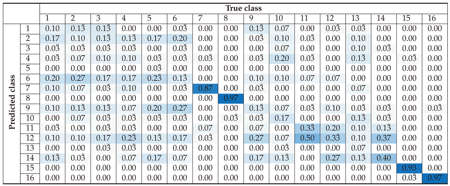
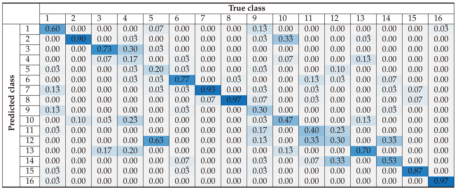
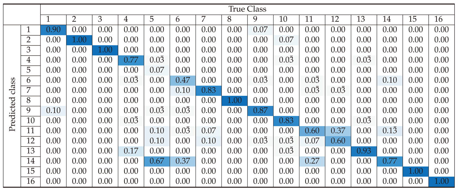
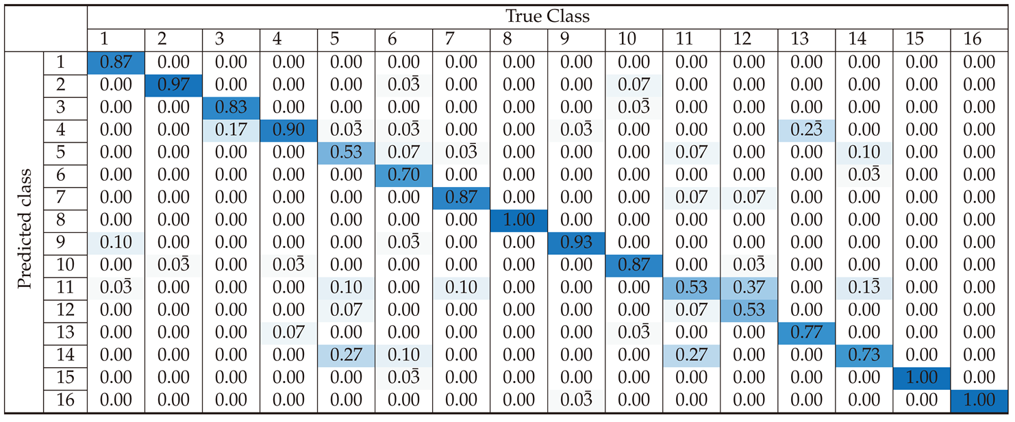
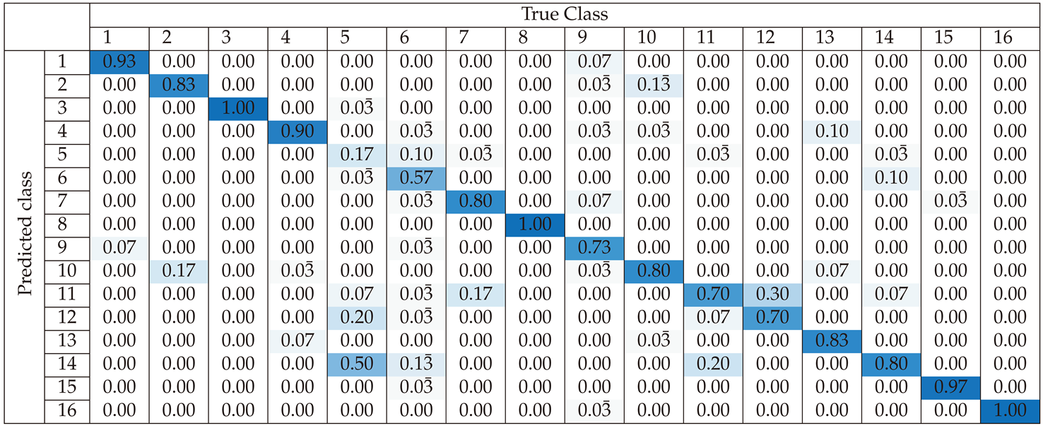
Section 3 presents the classification performance for each preprocessing approach, using confusion matrices and accuracy metrics to evaluate the effectiveness of the SVM-based classifier. This section demonstrates how different preprocessing methods influence classification accuracy across various device classes. Section 4 offers an in-depth analysis of the results, highlighting the strengths and weaknesses of each preprocessing method. It examines the causes of misclassifications and discusses the balance between improving accuracy and maintaining computational efficiency. This section also identifies potential areas for optimization, such as improving the model robustness to noise and its ability to generalize across different datasets. Lastly, Section 5 summarizes the key findings, emphasizing the importance of preprocessing in enhancing the effectiveness of RFF-based device identification. It discusses the broader implications for IoT security and proposes future research directions, including advanced feature extraction, real-world validations, and the exploration of alternative machine learning models to further enhance classification performance.

2. Materials and Methods

2.1. Dataset Description

The dataset used in this work was extracted from the RF signal dataset created by Uzundurukan et al. [3]. They captured RF signals from 27 smartphones, representing six different manufacturers, and it serves as a comprehensive resource for RFF. For each Bluetooth, they captured 150 RF signals, for a total of 12,900 signal recordings. They collected the RF signals under controlled laboratory conditions to minimize external interference and to ensure high data quality and consistency. In the Uzundurukan dataset includes RF signals recorded at 5 Gsps, 10 Gsps, and 20 Gsps using a Tektronix TDS7404 oscilloscope. In addition, lower-frequency signals were acquired at 250 Msps using a modular RF front-end system connected to the oscilloscope. For this work, 16 smartphone radios were selected and paired as twins, representing eight different brands. Each smartphone was assigned to a specific class, where devices within the same pair (or twin) belong to the same model but are treated as different classes. For instance, as shown in Table 1, Class 1 corresponds to "iPhone 5 - 1," while Class 2 corresponds to its twin, "iPhone 5 - 2." Similarly, this pattern continues for other models, ensuring that each twin device is categorized into its unique class.
Understanding the distinctions between these classes is critical for evaluating RFF performance, as subtle variations between twin devices test the robustness of the classification algorithm. These class distinctions are further explored in the next section, where the definition and characteristics of raw Bluetooth signals are discussed in detail. This provides the foundation for analyzing how these signals can be used to uniquely identify devices within and across classes.

2.2. Definition and Characteristics of Raw Bluetooth Signals

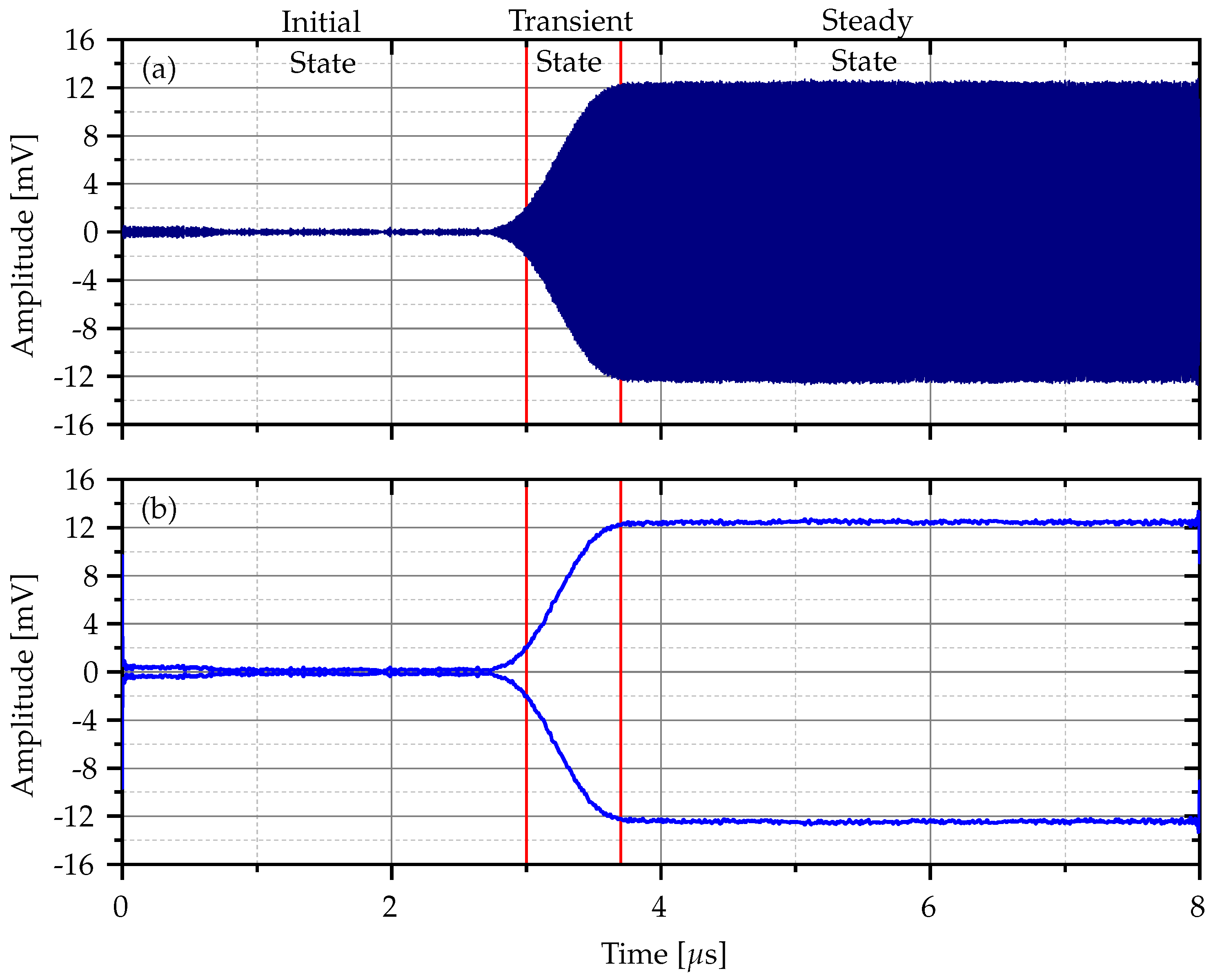
Each Bluetooth signal carries intrinsic features that form the basis of RFF, which allows devices to be identified based on their unique characteristics. As the signals transition through three distinct states, these features become more apparent. Figure 1a shows how the complete Bluetooth signal as detected by the receiver, while Figure 1b highlights the envelope of the signal, making it easier to observe the transitions between these states.
The first state, known as the initial state, captures only the internal noise generated by the Bluetooth receiver. At this stage, the transmitter has not yet started sending signals, and the noise from the receiver serves as a baseline for further analysis. Once the transmitter is activated, the signal enters the transient state. During this phase, the receiver begins to detect the intrinsic noise from the transmitter in addition to its own noise. This state reflects the transition as the Bluetooth transmitter ramps up, providing valuable insight into the device’s unique signal behavior. Finally, the signal reaches the steady state, where both the intrinsic noise of the transmitter and the receiver are combined. This phase represents the full interaction between the two devices and captures the overall noise profile of the communication system.
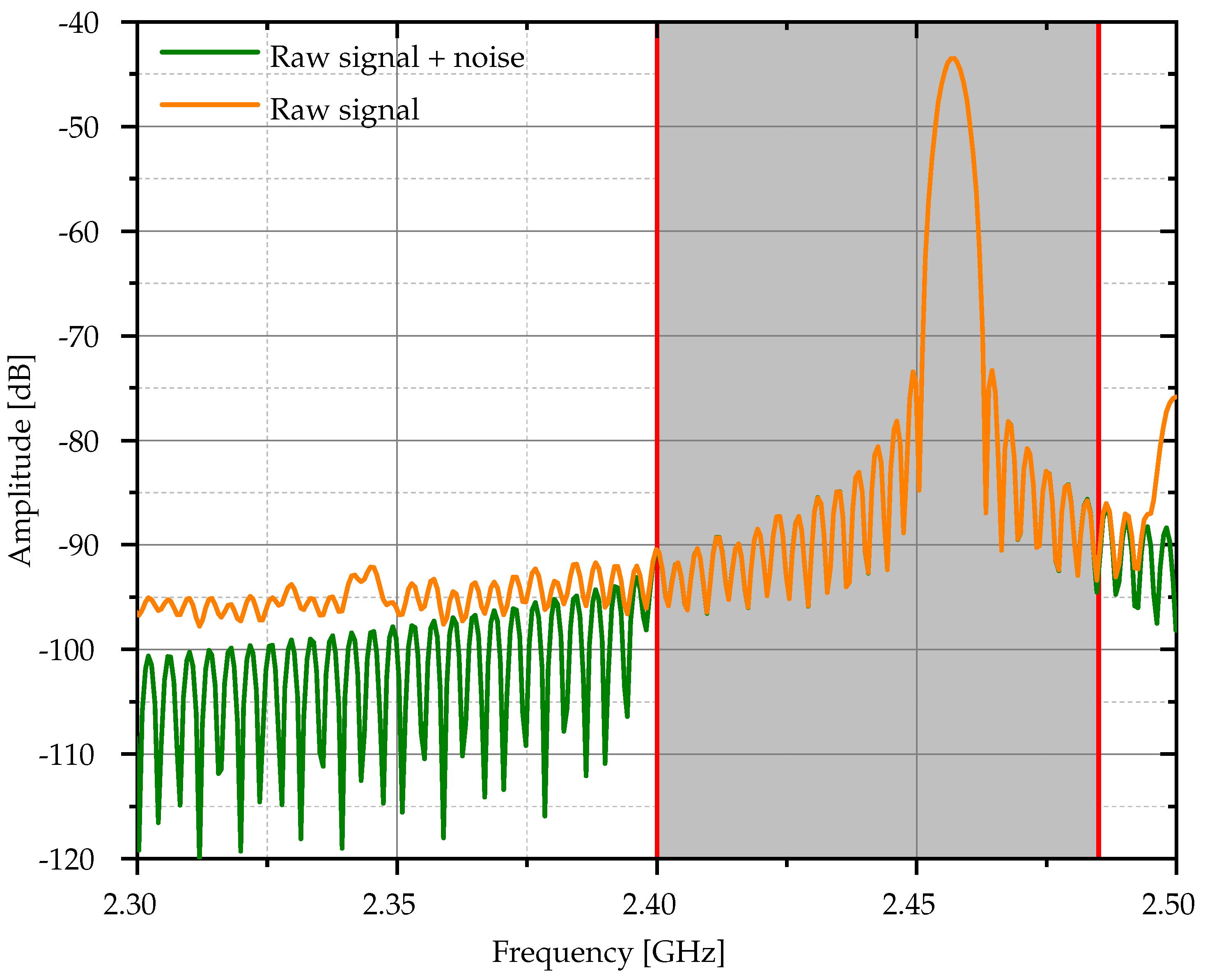
On the other hand, Figure 2 illustrates the frequency spectrum of a Bluetooth signal, highlighting the presence of unwanted frequencies combined with noise, which includes the environmental electromagnetic interference and the system noise. This feature highlights the importance of implementing a bandpass filter to improve the signal fidelity. The bandpass filter extracts the signal in the range from 2.40 GHz to 2.48 GHz. The shaded gray area in Figure 2 highlights the effect of the bandpass filter. This process ensures that the raw signal provided to subsequent preprocessing methods is cleaner, allowing for more accurate analysis and classification in RFF tasks. Therefore, the raw Bluetooth signal represents the unprocessed transmission captured directly from the target device. This signal contains intrinsic features derived from the device hardware, specifically from the transmitter. These features make the raw signal a rich source of information that can be used as a radio frequency fingerprint because they reflect unique device-specific attributes.
However, the raw signal also has a wide range of frequencies, often containing unwanted frequencies and noise that can obscure the critical features needed for accurate classification. Without preprocessing, such as filtering or scaling, the quality of the raw signal can be degraded, resulting in reduced performance of machine learning models. Therefore, preprocessing methods such as bandpass filtering are essential to isolate the primary signal components and ensure that the raw signal is suitable for further analysis.

2.3. Preprocessing Methods

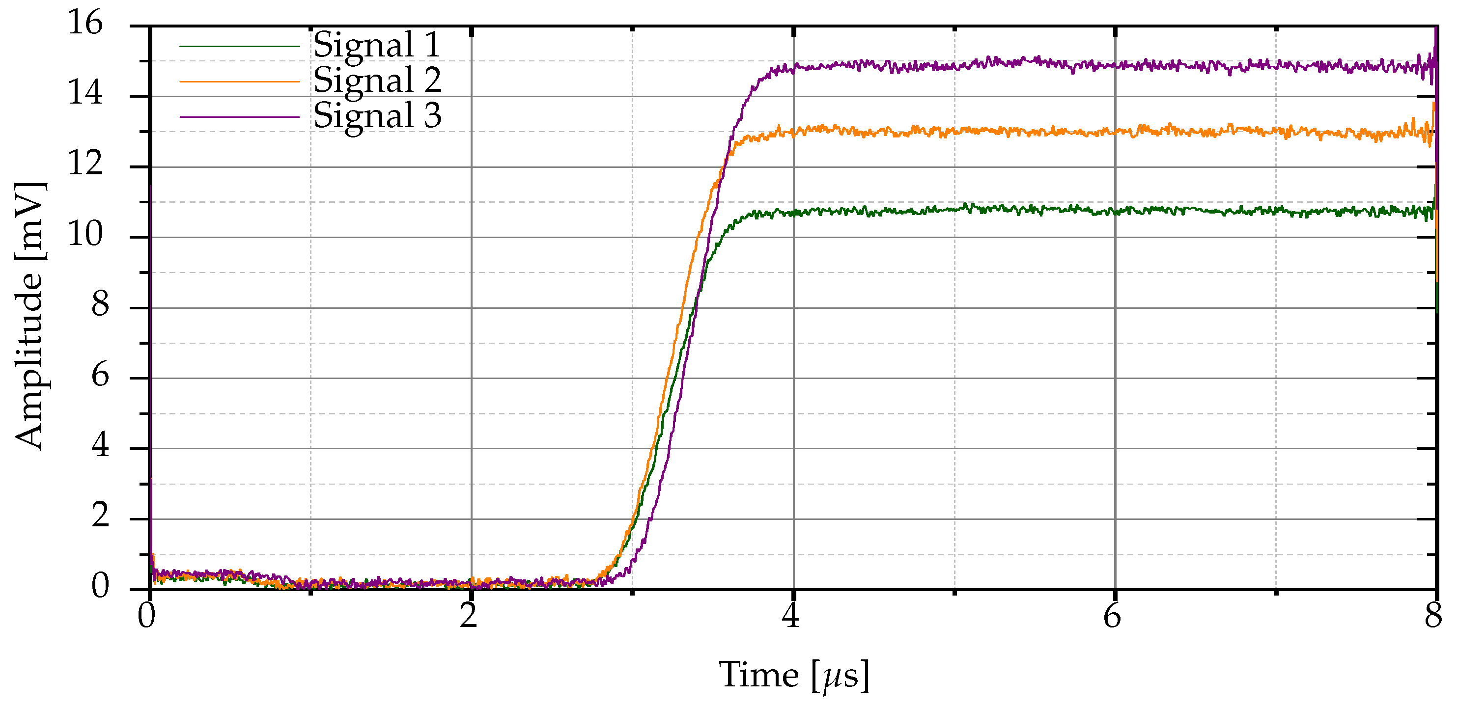
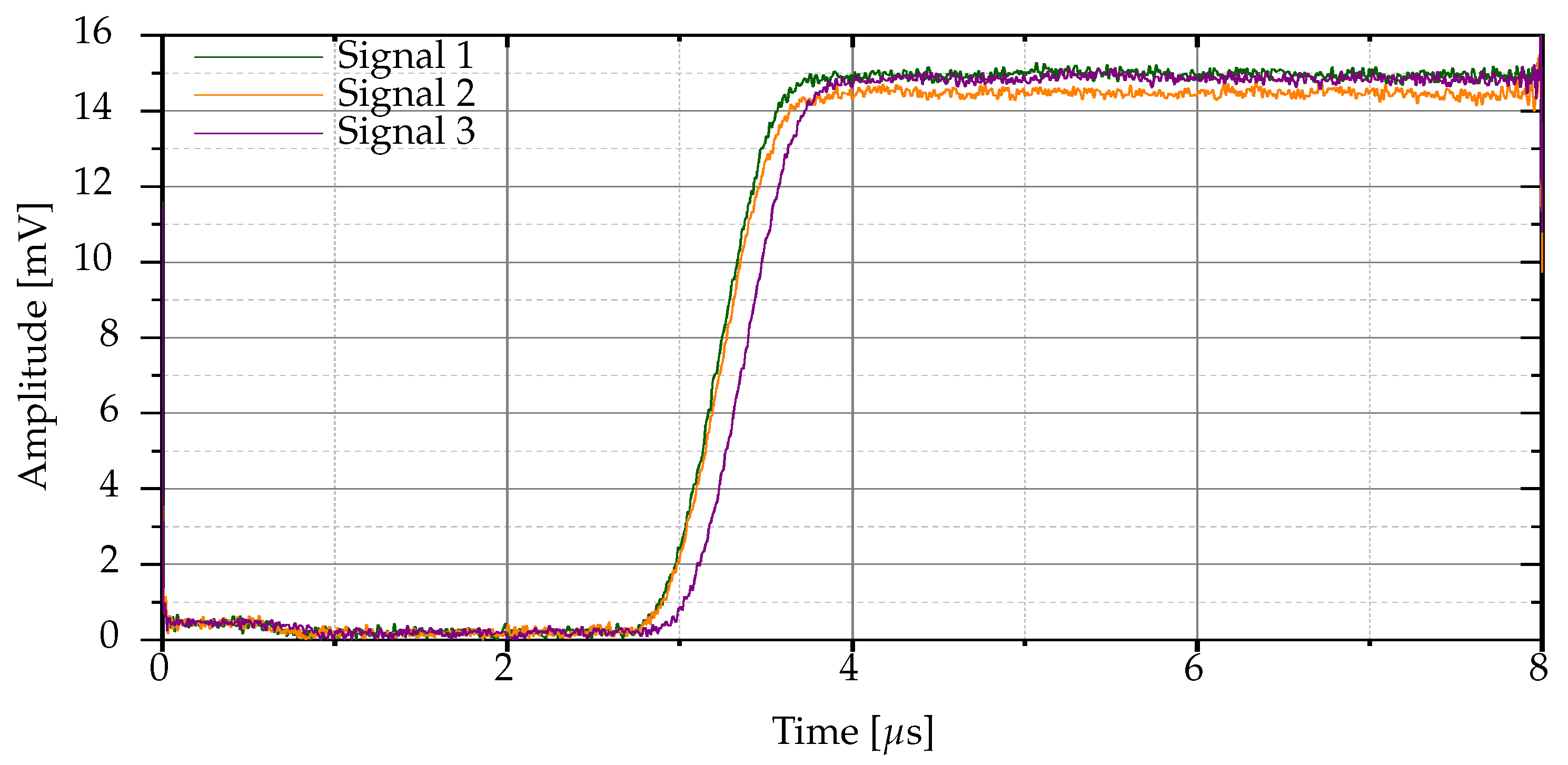
The preprocessing methods must standardize the signals used in an analysis to ensure that the signal features can be interpreted by the classifier. Figure 3 shows the envelopes of the three radio frequency signals acquired from the same Bluetooth device, which have some differences.
Therefore, in this study, four preprocessing methods are defined to adjust the amplitude of the raw Bluetooth signals. These methods are defined as follows and are designed to improve data consistency and improve the classification accuracy by emphasizing key features of the raw Bluetooth signals and improving the performance of a classification algorithm.
Definition 1
(Scaled signals). The signal p i ( t ) , given in Eq. 1, is the scaled variant of the Bluetooth signal s i ( t ) , assuming that α / A i p e a k is the scaling factor, A i p e a k = m a x | s i ( t ) | represents the maximum magnitude reached by s i ( t ) , and α is a dynamic term for adjusting the scaling factor that depends on the selected preprocessing method.
p i ( t ) = α A i peak · s i ( t ) ,
where i = 1, 2, 3, ... N.
Definition 1 ensures that the raw Bluetooth signals are dynamically adjusted based on A i p e a k and α , preserving their time-varying features and avoiding the significant differences in amplitude of a variety of Bluetooth signals produced by the same device.
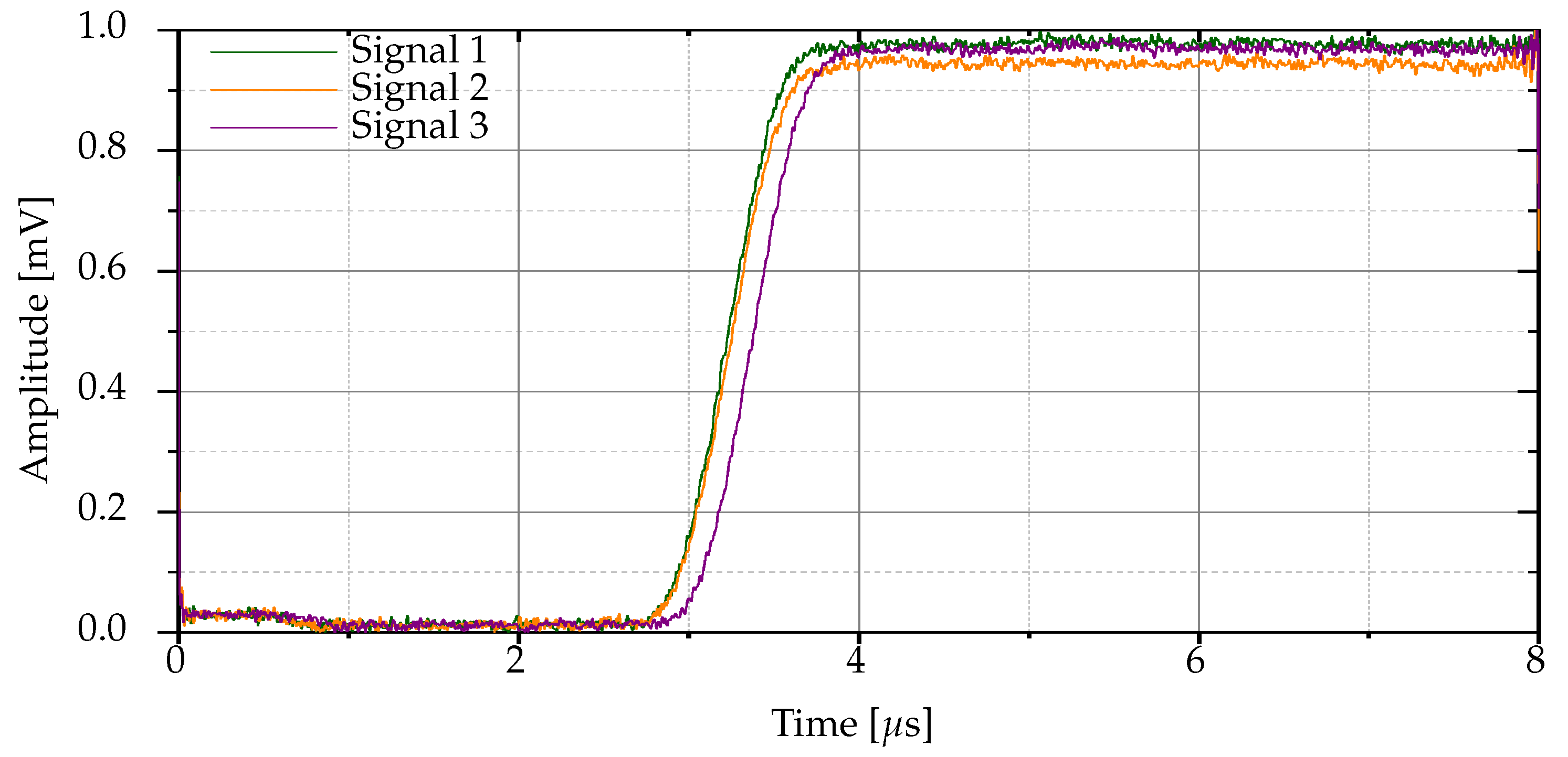
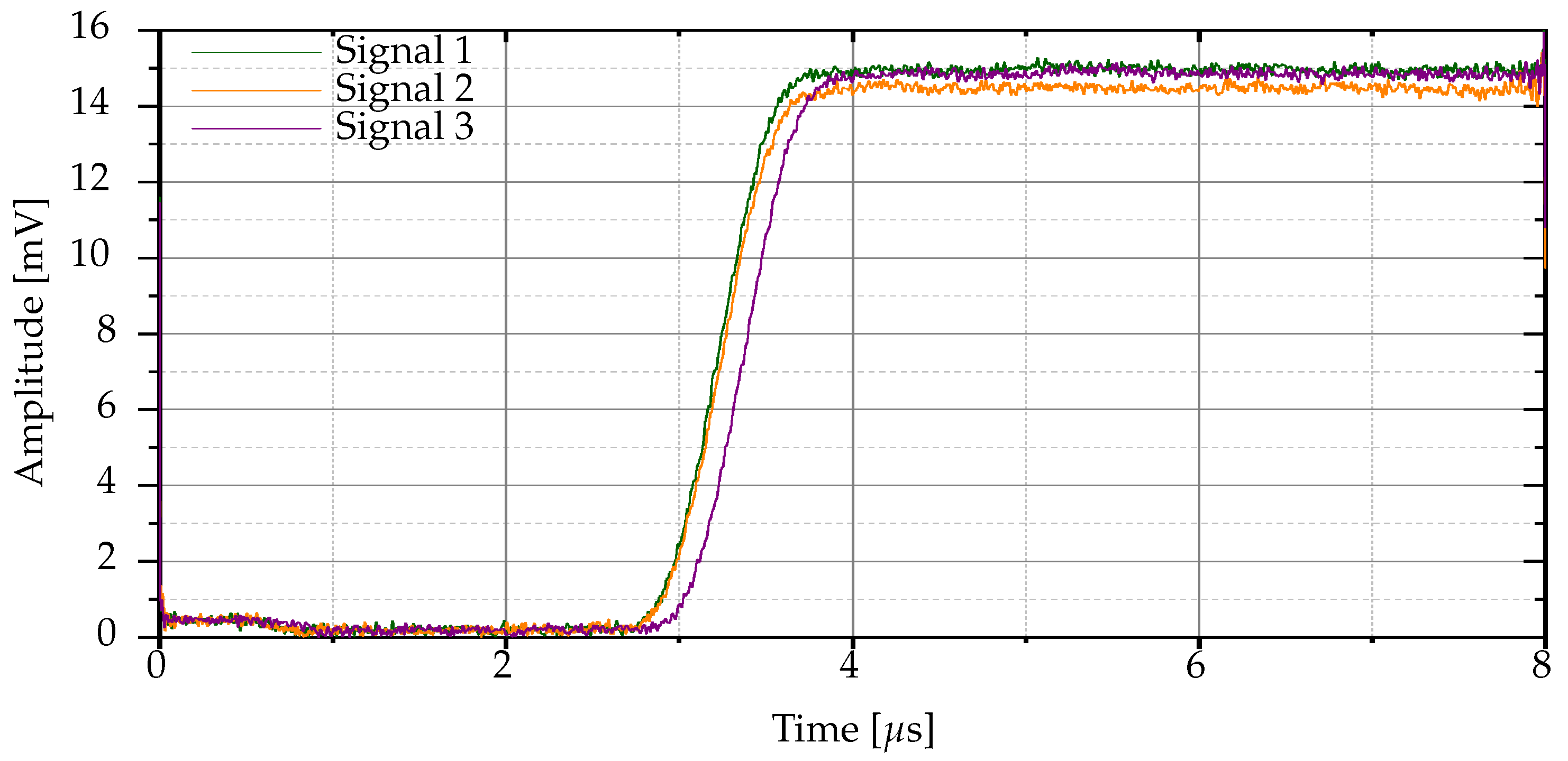
Definition 2
(Normalized raw signals). p i ( t ) is the normalized variant of s i ( t ) when α = 1 , meaning that s i ( t ) is scaled by its maximum value, without any other scaling adjustment.
The envelopes of the normalized variants computed for the Bluetooth signals in Figure 3 are shown in Figure 4.
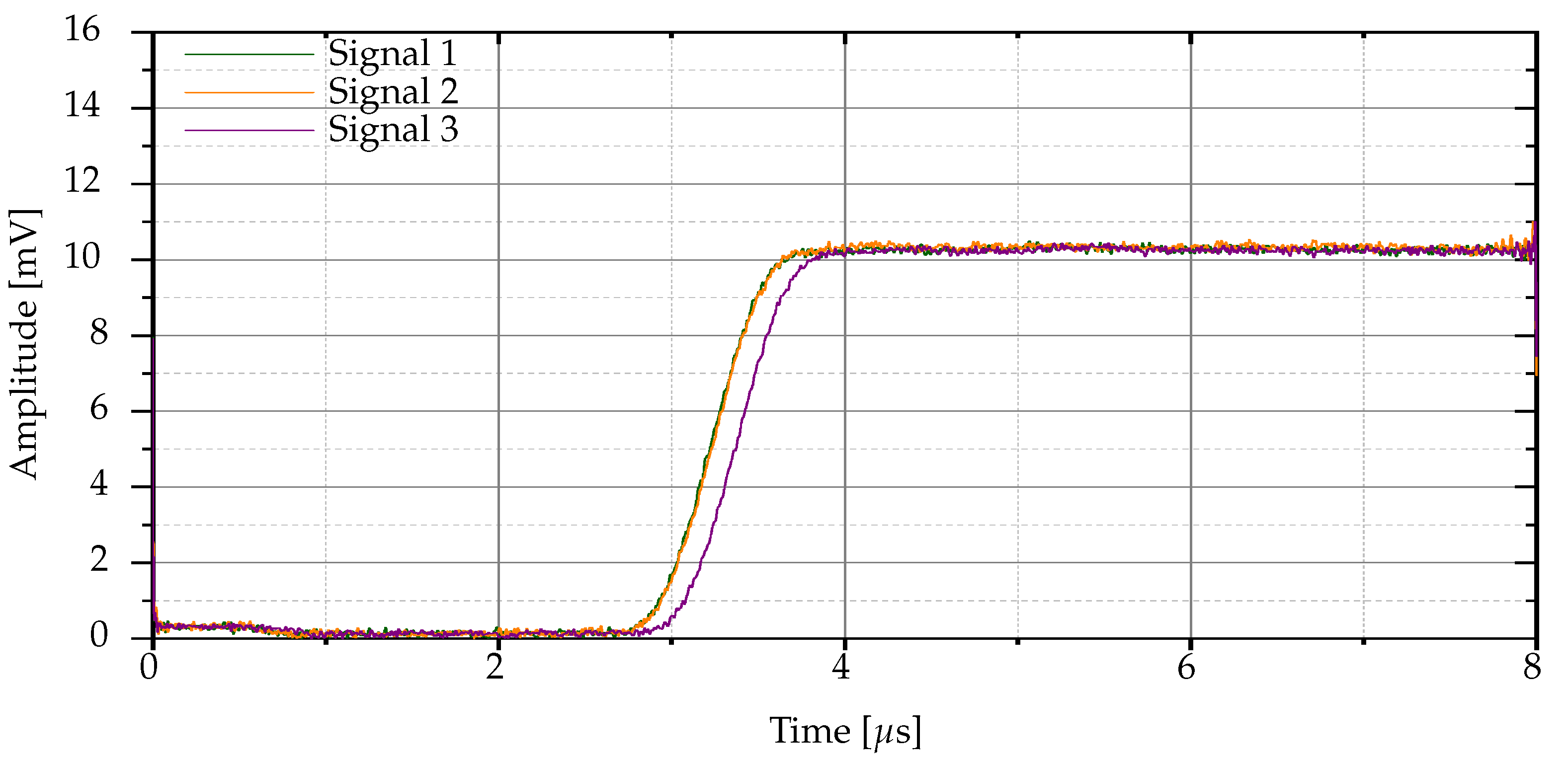
Definition 3
(Mean-normalized raw signals). p i ( t ) is the mean-normalized variant of s i ( t ) when α is computed using Eq. 2 and N Bluetooth signals from the same Bluetooth device are considered.
α = 1 N i = 1 N A i p e a k .
It should be noted that this approach reduces the signal variability by applying a global scaling factor. Figure 5 illustrates the envelopes of the mean-normalized raw signals for the three Bluetooth signals of Figure 2. Typically, N = 150 .
Definition 4
(Max-normalized raw signals). p i ( t ) is the max-normalized variant of s i ( t ) when α is computed using Eq. 3 and N Bluetooth signals from the same Bluetooth device are considered.
α = max A i p e a k .
This approach uses the global maximum in the set of Bluetooth signals from same device. Figure 6 illustrates the envelopes of the max-normalized raw signals for the three Bluetooth signals of Figure 2.
Definition 5
(Min-normalized raw signals). p i ( t ) is the min-normalized variant of s i ( t ) when α is computed using Eq. 4 and N Bluetooth signals from the same Bluetooth device are considered.
α = min A i p e a k .
This approach minimizes the influence of high peaks in the set of Bluetooth signals from the same device, emphasizing lower signal components. Figure 7 illustrates the envelopes of the min-normalized raw signals for the three Bluetooth signals of Figure 2.

2.4. Classifier Description and Experimental Setup

The SVM classifier was parameterized in accordance with the methodology outlined in [2], utilizing a quadratic polynomial kernel to effectively handle complex, non-linear relationships in Bluetooth signal data. The data split was conducted randomly to ensure robust and unbiased evaluation, while feature extraction focused on higher-order statistics (HOS) derived from transient Bluetooth signals, providing a rich set of attributes for classification.
The implementation was performed using MATLAB, facilitating efficient data processing and experimentation. The computational setup for this study included a device with the following specifications: AMD Ryzen 5 2500U with Radeon Vega Mobile Graphics at 2.00 GHz, 32 GB of RAM (30.9 GB usable), and a 64-bit operating system. This hardware configuration ensured smooth execution of the computationally intensive tasks associated with SVM training and testing. The results highlight the classifier’s potential as a powerful tool for RFFs, particularly when optimized for transient signal characteristics.
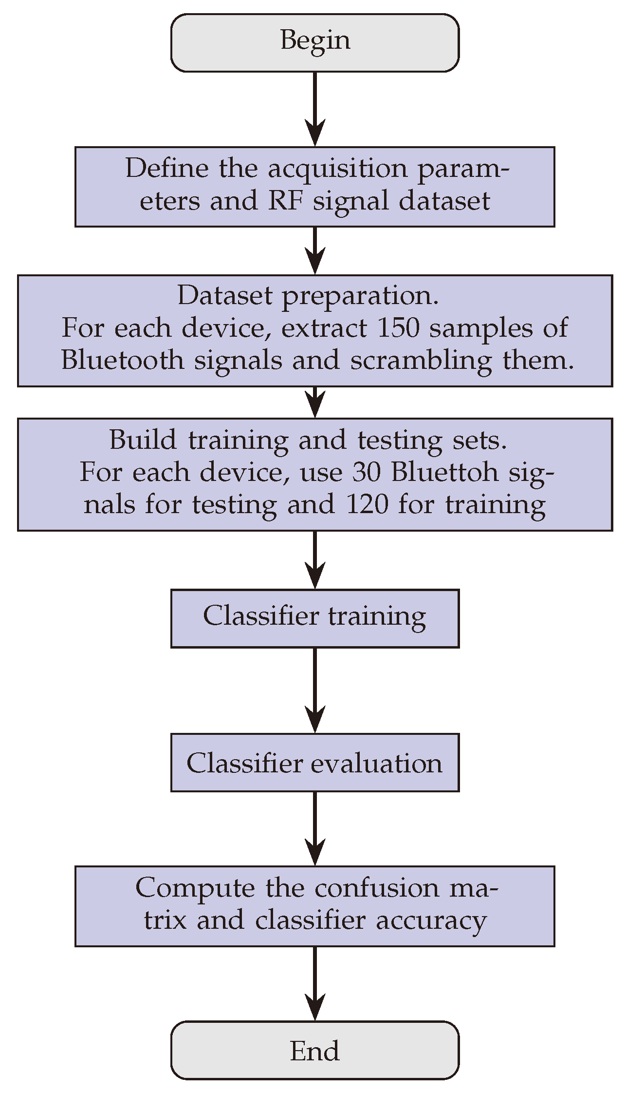
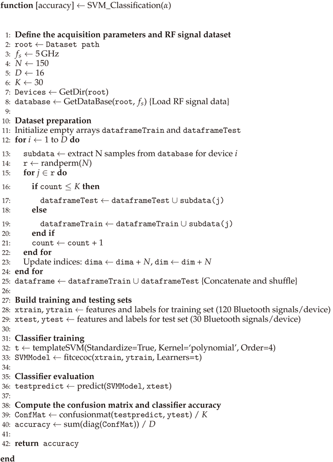
The SVM-based classifier procedure is illustrated step-by-step in the Algorithm 1. It begins with loading the parameters and the RF dataset, which includes preparing the data for analysis. The dataset preparation involves creating separate storage for training and testing data, followed by iterating through each device to extract 150 signal samples. For each device, 30 samples are reserved for testing while the remaining 120 are used for training.
Afterward, the training and test sets are concatenated and shuffled to ensure a randomized distribution of data. The data is then split into features and labels for the training and test sets, using xtrain and ytrain for the training data and xtest and ytest for testing. The algorithm proceeds by training an SVM model using a polynomial kernel with an order of 4, ensuring that the data is standardized to improve training consistency. Once the model is trained, it is evaluated on the test set, with predictions being generated for the test samples. To assess the model’s performance, a confusion matrix is computed, and the accuracy is calculated by comparing the predicted labels to the true labels. The procedure concludes by outputting the overall classification accuracy, which provides insight into the model’s effectiveness. The flowchart in Figure 8 captures the entire process, ensuring a comprehensive overview of the algorithm’s workflow from data loading to final evaluation, this process aligns with the algorithm detailed in Algorithm 1.
Algorithm 1 SVM-based classifier
Preprints 141374 i006

3. Results

This section presents the evaluation of the performance of an SVM-based classifier when different preprocessing methods are applied to RF signals extracted from the dataset B developed by Uzundurukan et a. [2]. The evaluation focuses on assessing the effectiveness of the classifier using two different performance metrics. The first metric, referred to as the diagnostic accuracy, is defined as the mean value of the diagonal elements of the confusion matrix. This metric quantifies the overall effectiveness of the SVM-based classifier by encompassing all classes and representing the percentage of correct classifications over the entire dataset when the evaluator has previously confirmed which is the Bluetooth device of the RF signal being analyzed. It provides a comprehensive measure of the overall performance of the SVM-based classifier in accurately identifying devices. In contrast, the second metric, effective accuracy, delves into the mean effectiveness of the SVM-based classifier considering the class assignment criterion determined by the maximum values in each column of the confusion matrix. Since each column in the confusion matrix sums to one, the SVM-based classifier assigns each instance to the class based on the maximum value in its respective column. To compute this metric, the frequency with which the classifier correctly assigns instances to their actual classes is determined by identifying the maximum values in each column and verifying their correspondence to the correct class. Each correct assignment is equally weighted in the final effectiveness of the classifier, reflecting the total number of hits divided by the number of classes.

3.1. SVM-Based Classifier with Raw Signals

The performance of the SVM-based classifier on raw Bluetooth signals was evaluated using the confusion matrix shown in Table 2. Some classes are effectively classified due to the presence of well-defined maximum values on the diagonal of the matrix. For example, classes 7, 8, 12, 14, 15, and 16 have maximum values of 0.87, 0.97, 0.33, 0.40, 0.93, and 0.97, respectively, indicating that the classifier was able to detect them. However, this is not the case for other classes, which leads to confusion. Note that in several columns, the maximum value is not on the diagonal. To illustrate this condition, the highest value for class 6 is in row 9, indicating classification errors. A similar phenomenon is observed for classes 1, 2, and 3, where the values are scattered across multiple rows, making the accurate assignment difficult. The uneven distribution of values also affects the accuracy of the model, which is relatively low, with a diagnostic accuracy of 35.42% and an effective accuracy of 37.5%. This is due to the fact that the decision criterion favors classes with high values in several columns, even though they do not correspond to the actual class.

3.2. SVM-Based Classifier with Normalized Raw Signals

The confusion matrix in Table 3 illustrates the performance of the SVM-based classifier when applied to normalized raw Bluetooth signals. This is confirmed by both accuracy metrics, which reach 61.25% for diagnostic accuracy and 81.23% for effective accuracy and indicating superior performance compared to previous scenarios. The classes that were correctly classified had clear maximum values on the diagonal of the matrix. For instance, class 7 had a value of 0.93, while class 8 reached 0.97. Similarly, classes 15 and 16 had maximum diagonal values of 0.87 and 0.97, respectively, confirming their status as well-resolved cases. Nevertheless, some confusion remains in certain classes, where the maximum values were not located on the diagonal. For instance, class 4 had a maximum of 0.30 in the row corresponding to class 3, indicating a notable degree of confusion between these two categories. Similarly, although class 9 had a maximum value of 0.30 on its own row, it also had notable values on other rows, such as 0.13, indicating some dispersion in the predictions. In contrast, Class 10 reached a maximum of 0.47 on the diagonal, but also had a notable value of 0.33 on the row corresponding to Class 2, indicating of significant confusion. Overall, the distribution of values in the matrix is is more uniform as a result of the normalization process. However, some classes still showed difficulty in correctly assigning predictions. This behavior is particularly evident in classes 4, 5, and 12, where the scatter of values affects the accuracy of the model.

3.3. SVM-Based Classifier with Mean-Normalized Raw Signals

The confusion matrix in Table 4 shows the performance of the SVM-based classifier when using mean raw signals. The results were 78.96% for the diagnostic accuracy and 93.75% for the effective accuracy. This is evidence of significant improvement in the signal classification. In this case, the confusion matrix showed a remarkable degree of consistency along the main diagonal, with values approaching 1 for a significant number of classes. For example, classes 2 and 3 showed optimal performance, with values of 1.00 on the diagonal, indicating that these categories were classified with higher accuracy. Similarly, classes 8, 15 and 16 also showed a value of 1.00, confirming their status as fully accurate cases. Some classes, although mostly correctly classified, showed minor cases of confusion. Class 9, for example, had a maximum value on the diagonal of 0.87, but also had relatively low values in other categories, such as 0.07 and 0.03. This suggests some scatter in the predictions. A similar phenomenon was observed in the case of class 10, which had a value of 0.83 on the diagonal but also had values of 0.03 in other rows. Classes 11 and 12, on the other hand, showed some confusion with each other, having significant values in their respective columns outside the diagonal. For instance, class 11 had a value of 0.60 on the diagonal and 0.37 in the row corresponding to class 12. This behavior can be attributed to similarities in the signal characteristics of these classes. In addition, some cases present particular challenges, such as class 5, which had a low value of 0.07 on the diagonal, suggesting issues in its identification.

3.4. SVM-Based Classifier with Max-Normalized Raw Signals

The confusion matrix in Table 5 shows the classification performance of the SVM-based classifier when using the maximum raw signals. Note that in this case, 81.46% was obtained for diagnostic accuracy and 100.00% for effective accuracy. Overall, the performance of several classes can be considered exemplary. For example, classes 8, 15, and 16 scored 1.00 on the main diagonal, indicating that all cases in these classes were correctly classified. Similarly, other classes, such as Class 9, showed a high degree of accuracy, with 0.93 on the diagonal and minimal confusion with Class 6 (0.03). However, there were still some confusing factors remain in the system. For example, Class 5 showed 0.53 on the diagonal, but had some confusion with class 14 (0.27), as well as minor deviations with classes 4, 11, and 12. Such confusion can be attributed to similarities in the intrinsic characteristics of the signals. It is noteworthy that certain classes showed more pronounced internal inconsistencies. For instance, class 12 showed a value of 0.53 on the diagonal, but also showed a significant value of 0.37 for class 11, indicating that the classifier had difficulty distinguishing these two classes. A similar phenomenon was observed between class 13 and class 4, where the confusion directly affected the performance of the classification.

3.5. SVM-Based Classifier with Min-Normalized Raw Signals

The confusion matrix in Table 6 shows the performance of the SVM-based classifier when using the minimum raw signals, with 79.58% for diagnostic accuracy and 93.75% for effective accuracy. In particular, classes 3, 8, and 16 showed exceptional performance, with perfect classification (1.00) and no prediction errors. Similarly, classes 11 and 12 showed significant performance with values of 0.7, showing minimal confusion with other classes. This indicates that the classifier was able to accurately distinguish the majority of the signals within these classes, thus reinforcing the reliability of the method used. However, there was still an area for improvement, particularly in the classes that showed significant confusion. For instance, class 5, which had a moderate performance of 0.17, showed a significant degree of confusion towards class 14. These results highlight the need to adjust the classifier parameters or implement additional preprocessing strategies in order to mitigate these confusions and improve the classifier’s discriminative capacity. Despite these constraints, this case demonstrates its effectiveness as a tool for signal classification, with considerable promise for analogous applications.

4. Discussion

The classification performance of the SVM-based classifier under different preprocessing methods is summarized in Table 7, which presents the diagnostic accuracy and the effective accuracy for each method. The results further emphasize the critical role of preprocessing in enhancing classification accuracy.
The unprocessed signals gave unsatisfactory results, with a diagnostic accuracy of 35.42% and an effective accuracy of 37.50%. This indicates that the raw data lacks sufficient structured information for the classifier to effectively discriminate between the different classes. This highlights the need for normalization or scaling methods to improve the quality of the signals and facilitate the classification task. Following the normalization of the raw signals, a significant improvement in both metrics was observed; the diagnostic accuracy increased to 61.25%, while the effective accuracy reached 81.25%. This improvement indicates that the normalization reduces unnecessary variability in the RF signals, stabilizing key features and improving their discriminability to the classifier. Nevertheless, further optimization of the method may lead to the capture of additional intrinsic information from the signals. The application of scaling using the mean peaks of the raw signals represents another significant advance, with a diagnostic accuracy of 78.96% and an effective accuracy of 93.75%. This method seems to more effectively capture the average information of the signals more effectively, thereby balancing the differences between classes and significantly improving classifier performance. This suggests that the centralization of features around a mean serves to mitigate the effects of noise and irrelevant variation. The most optimal scaling method is the one that uses the maximum peaks of the raw signals, which gives the highest diagnostic accuracy of 81.46% and an effective accuracy of 100.00% for the classifier. This method serves to highlight the most representative features of the signals by focusing on the signal peaks, allowing the classifier to effectively discriminate between all classes. Although it does not completely eliminate confusing factors, the classifier’s capacity to identify all classes indicates that this approach captures enough information to minimize classification errors, establishing it as the most robust and reliable method among those evaluated. Finally, scaling using the minimum peaks of the raw signals performs slightly less well than the peak-based method, with a diagnostic accuracy of 79.58% and an effective accuracy of 93.75%. Although the performance of the SVM-based classifier is still high, the confusion observed in some classes indicates that this method does not capture critical signal features as efficiently as the peak-based approach.

5. Conclusion and Future Work

This study demonstrates the critical role of preprocessing methods in enhancing the performance of an SVM-based classifier for Bluetooth device identification using RFFs. The findings reveal that preprocessing effectively mitigates noise and inconsistencies in raw RF signals, significantly improving classification accuracy. Among the evaluated methods, scaling based on maximum raw signal peaks proved the most effective, achieving the highest diagnostic accuracy of 81.46% and effective accuracy of 100.00%. This approach underscores its potential to capture the most discriminative signal features, enabling robust device identification. Other methods, such as normalization and scaling by mean and minimum peaks, also exhibited considerable improvements compared to raw signals, further highlighting the importance of tailored preprocessing techniques. Despite these advances, challenges persist, including misclassifications among devices with similar signal characteristics, computational demands, and the need for better generalization across datasets. These findings affirm that while preprocessing is a foundational component of RFF systems, additional enhancements are necessary to address these limitations. Future research should focus on advancing feature extraction techniques, such as time-frequency analysis or deep learning-based representations, to improve discriminative capacity further. Incorporating ensemble methods or hybrid models may offer a way to leverage the strengths of multiple algorithms for more accurate classifications. Evaluating these preprocessing approaches with environmental noise and varying signal acquisition setups in real-world conditions will be crucial for practical implementation. Additionally, testing on larger and more diverse datasets is essential to validate the scalability and generalization of the proposed methods. These steps will pave the way for the development of more secure and efficient IoT device identification systems, solidifying their role in safeguarding the growing IoT ecosystem.

Author Contributions

Conceptualization, M.M. and R. V.-M.; Methodology, R.F. S-C., M.M., and R. V.-M.; Software, R.F. S-C.; Validation, M.M., D. A.-T., and R. V.-M.; Formal analysis, M.M. and R.V.-M.; Investigation, R.F. S-C., M. M., and R. V.-M.; Data curation, R.F. S-C., D. A.-T., and R. A. V.-D.; Writing–original draft, R.F. S-C. and R. V.-M.; Writing–review & editing, M. M., R. A. V.-D., and R. V.-M.; Visualization, M. M., R. A. V.-D., and D. A.-T.; Supervision, M. M. and R. V.-M., Project administration, R. V.-M.; Funding acquisition, R.V.-M. All authors have read and agreed to the published version of the manuscript.

Funding

D. Aguilar-Torres thanks to the Consejo Nacional de Ciencia y Tecnología (CONAHCyT-México) for the financial support granted under project number CVU-829790. Authors thanks to the Instituto Politécnico Nacional (IPN-México) for the financial support granted under the project numbers SIP–20240745 and SIP–20242843.

Institutional Review Board Statement

Not applicable.

Data Availability Statement

Data will be made available on request.

Acknowledgments

D. Aguilar-Torres acknowledges the support of CONAHCyT for the postdoctoral stay at CICATA-Querétaro of the IPN.

Conflicts of Interest

The authors declare that they have no known competing financial interests or personal relationships that could have appeared to influence the work reported in this paper.

References

  1. Aliyu, M.B.; Hafeez, M.; Johnson, A. LoRa-PUF: A two-step security solution for LoRaWAN. In Proceedings of the 2023 IEEE 97th Vehicular Technology Conference (VTC2023-Spring). IEEE, 2023, pp. 1–6. [CrossRef]
  2. Uzundurukan, E.; Dalveren, Y.; Kara, A. A database for the radio frequency fingerprinting of Bluetooth devices. Data 2020, 5, 55.
  3. Uzundurukan, E.; Ali, A.M.; Dalveren, Y.; Kara, A. Performance analysis of modular RF front end for RF fingerprinting of Bluetooth devices. Wireless Personal Communications 2020, 112, 2519–2531. [CrossRef]
  4. Zeng, Y.; Gong, Y.; Liu, J.; Lin, S.; Han, Z.; Cao, R.; Huang, K.; Letaief, K.B. Multi-channel attentive feature fusion for radio frequency fingerprinting. IEEE Transactions on Wireless Communications 2023, pp. 1–1. [CrossRef]
  5. Rehman, S.U.; Sowerby, K.W.; Coghill, C. Analysis of impersonation attacks on systems using RF fingerprinting and low-end receivers. Journal of Computer and System Sciences 2014, 80, 591–601. [CrossRef]
  6. Karunaratne, S.; Krijestorac, E.; Cabric, D. Penetrating RF fingerprinting-based authentication with a generative adversarial attack 2021. [CrossRef]
  7. Rehman, S.U.; Sowerby, K.W.; Alam, S.; Ardekani, I. Radio frequency fingerprinting and its challenges. In Proceedings of the 2014 IEEE Conference on Communications and Network Security. IEEE, 2014. [CrossRef]
  8. Li, X.; Dong, F.; Zhang, S.; Guo, W. A survey on deep learning techniques in wireless signal recognition. Wireless Communications and Mobile Computing 2019, 2019, 1–12. [CrossRef]
  9. Tu, Y.; Zhang, Z.; Li, Y.; Wang, C.; Xiao, Y. Research on the Internet of Things device recognition based on RF-fingerprinting. IEEE Access 2019, 7, 37426–37431. [CrossRef]
  10. Nouichi, D.; Abdelsalam, M.; Nasir, Q.; Abbas, S. IoT devices security using RF fingerprinting. In Proceedings of the 2019 Advances in Science and Engineering Technology International Conferences (ASET). IEEE, 2019. [CrossRef]
  11. Aghnaiya, A.; Ali, A.M.; Kara, A. Variational mode decomposition-based radio frequency fingerprinting of Bluetooth devices. IEEE Access, 7, 144054–144058. [CrossRef]
  12. Lin, Y.; Jia, J.; Wang, S.; Ge, B.; Mao, S. Wireless device identification based on radio frequency fingerprint features 2020. [CrossRef]
  13. Morge-Rollet, L.; Le Roy, F.; Le Jeune, D.; Canaff, C.; Gautier, R. RF eigenfingerprints, an efficient RF fingerprinting method in IoT context. Sensors 2022, 22, 4291. [CrossRef]
  14. Chen, V.; Xu, J.; Shen, Y.; Chen, E. RF Fingerprint Classification With Combinatorial-Randomness-Based Power Amplifiers and Convolutional Neural Networks: Secure analog/RF electronics and electromagnetics. IEEE Solid-State Circuits Magazine 2022, 14, 28–36. [CrossRef]
  15. Peng, L.; Wu, Z.; Zhang, J.; Liu, M.; Fu, H.; Hu, A. Hybrid RFF identification for LTE using wavelet coefficient graph and differential spectrum. IEEE Transactions on Vehicular Technology 2024, 73, 11621–11636. [CrossRef]
  16. Xie, L.; Peng, L.; Zhang, J.; Hu, A. Radio frequency fingerprint identification for Internet of Things: A survey. Security and Safety 2023, 3, 2023022. [CrossRef]
  17. Jafari, H.; Omotere, O.; Adesina, D.; Wu, H.H.; Qian, L. IoT devices fingerprinting using deep learning. In Proceedings of the MILCOM 2018 - 2018 IEEE Military Communications Conference (MILCOM). IEEE, 2018. [CrossRef]
  18. Yu, J.; Hu, A.; Li, G.; Peng, L. A robust RF fingerprinting approach using multisampling convolutional neural network. IEEE Internet of Things Journal 2019, 6, 6786–6799. [CrossRef]
  19. Ali, A.M.; Uzundurukan, E.; Kara, A. Assessment of features and classifiers for Bluetooth RF fingerprinting. IEEE Access 2019, 7, 50524–50535. [CrossRef]
  20. Huang, Y.; Liu, P.; Yang, J. Radio frequency fingerprint identification method based on ensemble learning. In Proceedings of the IEEE INFOCOM 2022 - IEEE Conference on Computer Communications Workshops (INFOCOM WKSHPS). IEEE, 2022, Vol. 11, pp. 1–6. [CrossRef]
  21. Yang, T.; Hu, S.; Wu, W.; Niu, L.; Lin, D.; Song, J. Conventional neural network-based radio frequency fingerprint identification using raw I/Q data. Wireless Communications and Mobile Computing 2022, 2022, 1–8. [CrossRef]
  22. Jagannath, A.; Jagannath, J.; Kumar, P.S.P.V. A comprehensive survey on radio frequency (RF) fingerprinting: Traditional approaches, deep learning, and open challenges. Computer Networks 2022, 219, 109455. [CrossRef]
Figure 1. Identification of signal states in Bluetooth RF signals: (a) Raw Bluetooth signals acquired from smartphone devices, illustrating the three distinct signal states: initial state, transient state, and steady state; (b) Signal envelopes derived from (a), providing a clearer visualization of the transitions between these states.
Preprints 141374 g001
Figure 2. Frequency spectrum of Bluetooth signal Before and after bandpass filtering.
Preprints 141374 g002
Figure 3. Envelops of the three Bluetooth signals acquired from iPhone 5-1.
Preprints 141374 g003
Figure 4. Envelopes of the normalized raw signal peaks corresponding to Figure 2.
Preprints 141374 g004
Figure 5. Envelopes of the mean-normalized raw signals for signals shown in Figure 2.
Preprints 141374 g005
Figure 6. Envelopes of the max-normalized raw signals for signals shown in Figure 2.
Preprints 141374 g006
Figure 7. Envelopes of the min-normalized raw signals for signals shown in Figure 2.
Preprints 141374 g007
Figure 8. Flowchart of the SVM-based classifier.
Preprints 141374 g008
Table 1. Smartphone classes and models in the case study.
Class Smartphone name
1 iPhone 5 - 1
2 iPhone 5 - 2
3 iPhone 6 - 1
4 iPhone 6 - 2
5 iPhone 5s - 1
6 iPhone 5s - 2
7 iPhone 6s - 1
8 iPhone 6s - 2
9 LG G4 - 1
10 LG G4 - 2
11 Samsung Note3 - 1
12 Samsung Note3 - 2
13 Samsung S5 - 1
14 Samsung S5 - 2
15 Sony Xperia M5 - 1
16 Sony Xperia M5 - 2
Table 2. Confusion matrix of raw signals.
Preprints 141374 i001
Table 3. Confusion matrix with normalized raw signals.
Preprints 141374 i002
Table 4. Confusion matrix with mean-normalized raw signals.
Preprints 141374 i003
Table 5. Confusion matrix with max-normalized raw signals.
Preprints 141374 i004
Table 6. Confusion matrix with min-normalized raw signals.
Preprints 141374 i005
Table 7. Average diagonal accuracy for different preprocessing methods.
Preprocessing method Diagnostic accuracy (%) Effective accuracy (%)
Raw signals 35.42 37.50
Normalized raw signals 61.25 81.25
Mean-normalized raw signals 78.96 93.75
Max-normalized raw signals 81.46 100.00
Min-normalized raw signals 79.58 93.75
Disclaimer/Publisher’s Note: The statements, opinions and data contained in all publications are solely those of the individual author(s) and contributor(s) and not of MDPI and/or the editor(s). MDPI and/or the editor(s) disclaim responsibility for any injury to people or property resulting from any ideas, methods, instructions or products referred to in the content.
Copyright: This open access article is published under a Creative Commons CC BY 4.0 license, which permit the free download, distribution, and reuse, provided that the author and preprint are cited in any reuse.
Prerpints.org logo

Preprints.org is a free preprint server supported by MDPI in Basel, Switzerland.

Subscribe

Disclaimer

Terms of Use

Privacy Policy

Privacy Settings

© 2025 MDPI (Basel, Switzerland) unless otherwise stated