
Submitted:
29 November 2024
Posted:
02 December 2024
You are already at the latest version
Abstract
Uncrewed Aerial Vehicles (UAVs) have transformed remote sensing, offering unparalleled flexibility and spatial resolution across diverse applications. Many of these applications rely on mapping flights using snapshot imaging sensors like RGB, multispectral, hyperspectral and thermal cameras. Based on a thorough literature review, this paper provides comprehensive guidelines for executing such mapping flights. It addresses critical aspects of flight preparation and flight execution. Key considerations in flight preparation covered include sensor selection, flight altitude and GSD, flight speed, overlap settings, flight pattern, direction and viewing angle; covered considerations in flight execution include on-site preparations (GCPs, camera settings, sensor calibration and reference targets) as well as on-site conditions (weather conditions, time of the flights) to take into account. In all these steps, high-resolution and high-quality data acquisition needs to be balanced with feasibility constraints such as flight time, data volume and post-flight processing time. The formulated guidelines are based on literature consensus. However, the paper also identifies knowledge gaps for mapping flight settings, particularly in flight direction and for thermal imaging in general. The article aims to advance the harmonization of UAV mapping practices, promoting reproducibility and enhanced data quality across diverse applications.
Keywords:
UAV photogrammetry
; Hyperspectral
; Multispectral
; Thermal
; Digital Surface Model
; Sun-sensor geometry
; BRDF
1. Introduction
Uncrewed aerial vehicles (UAVs, or drones) represent one of the most important new technologies of the last decade. The civil drone market was estimated at $4.3 billion USD in 2024 [1] serving amateurs and professional photographers alike.
Beyond recreational and commercial applications, drone technology has unlocked unprecedented possibilities in remote sensing. UAVs offer unmatched spatial resolution and flexibility in terms of the coverage area, spatial resolution, timing, and sensor configurations. In many sectors and scientific research fields, UAVs have become a standard tool for remote sensing. The typical approach in such fields involves conducting photogrammetry or mapping flights using snapshot 2D imaging sensors, such as RGB, multispectral, hyperspectral, or thermal cameras. Applications include diverse areas such as Precision Agriculture [2], forestry [3], ecology [4,5], cultural heritage and archaeology [6,7], geosciences and glaciology [8,9], among others.
It takes more than being a good UAV pilot to conduct a successful mapping flight. Nowadays, good general pilot training is widely available, and is often compulsory to obtain pilot licences. While this training is essential and covers the basics of UAV safety, UAV regulation, human health and pilot readiness, weather conditions, and aviation communication, it rarely delves into mapping-specific techniques. In this article, I address this gap by providing practical guidelines for conducting mapping flights, particularly with snapshot imaging sensors. However, most of the guidelines are adaptable to other types of sensors, such as line-scanning or LiDAR devices.
The UAV mapping process typically involves three key steps: (i) off-site flight preparation and initial flight map planning, (ii) the on-site preparation and execution, and (iii) data processing (Figure 1). Flight preparation begins with determining whether and when flights can legally and safely occur over the target area. This involves evaluating legal limitations, weather conditions, and the pilot's readiness (from legal, health, and practical perspectives). These checks are essential for any UAV operation and should be part of any comprehensive UAV training program. Therefore, these will not be discussed in detail in this article.
The second aspect of flight preparation involves choosing the appropriate sensor and platform and planning the flight pattern. This step requires balancing coverage area and detail levels. Key parameters include flight altitude, overlap, speed, flight direction, overall flight pattern, and viewing angle. These factors ultimately influence the quality of the end product and are discussed in detail in Section 3.
Step two involves on-site preparation and execution, covered in Section 4. This includes checking appropriate weather conditions and time of flight as well as on-site pre-flight preparations, such as ground control points, camera settings and reference targets.
Finally, the dataset produced consists of individual images, often with metadata. These can be processed into an orthomosaic and a digital surface model (DSM) with structure-from-motion (SfM) software. These outputs serve as inputs for further analysis. Data processing has been extensively covered in prior work [7,10,11] and is beyond the scope of this article.
Several studies have explored UAV mapping techniques:
- O’Connor et al. [12] examined camera settings and their impact on image and orthomosaic quality, focusing on geosciences.
- Roth et al. [13] developed mapping software and provided a strong mathematical foundation.
- Assmann et al. [14] offered general flight guidelines, particularly for high latitudes and multispectral sensors.
- Tmusic et al. [15] presented general flight planning guidelines, including data processing and quality control, though with less focus on flight-specific details.
This article builds upon and expands these works. We cover a broader range of sensors, applications, and geographic contexts while incorporating recent insights from literature. To facilitate accessibility, we avoid extensive mathematical explanations but encourage readers seeking deeper insights to consult O’Connor et al. [12] and Roth et al. [13].
Proper flight planning and execution requires a basic understanding of the influence of sun-sensor geometry on the measured signal. Therefore, before providing the guidelines for flight planning (Section 3) and flight execution (Section 4), Section 2 first provides a basic introduction of sun-sensor geometry effects.
2. Sun-Sensor Geometry and BRDF
To understand the guidelines for drone flights, it is essential to grasp the significance of sun-sensor geometry, which describes the position of the sun and sensor relative to the object.
The sun’s position is defined by two parameters (Figure 2): the solar zenith angle indicates how high the sun is in the sky, representing the vertical angle. The solar azimuth angle represents the sun’s heading (horizontal angle), measured as the angle between the sun’s projection on the Earth's surface and the north axis. Similarly, the sensor's perspective of an object can be described by the sensor zenith angle and the sensor azimuth angle (Figure 2). The difference between the solar and the sensor azimuth angle, the relative azimuth angle, is used.
Figure 3a shows a meadow captured with a UAV-mounted RGB camera under varying viewing and relative azimuth angles. Despite being taken in consistent weather conditions and within a short timeframe, significant differences in brightness levels are evident across the images. Photos taken with the sun behind the camera (backscatter) appear significantly brighter than those where the sensor faces the sun (forward scatter).
This phenomenon can be visualized graphically, as demonstrated in Figure 3b, which plots the reflectance in the green wavelength for a tropical forest across various relative azimuth and sensor viewing angles. Such plots model the influence of sun-sensor geometry on reflectance and are referred to as Bidirectional Reflectance Distribution Function (BRDF) plots. In the BRDF plot, a prominent bright region—known as the hot spot—is observed in the backscatter direction where the sensor zenith angle closely aligns with the solar zenith angle. Within the hot spot region, even minor variations in viewing angles can cause substantial changes in reflectance. For instance, Li et al. [16] reported reflectance differences of up to 38% in satellite (GOES) data for viewing angle shifts as small as 2.5°.
Figure 3c-d presents BRDF plots for a simulated canopy, largely corroborating the patterns observed in the tropical forest example. These plots confirm that the BRDF varies across wavelengths, here illustrated here for the red and near-infrared wavelengths, but also reveal that this variation is wavelength-specific. As a consequence, vegetation indices derived from these wavelengths, such as the Normalized Difference Vegetation Index (NDVI), are also influenced by sun-sensor geometry, albeit to a lesser degree. Figure 3e shows that the simulated NDVI exhibits a pattern inverse to that of the individual wavelength bands; specifically, NDVI values are lower in the hotspot region. This phenomenon has been corroborated by observational studies [17,18].
Although thermal BRDF effects have received comparatively less attention in UAV data analysis [20], the anisotropy observed in thermal imagery is similar to that in reflectance measurements, including the presence of a hotspot region. This is particularly of concern for vegetation [20,21,22] and urban studies [23], and is often compounded by camera vignetting effects [24].
The influence of sun-viewing geometry on thermal and reflectance measurements has far-reaching consequences. UAV flights conducted over the same area at varying times of the day—or even at the same time across different seasons—can produce inconsistent reflectance data due to changes in the solar zenith angle. Additionally, each pixel of an imaging sensor corresponds to a slightly different viewing and azimuth angle, adding further to the complexity [25,26,27]. Indeed, even with a perfectly nadir-facing sensor, a standard camera with a 50° diagonal field of view (FOV) will have viewing angles as wide as 25° at its edges, significantly influencing reflectance measurements [28].
To address these challenges, several studies have proposed empirical corrections for sun-sensor geometry [17,20,21,28,29]. Despite these advancements, it remains strongly recommended to avoid capturing the hotspot in UAV imagery [17]. Effective flight planning should consider this by carefully selecting flight time, viewing angles, horizontal and vertical overlaps, and flight direction.
3. Flight Planning
Several apps are available for UAV photogrammetry flight planning. Typically, each app is compatible with only a limited number of UAV models. These apps can be installed on either a separate smartphone or tablet connected to the controller or on a device embedded within the controller. Some apps are free, others are not.
DJI offers a range of free apps designed for their drones, including GS Pro, DJI Pilot 1 and DJI Pilot 2. Pix4D also provides a series of apps, such as Pix4DScan, Pix4DCapture and Pix4DCapture Pro. Other commercial apps include, among others, UgCS, Litchi, and DroneDeploy.
Only UAVs capable of waypoint flight can be used for mapping flights. However, not all UAVs with waypoint flight capabilities are compatible with the available apps, and there is often a delay before new UAV models are supported. When purchasing a new UAV for mapping purposes, it is critical to verify app compatibility. This is particularly important for newer, compact UAVs aimed at the hobby photography market (e.g., DJI Mini 4, DJI Air 3).
Most flight apps offer user-friendly and reliable functionality, with a similar workflow across platforms. Typically, users draw a map of the target area, specify the UAV and sensor to be used, and the app automatically generates the flight pattern. This pattern consists of parallel lines (see further, Figure 6 and Figure 7), typically optimized to minimize flight time. The UAV is programmed to fly at a consistent speed and (usually) altitude along this path. For UAVs with integrated sensors, the app also triggers the sensors to capture images with the desired overlap. Some apps also support mapping linear features, such as roads or waterways, using a similar process.
The availability of these apps has made mapping flights significantly more accessible and user-friendly, reaching a broader community. However, while these apps generate flight patterns automatically, it remains the user's responsibility to define critical parameters. These include resolution, flight altitude, horizontal and vertical overlap, flight speed, direction, and viewing angles, all while considering feasibility, safety, and legal constraints.
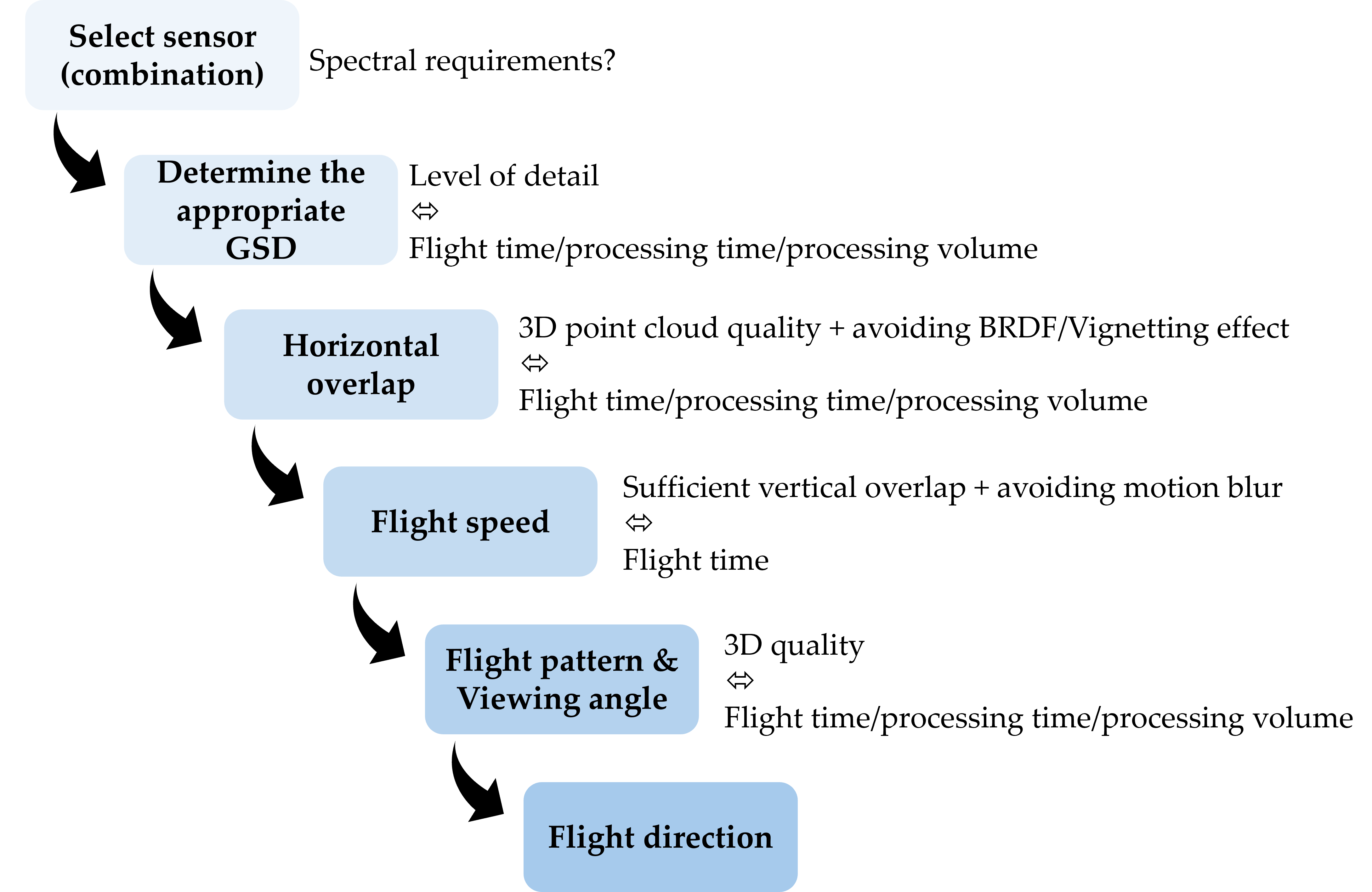
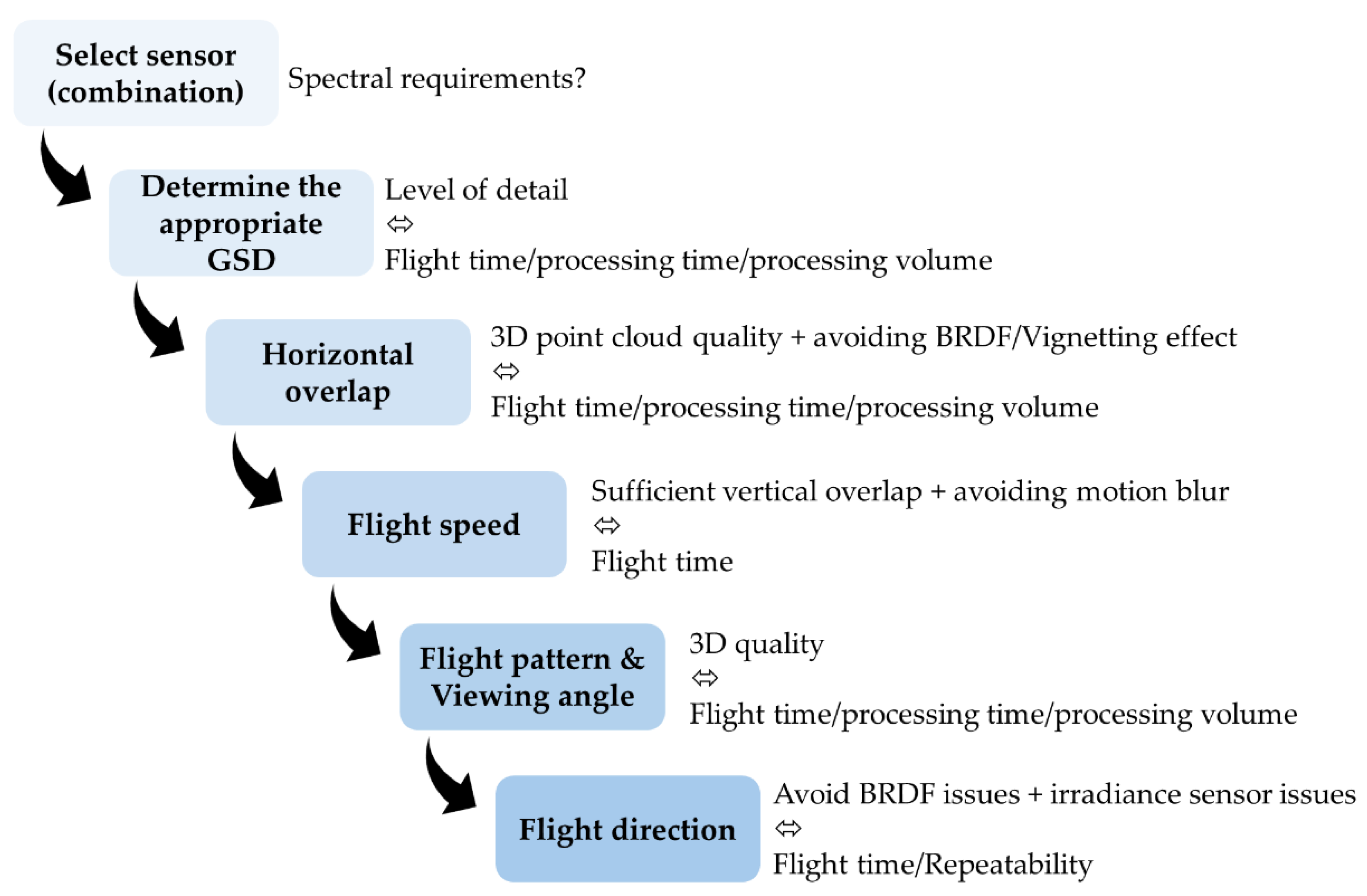
The proper configuration of these parameters is essential, as it directly impacts the quality of the orthomosaic [13]. This section provides guidelines for setting these parameters, emphasizing the balance between detail and quality on one hand, and feasibility on the other. Feasibility involves considerations such as sensor capabilities, flight time, processing time, and data volume. A step-by-step workflow is illustrated in Figure 4; Table 1 summarizes the main recommendations for different sensors at each step.
Figure 4.
General workflow for the flight planning with an indication of the most important considerations in each step.
Figure 4.
General workflow for the flight planning with an indication of the most important considerations in each step.
3.1. Selection of Sensors and Lenses
The first stage of flight preparation involves selecting the appropriate sensor type (e.g., RGB, multispectral, hyperspectral, thermal) or sensor combination, as well as the UAV platform. This decision ultimately depends on the specific application and research objectives. Several reviews, such as those by Aasen et al. [28] and Maes and Steppe [2], provide comprehensive overviews of the advantages and disadvantages of each sensor type. In general, the highest spatial resolution is achieved with RGB cameras and the highest spectral resolution with multi- and hyperspectral sensors.
Particularly for RGB cameras, the sensor resolution is considered the most important camera quality parameter by many. However, it is only one aspect influencing the overall camera quality. Additional factors affecting include image stabilization (In-body and/or lens-based), focus speed and precision and image vignetting and distortion [13]. The lens-sensor combination significantly influences these parameters.
Lens distortion is a critical factor because it impacts the structure-from-motion process. This can be corrected via software self-calibration during processing, or through pre-calibration by imaging a 2D planar reference pattern from different angles (preferred for RGB and thermal cameras - [30,31]). Lens vignetting is less significant for photogrammetry since it can be corrected during post-processing. Structure-from-motion software typically uses the central part of images, especially in standard nadir flights. However, sufficient overlap (Section 3.3) is required to avoid vignetting impact orthomosaic quality.
The focal length is usually expressed in mm and determines, along with the sensor size, the camera’s field of view of the camera – where a larger value represents a more narrow field of view. The selection of the best focal length is not straightforward:
- In general, ultra-wide focal length (<20mm) should be avoided due to significant distortion issues [32].
- Wide lenses (20-40mm) generally show superior photogrammetry results [32,33]. With terrestrial laser scans as reference, Denter et al. [32] compared various lenses for reconstructing a 3D forest scene and found that 21mm and 35mm lenses performed best, as they provided a better lateral view of tree crowns and trunks. Similar results were reported for thermal cameras [34]. On the other hand, the broad range of viewing angles capture within a single image can lead to bidirectional reflectance distribution function (BRDF) issues [25,26] (Section 2), requiring higher overlap (Section 3.3).
- Longer focal lengths (e.g., 50-100mm) produced poorer photogrammetry results than wide-angle cameras, but on the other hand show less distortion and enable lower ground sampling distances for resolutions in the sub-cm or sub-mm range (Section 3.2).
Overall, surprisingly little attention has been given to camera and lens quality specifications and requirements for UAV photogrammetry. O’Connor et al. [12] already argued that many studies fail to report camera specifications and settings in sufficient detail. For an overview of RGB UAV camera considerations, see O’Connor et al. [12] and Roth et al. [13]. Camera settings will are discussed in Section 4.4.
3.2. Ground Sampling Distance and Flight Height
One of the most important mapping flight parameters to consider is the required spatial resolution or ground sampling distance (GSD). Although these terms are often used interchangeably, they have distinct meanings. GSD refers to the distance between the centres of two adjacent pixels, while spatial resolution describes the smallest feature that can be detected. Spatial resolution should also not be confused with camera or sensor resolution, which represents the total number of pixels in a sensor, typically expressed in megapixels.
From this equation, it follows that GSD is determined by camera properties and flight height. This relationship imposes limits on the minimal achievable GSD for a particular sensor-lens combination. Most flight apps set a minimum flight height (e.g., 12 m in DJI apps), effectively determining the smallest achievable GSD. However, lower flight altitudes can be programmed manually using waypoint flight settings, though even then, a minimum flight height must be maintained. For larger UAVs, this limitation is particularly important to prevent collisions with vegetation or structures, as well as to mitigate the effects of downwash. Downwash not only creates unstable flight conditions but can also disturb the canopy or stir up dust and soil affecting image quality [35].
Nevertheless, recent camera and UAV advancements have significantly improved achievable GSD, with sub-millimetre resolution now possible. For example, Van De Vijver et al. [36] achieved a GSD of 0.32 mm, referring to this as "ultra-high resolution." Ultra-high and high resolution have become increasingly relevant, especially in agricultural research, where applications include weed detection [e.g., 37,38], crop emergence monitoring [39,40], ear or flower counting [41,42,43] or plant disease detection [36,44,45]. In ecological studies, applications of high or ultra-high resolution data include flower counting or identification [46,47,48] and tree species mapping [49].
The impact of GSD on data usability is illustrated by RGB imagery of weeds in a cornfield, as shown in Figure 5. At 1mm, 2mm, and possibly 5mm, individual weed species can be identified. At a resolution of 1 cm or 2 cm, weeds between crop rows can still be detected as weeds, but the detail is insufficient for species identification. At 5 cm resolution, the data becomes too coarse for effective weed mapping.
Low GSD (i.e., high resolution) has other benefits, too. High resolution imagery, acquired at lower flight height, generally leads to better 3D reconstruction [50]. Seifert et al. [51] found a hyperbolic increase of the amount of tie points, and hence, of the quality of the 3D model, in the structure-from-motion process with a decrease in flight height.
For multispectral, hyperspectral, and thermal imagery, sensor resolution is typically much lower, resulting in a coarser minimal GSD. Despite this limitation, achieving a low GSD (high resolution) can still be highly beneficial, as it enhances structural detail capture [52], reduces the occurrence of mixed pixels and can improve quality of the orthomosaic [50].
While low GSD offers numerous advantages, it also presents several challenges and limitations. First, achieving high-resolution RGB data is associated with significant resource and logistical costs. It requires advanced equipment, including superior cameras, longer lenses, and heavier UAV platforms. These technological demands translate into greater financial investment.
Second, higher resolution does not always guarantee better results, particularly in interpreting vegetation indices. For example, although some studies found that higher resolution performed best for estimating vegetation characteristics in multispectral imagery (e.g., Zhu et al. [53] for the estimation of biomass in wheat), this is certainly not universally applicable [50,54,55]. Yin et al. [56], for instance, found that multispectral images with a GSD of 2.1 cm were more suitable for predicting SPAD values in winter wheat than those with a finer GSD of 1.1 cm.
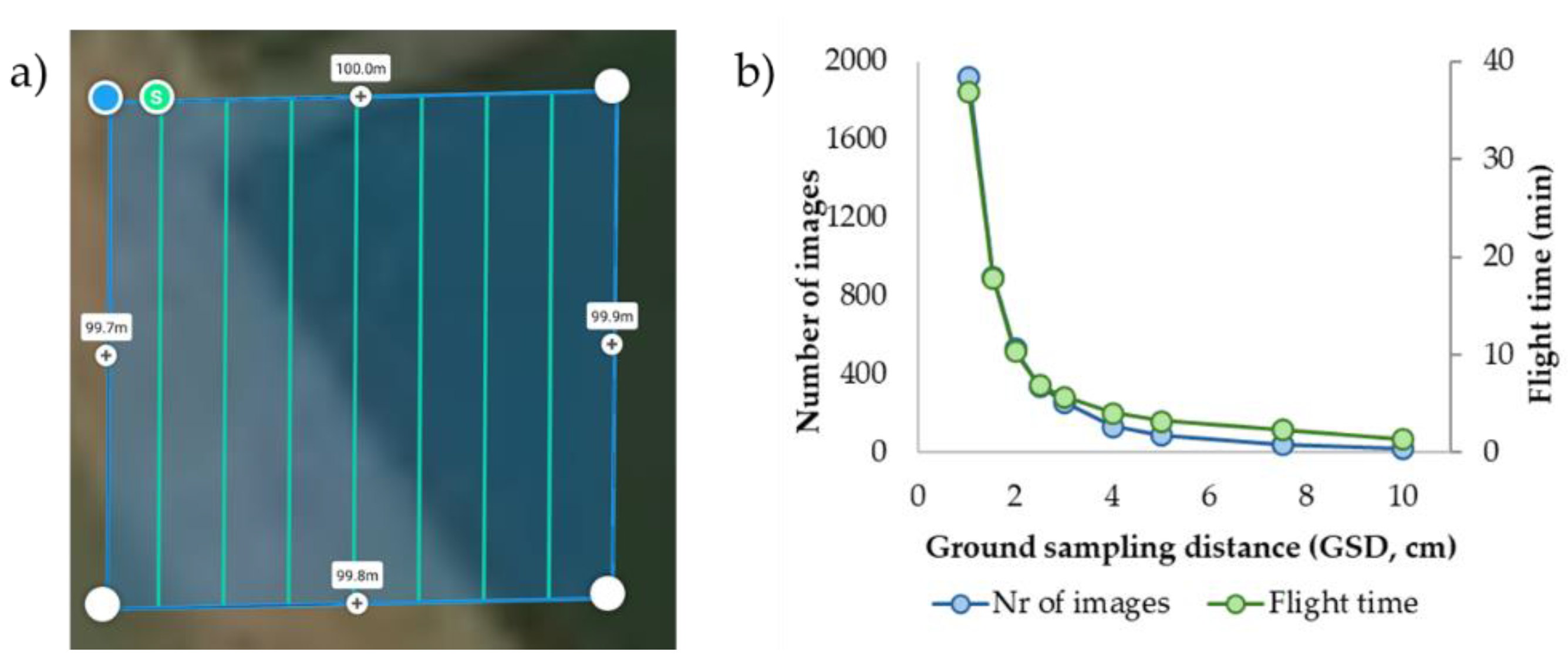
Additionally, the impact of GSD on flight time can be striking. This is a result of longer overall flight paths due to the increased number of flight lines required (Section 3.3) in combination with slower flight speeds (as discussed in Section 3.4). Figure 6b illustrates the relationship between GSD and flight time for a hypothetical area of 1 hectare (100 m × 100 m, Figure 6a) using a standard multispectral camera. At a resolution of 5 cm, the area can be surveyed in 3 minutes and 18 seconds, requiring 90 images and approximately 4.52 GB of storage. Reducing the GSD to 1 cm, however, increases the flight time to nearly 37 minutes, with 2217 images totalling 50.88 GB. Halving the GSD—for example, from 2 cm to 1 cm—increases flight time by a factor of approximately 3.55.
Longer flight durations not only strain resources but also impact data quality. Extended flight times make it more likely for weather conditions to change during the operation, potentially compromising the consistency and reliability of the collected data.
Decreasing the GSD also leads to a significant rise in processing time [51]. Additionally, the size of the final orthomosaic grows exponentially as the GSD decreases. Halving the GSD results in a fourfold increase in the size of the orthomosaic. For example, in the RGB weed dataset illustrated in Figure 5, an 8-bit RGB orthomosaic of a 1-hectare area requires 14.3 MB at 5 cm resolution. This increases to 1.50 GB at 5 mm, 9.51 GB at 2 mm, and 37.7 GB at 1 mm GSD.
This all underscores the critical importance of carefully balancing the desired level of detail against the practical and financial constraints of data collection.
Figure 6.
a) The 1 ha-field of which the simulation was done; b) The effect of GSD on the estimated flight time and the number of images required. Here, we calculated the flight time and number of images of an area of 100m x 100m (1ha) for a multispectral camera (MicaSense RedEdge-MX Dual). The simulation was performed using DJI Pilot app, with settings of horizontal and vertical overlap set at 80%, and the maximum flight speed set at 5m s-1.
The terrain-following option should also be considered when determining the flight height. Terrain following ensures a consistent distance between the UAV and the ground surface, providing a uniform GSD, minimizing out-of-focus issues, and enhancing safety—especially in mountainous regions [57]. True terrain-following can be achieved by equipping a UAV with a laser altimeter, enabling it to maintain a set distance from the ground. While this method is supported by flight apps as UgCS 5, it is primarily designed for low-altitude flights over areas with little or no vegetation and is not yet widely used in mapping applications. Newer UAV models, like the DJI Mavic 3 Enterprise series, offer real-time terrain-following capabilities using obstacle-avoidance cameras, although this feature is currently limited to a minimum flight height of 80 meters.
For other cases, most mapping flight apps now include terrain-following options based on UAV GNSS location and a digital surface model (DSM). Recent flight apps, such as UgCS 4.3 or higher and DJI Pilot 2, integrated DSMs directly, although these often have limited resolution (e.g., 30 meters for DJI Pilot 2 using ASTER DGEM). If higher resolution is needed, users can upload their own DSMs, though this process is less user-friendly and requires additional preparation.
Some studies have successfully applied terrain following [57,58], but there have been no published comparisons of its impact on orthomosaic quality versus the standard constant-altitude approach. Yet, despite the relatively recent introduction of terrain-following features, they are likely to become standard in the near future. In mountainous areas or regions with steep slopes, terrain following should be considered essential. In other areas, it can enhance data quality but is not strictly necessary.
If working in hilly terrain and if terrain-following options are unavailable, it is advisable to take off from a higher point in the landscape whenever possible. This approach improves safety by providing better oversight and reducing the risk of collisions with upslope obstacles, such as trees or buildings. It also helps ensure sufficient overlap in the imagery. When taking off from a higher point is not feasible, a sufficient safety margin in flight height should be maintained, which may require accepting a higher GSD. Adjustments to overlap settings (Section 3.3) should also be made to account for variations in terrain elevation.
3.3. Overlap: Balancing Flight Time and Data Quality
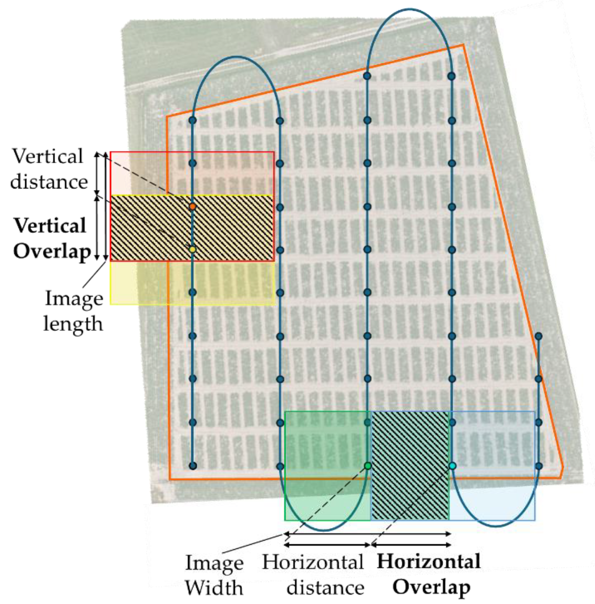
After selecting the camera and determining the GSD, the next crucial parameter to establish is the overlap. Overlap refers to the shared area between two images and can be classified into two types: vertical and horizontal overlap (Figure 7). Vertical overlap pertains to consecutive images captured along the same flight line, while horizontal overlap relates to images captured on adjacent parallel lines.
Vertical overlap is determined by the frequency of image capture and the flight speed, considering the vertical field of view of the camera and the flight height. Mathematically, it can be expressed as (Figure 7):
Here, the "Image length" represents the projected vertical length of an image on the ground, and "Vertical distance" is the spacing between consecutive image captures.
Horizontal overlap, on the other hand, is defined by the distance between two adjacent flight lines and is calculated using the formula:
Where "Image width" is the projected horizontal width of the image, and "Horizontal distance" represents the separation between adjacent flight paths.
Both vertical and horizontal overlap are critical for successful image alignment and mosaicking during the structure-from-motion (SfM) process. They ensure that sufficient tie points exist between images, minimizing geometric errors and improving the accuracy of the final orthomosaic [50,59]. Among these two, vertical overlap is generally the more significant factor influencing orthomosaic quality [50,60]. High vertical overlap (>80%) is now achievable with most sensors, thanks to advancements in image capture frequency.
However, as with flight height, increasing overlap comes at a cost. Greater overlap leads to an hyperbolic rise in the number of images collected, resulting in longer flight times (Figure 8). This, in turn, translates into extended data processing durations and increased resource demands [51,61]. Balancing overlap settings with operational efficiency is therefore essential to optimize both data quality and practical feasibility.
Figure 7.
Schematic figure of a standard (parallel) mapping mission over a target area (orange line) with the planned locations for image capture (dots) illustrating the vertical and horizontal overlap.
Figure 7.
Schematic figure of a standard (parallel) mapping mission over a target area (orange line) with the planned locations for image capture (dots) illustrating the vertical and horizontal overlap.
As such, horizontal and vertical overlap are pivotal parameters to set for UAV imaging, and numerous studies have explored optimal overlap settings. However, these studies often reach differing conclusions, which is not surprising given that overlap and its effects are closely tied to the field of view (or viewing angle) of the sensors. Furthermore, the specific objective defines the optimal overlap.
For generating a geometrically accurate orthomosaic, relatively low overlap values—such as 60% vertical and 50% horizontal—are typically sufficient [31,62]. Similarly, overlaps of 70% vertical and 50% horizontal are generally adequate for creating digital terrain models [59,61]. However, when the goal is to assess the 3D structure and canopy properties of orchard trees or forests, higher overlaps improve the quality of image alignment, tie points, and 3D representations, at the expense of significantly increased processing times [50,60,63,64]. Studies that consider processing efficiency have noted that the marginal quality improvements from extremely high overlap often do not justify the much longer processing times [60,64]. A general consensus here is that for reliable 3D structure reconstruction of trees and forest canopies, vertical overlap should be at least 80% [50,63], while horizontal overlap should be at least 70% [50,51,60]. To map the canopy floor as well, higher overlaps of up to 90% may be necessary [63].
An important consideration in forested or orchard areas is that overlap is typically calculated from the take-off or "home point" level. However, the critical overlap is required at the top of the canopy. Most flight planning apps do not automatically adjust for this, so users must input higher overlap values to ensure adequate coverage at canopy height. This adjustment can be calculated using the formula:
Where OLtarget is the targeted overlap (horizontal or vertical) at the tree top level, OLadj the adjusted overlap (input in the app, overlap at ground level), FH the flight height and VH the vegetation height. This correction becomes more pronounced at lower flight heights and for taller vegetation (Figure 9). For instance, if the targeted overlap at the canopy top is 80%, the adjusted overlap at ground level may need to reach 90% for lower flight altitudes and higher vegetation.
Notably, many studies discussing overlap appear not to have accounted for this correction, which could partially explain the inconsistencies in their overlap recommendations. To facilitate this adjustment, an Excel-based calculator has been provided as supporting information. In sloped areas and if the terrain-follow feature is not activated (see Section 3.2), the actual overlap decreases at higher elevations within the flight area. Equation 4 can be applied here as well to adjust for this discrepancy. Again, a practical solution in such cases is to take off and land from the highest part of the area whenever feasible. This strategy helps maintain consistent overlap, ensuring optimal image alignment and mosaic quality.
For multispectral and hyperspectral imaging, avoiding bidirectional reflectance distribution function (BRDF) effects is critical (Section 2). Higher overlaps reduce the area sampled per image during orthomosaic creation, resulting in a relatively homogeneous orthomosaic (Figure 10). This mitigates deviations in reflectance or surface temperature caused by BRDF effects. The need for higher overlap depends on the viewing angle of the camera; wider viewing angles necessitate greater overlap. A general rule of thumb for typical wide-angle multispectral cameras is to aim for at least 75% vertical and horizontal overlap, and ideally 80% where feasible. If the solar zenith angle is high and hotspots appear in the images, higher overlaps are required to minimize their impact on the orthomosaic. For thermal cameras, the literature is less extensive. However, both BRDF effects and image vignetting can introduce artifacts in thermal orthomosaics, particularly when overlap is insufficient [24,65]. Most radiometric cameras include non-uniformity correction (NUC) to address vignetting issues, but NUC alone may not fully resolve the issue [24,66]. To minimize these effects, a high overlap of 80% in both vertical and horizontal directions is recommended for thermal cameras [67].
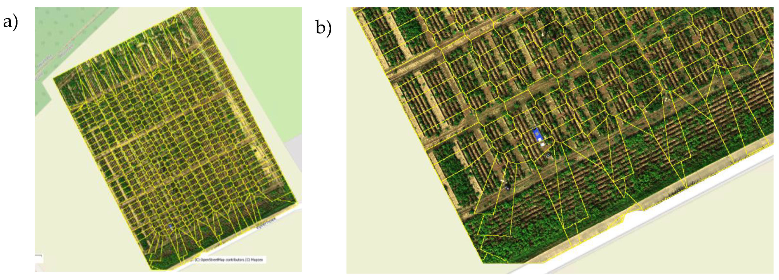
Figure 10.
Orthomosaic of a flight generated with a flight overlap of 80% in horizontal and vertical direction. The yellow lines indicate the area taken from each single image. Notice the constant pattern in the core of the images, whereas the edges typically have larger areas from a single image, increasing the risk of anisotropic effects. A) full field; B) detail. Image taken from Agisoft Metashape from a dataset of multispectral imagery (MicaSense RedEdge-MX Dual), acquired on 07/10/2024, over a potato field in Bottelare Belgium, at a flight altitude of 32m.
3.4. Flight Speed
Flight speed directly influences the area that can be covered during a UAV operation. The maximum allowable flight speed is primarily determined by legal flight speed regulations, the vertical overlap and the frequency of image capture [13]. However, other factors often necessitate a reduction in this speed to ensure image quality and safety.
The most critical consideration is motion blur, which occurs when the UAV (and with it, the camera) moves while the aperture is open. Motion blur reduces image sharpness and detail, potentially impacting the photogrammetric process [68]. This issue is especially pertinent for (ultra) high-resolution RGB imagery. For instance, at a flight speed of 2 m/s and a shutter speed of 1/500th of a second, the UAV moves 4 mm during exposure, which can introduce noticeable blur.
Motion blur is typically expressed as a percentage of the ground sampling distance. While early recommendations suggested keeping motion blur below 150% [12], Roth et al. [13] advocated for stricter limits, recommending it be kept below 50%. Modern cameras often incorporate image stabilization in their sensors or lenses, effectively mitigating motion blur. Additionally, adjusting camera settings, such as increasing shutter speed and compensating with lower aperture or higher ISO (see Section 4.4), can help reduce blur.
Thermal cameras are particularly sensitive to motion blur, despite their generally lower GSD [69]. The microbolometer sensors used in thermal cameras operate differently from photon detectors. Incoming radiation heats the amorphous silicon membrane of each pixel, altering its resistance, which is measured to produce the thermal image. This process has a time lag, defined by the camera's time constant (typically 7–12 ms). As a rule of thumb, it requires about three to five times the time constant for a measurement to reach a steady state and obtain unblurred images. In practice, this is equivalent to a photon camera with a "shutter speed" of around 0.021 seconds (7 ms time * 3 cycles). Even at a modest flight speed of 3 m/s, this results in significant motion blur of approximately 6.3 cm. Despite frequent references to motion blur challenges in thermal UAV imagery [34], there is a lack of studies on the effects of flight speed on thermal image quality or specific recommendations for optimal (maximum) speed.
Higher flight speeds can also increase the UAV’s pitch angle [50]. If the camera is not mounted on a gimbal, this tilt can degrade image quality by causing uneven capture angles.
3.5. Flight Pattern and Flight Direction
Grid flight patterns, where a second set of parallel lines is flown perpendicular to the standard set, have shown potential benefits in specific scenarios. Grid patterns are particularly beneficial for generating accurate point clouds and 3D models, as they allow for lower flight overlap while increasing precision [50,59,70]. Additionally, Asmann et al. [14] suggested that grid patterns may reduce anisotropic effects in multispectral imagery, especially at the edges. However, compelling evidence for this effect remains lacking. Due to the increased flight time, memory requirements, and processing demands, grid patterns are best reserved for applications that require precise digital surface models (DSMs) rather than for general mapping tasks.
The flight direction of the standard parallel flight lines is typically set by the flight app to minimize the flight time. However, users can modify the direction, and certain factors may influence this choice.
One key consideration is wind speed. In windy conditions, headwinds can reduce flight time [71]. However, it is unclear whether flying with a constant sidewind (perpendicular to the wind) is more energy-efficient than alternating between tail- and headwinds.
A more important factor is the sun’s azimuth angle, which affects both the performance of the camera and the incoming light sensor for multispectral systems. Studies have shown that the incoming light sensors of MicaSense DLS2 [17,72] and Parrot Sequoia [73,74,75] are sensitive to their orientation relative to the sun [26].
Jafarbiglu and Pourreza [17] therefor recommended flying perpendicular to the sun direction for the Micasense sensors, in order to minimize these fluctuations. A good – yet untested- alternative can also be to maintain a fixed flight direction (heading) throughout the flight.
Flights should also be planned to minimize anisotropic effects caused by the sun-sensor geometry (Section 2), hotspots in particular should be avoided [17,18]. However, it is not clear whether the flight directions should also be perpendicular to the sun– in fact, as the horizontal field of view of most cameras is typically larger than the vertical field of view, flying parallel to the sun’s azimuth may be more effective.
For reflectance measurements over aquatic systems, special attention is needed to minimize skyglint and sunglint. Mobley [76] recommended flying at a relative azimuth angle of 135° with a viewing angle of 40° to reduce skyglint.
3.6. Viewing Angle
In standard mapping flights, the camera is typically oriented in a nadir-looking position, with its central axis (i.e., the central pixel) perpendicular to the ground. However, most flight apps now offer the option for additional oblique photography, where the camera captures images at an angle. These images are often taken from multiple flight directions and angles. The primary advantage of oblique photography is its ability to improve the quality of digital surface models (DSMs), particularly for vertical structures [77] or trees [78].
Oblique imagery is especially beneficial for terrains with highly variable relief, as it provides more comprehensive coverage of the terrain's vertical and sloping features [79,80,81]. Additionally, it can mitigate the well-known doming effect in structure-from-motion (SfM) models [81,82]. This is likely why DJI Pilot2 incorporates a diagonal flight line with oblique imagery at the end of each standard nadir-flight.
However, the inclusion of oblique photography—particularly from multiple viewing directions—substantially increases flight time, image number, and processing time, following a hyperbolic trend. As such, for applications where 3D point clouds or detailed shape reconstructions are not the primary focus, oblique imagery is generally unnecessary.
That said, oblique imagery has relevance beyond DSM generation. It is particularly useful in studies examining the anisotropy of soils [83] or vegetation [84,85,86,87]. By capturing surface features under varying angles, oblique photography can provide insights into directional patterns of reflectance or structure that are not apparent in nadir imagery.
3.7. Line of Sight Limitation: How Far Can You See a UAV?
In most countries, the legal flight distance for UAVs is restricted to the visual line of sight (VLOS). This means the UAV must remain within the pilot's visible range during the mission. In some jurisdictions, this range can be extended by using UAV spotters, who assist the pilot in maintaining visual contact with the UAV.
So how far can you see a UAV? The detectability of a UAV depends on its size, contrast against the background, and the observer's visual acuity. Li et al. [88] investigated this by determining the probability of detecting a DJI Phantom 4 at various distances. Using a detection probability of 50% as the threshold, they established the maximum visual distance for the Phantom 4 at 245 m, corresponding to a visual angle of 0.065°. A similar study on the DJI Mavic Air found a slightly larger detection range of 307 m, corresponding to the same visual angle [89]. Based on these results, the visual line of sight (VLOS) can be estimated using the formula:
with H the height of the system (m).
VLOS = 881.4 H
EASA, the European Union Aviation Safety Agency responsible for UAV guidelines and legislation, distinguishes two threshold distances, the detection line of sight (DLOS) and the attitude line of sight (ALOS) [90]. The DLOS is the maximum distance at which another aircraft can be visually detected in time to execute an avoidance manoeuvre and is simply given as 30% of the ground visibility. The ALOS is the distance at which the pilot can discern the UAV's position and heading and is for a multicopter calculated as
with CD the characteristic dimension (maximum dimension in m, in this case the diagonal size) of the UAV.
ALOS = 327 CD + 20
Table 2 presents a comparison of visual line-of-sight distances calculated using Equations 5 and 6 for a selection of commonly used UAVs. The two methods show strong agreement (R² = 0.99), with the EASA formula generally yielding slightly longer distances for smaller UAVs and shorter distances for larger ones.
Apart from the UAV's dimensions and the general visibility conditions, obstacles such as trees, buildings, and other structures between the observer and the UAV can affect the visual line of sight. These obstructions may block the view entirely or partially, depending on their size and density, limiting the effective range of VLOS. Additionally, the background contrast plays a crucial role in detecting a UAV. A UAV is much easier to spot when it is flying against a bright background, such as a clear sky, compared to darker backgrounds like dense forests, mountains, or tall buildings. The ability to detect the UAV can therefore vary greatly depending on the landscape and environmental conditions in the flight area.
4. Flight Execution: Ensuring Safe Flights at Best Quality
This section provides an overview of the different aspects to take into account during the flight execution. Table 3 provides a summary for the different camera types.
4.1. Weather Conditions and Their Impact on UAV Mapping Flights
It goes without saying that, as for any UAV flight, the UAV-specific safety restrictions must be respected at all times when performing mapping flights – i.e., pilots should check for maximum wind velocity, kP index, chance of rain, etc for every flight. In addition to these general UAV safety-based limitations, weather condition also influence the quality of the data product, which is the focus of this section.
4.1.1. Illumination
The most critical weather condition for UAV-based remote sensing is incoming solar radiation. Ideally, flights should be conducted under uninterrupted sunny conditions, as these ensure optimal data quality. While patience is often required to wait for such conditions, sunny weather minimizes variability in reflectance and thermal data.
When flying in ideal sunny conditions is not possible, the extent to which overcast or changing conditions affect data quality depends on the sensor type and intended application. For 3D construction with RGB cameras, Slade et al. [91] found that illumination conditions did not have a large influence for 3D construction of trees – in fact, overcast conditions can give slightly better results due to the absence of dark shadows.
For deep learning of high resolution RGB mapping, studies have shown that diverse weather conditions (sunny, overcast, variable) do not significantly affect model outcomes for applications such as weed or disease detection [37,44,92]. Including varied conditions in training datasets is recommended to build robust models.
For multispectral and hyperspectral reflectance measurements, there is more concern. Overcast conditions reduce available light, leading to noisier data, particularly in hyperspectral imaging [93,94]. Further, under overcast conditions, diffuse radiation increases, which has an impact on the reflectance. However, these effects are relatively small [72], particularly when used for vegetation indices [95,96].
Reflectance is defined as the portion of the incoming energy (irradiance) that is reflected per wavelength; hence, variation in irradiance during the flight has a strong effect and must be corrected for [75]. While most multispectral cameras include onboard irradiance sensors, these are, as mentioned in Section 3.5, not always reliable.
Alternative irradiance correction methods exist. Radiometric block adjustment, developed for UAVs by Honkavaara and her team [26,97], compares adjacent images to correct for illumination changes and BRDF effects. This proved to be a more effective than using the on-board irradiance radiometer [26,98,99]. The Retinex method separates reflectance and illumination components via Gaussian filters, and has been successful for estimating chlorophyll in soybean [100] and LAI in rice [101] in varying conditions. Kizel et al. [102] and Qin et al. [103] offer further alternatives for correcting illumination effects. A comparison of these methods, and their implementation in structure-from-motion software deserves further attention.
To conclude, when illumination conditions are suboptimal, it is better to collect data than not to fly at all. A good strategy is to perform an initial flight under varying conditiosn, wait for improved conditions if possible, and repeat the flight to capture higher-quality data.
Thermal imaging is highly sensitive to weather conditions. While cloudy conditions reduce emissivity-related errors [104,105], they also lower contrast and increase noise, complicating the calculation of indices like the Crop Water Stress Index [106,107]. Changes in lighting are challenging to correct in thermal data. Techniques like radiometric block adjustment may offer potential solutions, though they remain underexplored in thermal contexts.
4.1.2. Wind Speed and Air Temperature
Strong wind significantly reduces flight time [71]. Furthermore, strong and variable wind speed affects canopy reconstruction, reducing the accuracy in tree height estimates [91,108]. Strong and variable wind speed also has a limited impact on reflectance data, by affecting leaf angle distribution – although no studies focused specifically on the effect of wind speed on reflectance measurements. Aquatic monitoring can suffer from sunglint issues caused by wind-induced waves [109,110].
Thermal imaging is particularly vulnerable to wind and temperature changes. Increased wind reduces the resistance to heat transport and hence the surface temperature [104]. In general, temperature contrasts are larger at low winds speed. Variable wind speeds can lead to within-flight errors of up to 3.9°C [111] and are difficult to correct for.
4.2. Time of the Flight
The classic remote sensing textbooks generally recommended to perform reflectance measurements around solar noon [e.g., 113,114]. This time of day is characterized by maximum and stable solar intensity, as well as minimal shadow effects, making it ideal for capturing accurate data. In aquatic research, sunglint is also lowest around solar noon [115]. Similarly, thermal remote sensing also benefits from solar noon measurements due to minimized shading, a finding supported by both theoretical and experimental studies [104,116,117]. For high-resolution RGB imaging and the construction of 3D models using structure-from-motion (SfM) software, particularly when focusing on vertical structures, solar noon remains the most favourable time due to the reduced impact of shadows [50]. However, in cases where shadowing is less critical, the time of flight appears less influential for DSM construction [91,108]. Slade et al. [91] even suggest prioritizing flights for mapping vegetation structure during low wind speeds, which often occur earlier in the day, over adhering strictly to solar noon conditions.
The specific purpose of the UAV flight should also guide the choice of optimal flight time. For example, early morning flights are ideal for thermal imagery aimed at wildlife detection because of the pronounced temperature contrast between animals and their surroundings at this time [118]. This early contrast also enhances species-level differentiation [119]. Mapping wildflowers in meadows benefits from the reduced shadowing achieved during solar noon flights [120]. However, this timing may exclude flowers that bloom exclusively in the morning.
Solar elevation significantly influences both reflectance and vegetation indices, such as the normalized difference vegetation index (NDVI). Research has shown that NDVI exhibits a distinct daily pattern, with the lowest values typically recorded around solar noon [18,121]. For repeated flights throughout a season, it is advisable to conduct missions consistently at the same hour or, even better, at the same solar zenith angle. It is also crucial to avoid capturing images that include the hotspot. Particularly in tropical regions during the summer, flying at solar noon may exacerbate this issue, making it better to schedule flights at different times [17]. An online tool1 developed by Jafarbiglu and Pourreza [17] provides guidance on the optimal times to fly for a given sensor, location, and date, offering valuable support for flight planning. Although this tool might be a bit too strict—hotspot effects do not always degrade orthomosaic quality and can sometimes be mitigated by increasing image overlap (Section 3.3)—it is a helpful resource for ensuring data quality.
4.3. Ground Control Points
Ground control points (GCPs) are crucial elements in UAV remote sensing, and are needed to enhance camera alignment and georeferencing in the structure-from-motion (SfM) process [31,122]. These points have known geographic coordinates and are designed for easy identification in images. Typically, UAV GCPs are rectangular panels with a 2x2 black-and-white checkerboard pattern, of which the centre point serves as the reference. High-precision GNSS systems, like RTK, are used to measure their positions accurately. For thermal cameras, GCPs made with dark plastic (warm) and aluminium foil (appearing cold) areas are recommended for better visibility [123,124].
While GCPs play a vital role in refining camera alignment, their use is labour-intensive and time-consuming. Deploying GCPs involves distributing them across the survey area, recording their locations, and collecting them post-flight. For repeated surveys, permanent GCPs, such as plastic markers fixed with pegs, are more practical. The manual matching of GCPs in SfM software further adds to the effort.
The necessity, number, and distribution of GCPs depend on the project requirements and study area. Research findings emphasize several key points:
- Minimum requirements: A minimum of five GCPs is required for successful georeferencing [79,128]. For larger areas or areas with complex terrain, additional GCPs are needed [129], in particular to attain high vertical accuracy [130]. The optimal GCP density ultimately depends on the desired accuracy and the complexity of the relief [79].
- Optimal Distribution: The spatial arrangement of GCPs is as critical as their quantity [125,130]. They should cover the entire survey area, ideally distributed stratified or along the field edges [130]. For a minimal setup of five GCPs, a quincunx (die-like) arrangement is recommended [125]. GCPs near edges should be positioned to ensure they are captured by multiple camera views, and GCPs should not be placed too close to each other, as this can complicate manual matching in SfM software, potentially degrading referencing accuracy.
4.4. Camera Set-Up and Camera Settings
For UAV-based imaging, configuring camera settings correctly is crucial to obtaining high-quality data. For RGB cameras, the challenge is to prioritize between short shutter speed (avoiding motion blur), high F-value (sharper; larger depth of view) and low ISO value (low noise levels); see O’Connor et al. [12] and Roth et al. [13] for a more in-depth discussion. In general, low shutter speed is the most important parameter, and should be at least 1/1000th of a second, and less if possible. If the camera and/or lens have excellent image stabilization, this can be somewhat reduced. The ISO speed is the second most important parameter. For the ISO speed, it is essential to determine the maximum acceptable ISO level for the specific camera [13], with full-frame sensor often showing much lower noise values at a given ISO; this level is furthermore case-specific, as for some applications some level of noise is acceptable.
In sunny and constant lighting conditions, setting the camera manually based on its intensity histogram yields the best results [13]. Under variable lighting, using automatic ISO settings ensures proper exposure across images. Over vegetative areas, underexposing by 0.5–1 stop prevents bright objects like flowers from becoming overexposed. White balance should also match the conditions—make sure to set it manually for consistent lighting, and only use auto settings for changing environments. Capturing images in RAW format enhances dynamic range and facilitates post-flight white balance adjustments, though this requires more memory, can reduce capture frequency, and adds post-processing steps.
For focus settings, integrated cameras usually offer three options: continuous autofocus (AFC in DJI equipment), where the focus is adjusted for each single image; Still autofocus, where the camera focuses when triggered and then remains fixed, and Manual focus, where the user sets the fixed focus distance using a slide bar on the screen. Similarly, cameras that are not fully integrated can have these three options, although manual focus means that you will need to set the focus manually on the lens before the flight.
The focus setting choice depends on flight and camera specifics. At higher altitudes with minimal distance variation and wide lenses, still autofocus or manual focus with fixed settings works best. For lower-altitude flights, with variable distances between sensor and objects or with narrow lenses, continuous autofocus is preferable, especially if terrain following is not employed. Multispectral and thermal cameras typically have fixed focus at infinity due to their wide lenses.
Multispectral cameras usually operate in auto-exposure mode. However, recent research suggests that fixed exposure settings reduce radiometric errors, a potential improvement for future applications [131,132]. For thermal cameras, a non-uniformity correction (NUC), also known as flat-field correction, addresses sensor drift and vignetting. It causes the characteristic clicking noise in thermal cameras. While factory recommendations suggest regular NUCs during flights, this process interrupts data collection temporarily. Studies have indicated that thermal drift during typical flights is minimal [133], leading some experts to recommend performing a single NUC before the flight and leaving it off afterward [123]. When possible, triggering NUCs during non-critical moments, such as at the end of flight lines, minimizes data gaps. If unsure, leaving the NUC on while ensuring sufficient image overlap is a safe choice.
Thermal and multispectral cameras require temperature stabilization, which involves turning on the sensor well before the flight. For thermal cameras, this should be done at least 15 minutes beforehand, or longer if possible, as recommended by multiple studies [24,112,133,134]. Multispectral cameras also benefit from similar stabilization periods [74].
4.5. Reference Measurements and Targets
Reference targets play a critical role in ensuring accurate data processing in UAV-based remote sensing, particularly for reflectance and thermal measurements. For reflectance measurements, the empirical line method (ELM) is widely regarded as the standard approach due to its user-friendly application and precision [28,72].
This method involves imaging grey reference panels with known reflectance values in the field to establish a linear relationship between the sensor’s digital number and the known reflectance of the panels, and subsequently applying this calibration to the entire dataset [72].
A few commercial multispectral systems, such Micasense and Sequoia cameras, include a single small grey panel that needs to be imaged before and after each flight, by holding the UAV and its sensor directly above it. Several commercial SfM packages process these reference panel images automatically, although their algorithms are essentially a black-box leading to small differences in reflectance estimates among the packages [72]. In the field, carefully following the manufacturer’s guidelines is crucial, avoiding casting shadow on the grey panel as well as on the incoming light sensor while holding the UAV.
Using this single grey panel is practical but lacks the capability to correct for atmospheric scattering and absorption. The use of a set of larger grey panels, visible from the operational flight height, is recommended in humid conditions (high air temperature or high relative humidity) or for flights at relatively high flight altitude (roughly flight height >50m) [72,74]. The panel size must be sufficient to include ‘pure’ pixels from the panel centre [96]. These panels should have near-Lambertian properties and their reflectance across all wavelengths must be known. In case of self-made reference panels, it is best to measure their reflectance in the field with a spectrometer around the time of the flight [72]. From personal experience, the set of grey panels for terrestrial vegetation or aquatic applications should include:
- Very dark panel, as dark as possible (ideally, about 1% reflectance): A very dark panel is important as reflectance of vegetation and water in most visible spectra is very low (2-4%), and, ideally, the reference panel should have still lower reflectance.
- Medium dark panels: Dark grey (8-10%) and medium-grey (15-20%): It is important to include panels within this range, because of its relevance in the visual regions, because some multispectral cameras tend to saturate over brighter panels when positioned in an otherwise darker surroundings (such as vegetation or soil), particularly for the visible bands. Including this range of panels still facilitates the ELM method for all channels.
- Bright grey panel: 60-75% reflectance: To include brighter areas, and particularly to correctly estimate reflectance of vegetation in the near-infrared.
Optimal placement of these panels is important; they should be located centrally within the target area, in an open space to minimize the effects of in-scattering from surrounding vegetation or structures [135]. Placing several sets of reference panels strategically over the area is even better, as this can help in correcting for variable irradiance [136].
Finally, while ELM is extensively used for multispectral and hyperspectral imagery, RGB sensors can also benefit from grey panels to normalize reflectance data, given the non-linear relationship—typically exponential or cubic—between digital number and reflectance [100]. Alternative approaches, such as the use of atmospheric radiative transfer models, are particularly effective for hyperspectral data but require more complex post-processing workflows [28,137].
For thermal cameras, several kinds of reference targets must be considered, correcting for different kinds of errors:
- The absolute accuracy of a thermal camera is limited. Similar to the ELM of reflectance measurements, cold and warm reference panels with known temperatures can be used to linearly correct the brightness temperature of the image [24,124,138,139]. Typically, (ice-cold) water is used, or very bright (low temperature) and dark (high temperature) reference panels. Han et al. [140] constructed special temperature-controlled reference targets.
- For research on drought stress or evapotranspiration of terrestrial ecosystems, surface temperature is usually expressed as a thermal index, similar to the vegetation indices for reflectance measurements [104]. The most common index, the crop water stress index CWSI [141,142], uses the lowest and highest possible temperature that the vegetation can attain in the given conditions. These temperatures should not be confounded with the low and high temperature panels for the thermal accuracy correction, since it is crucial that these panels correspond to temperatures of the actual vegetation [143,144]. A common reference target is to use a wet cloth as cold reference temperature, as it transpires at maximal rate and essentially provides the wet bulb temperature [124,145,146]. However, it doesn’t accurately represent the canopy conditions [144,147]. Maes et al. [144] showed that artificial leaves made of cotton, remaining wet by constantly absorbing water from a reservoir, gives a more precise estimate, but the scalability of this method to field level remains to be explored.
- Vignetting in thermal cameras can create temperature differences between the edges and the centre of the image of up to several degrees [24]. The non-uniformity correction (NUC, Section 4.4) is for some models not sufficient [24], in which case the vignetting can be quantified by taking a thermal image of a uniform blackbody [24,148]. However, this is not absolutely required, provided that a sufficiently high horizontal and vertical overlap are foreseen.
In addition, some measurement conditions should be recorded. Although other correction methods exist (cfr. Section 4.1), incoming light can best be measured for correction of multispectral or hyperspectral imagery, particularly when conditions are variable. As explained earlier, most multispectral cameras have an incoming light sensor; for hyperspectral cameras, irradiance spectrometers can be used, either on-board the UAV or located at the ground level [28]. For thermal measurements, at least air temperature and relative humidity should be known, to correct for atmospheric conditions [31,112] (cfr. Section 4.1).
5. Discussion
Towards a Universal MAPPING protocol?
This article outlined recommendations for flight planning and execution across a range of UAV-mounted sensors. In reviewing the literature, several knowledge gaps were identified. One prominent area for further investigation is the optimal flight direction relative to the sun's zenith angle as well as the dominant wind speed, which remains insufficiently explored. For thermal imaging, in particular, there is a noticeable scarcity of research addressing the optimization of flight parameters. Unresolved questions for thermal imaging persist regarding the effects of flight altitude and speed on image quality, the determination of optimal overlap, strategies for correcting variations in atmospheric and weather conditions, and the influence of anisotropy (BRDF) effects.
Despite these knowledge gaps, the need for harmonization and standardization in UAV mapping protocols is evident. Standardized approaches are critical for producing repeatable datasets and developing transferable machine learning models. Each application requires specific parameter settings, particularly concerning ground sampling distance (GSD) and flight height, which limits the creation of universally applicable protocols. Nonetheless, adhering to the recommendations summarized in Table 1 and Table 3 could facilitate standardized approaches tailored to specific applications. Inspiration for such protocols can be drawn from initiatives such as TERN Australia's UAV field operation guidelines, which provide structured methodologies for UAV-based data collection2.
Even with rigorous protocols, weather conditions inevitably affect the orthomosaic. These external influences, along with the associated camera settings, are underreported in current literature. To ensure datasets are interpretable and comparable, proper annotation of metadata is essential. Metadata should comprehensively document flight parameters, camera settings, and meteorological conditions during the flight. Developing and adopting a standardized framework for metadata annotation is critical for advancing the field. Such a framework would not only improve data comparability but also foster a shared understanding of UAV-derived datasets within the research community.
Is There an Alternative for the Tedious Flight Mapping and Processing?
While each pixel is captured multiple times from various viewing angles, standard blending techniques typically retain only the most nadir-looking observation for constructing the orthomosaic. As such, the high overlap in UAV mapping flights generates significant "redundant" information. To address this inefficiency, several methods have been proposed to either make better use of the captured data or to reduce the volume of data collected.
One approach to maximizing the utility of the dataset is to use alternative blending modes during orthomosaic creation. For instance, the ‘average’ or weighted average blending mode (e.g., ‘orthomosaic’) has been explored as an alternative to the standard (‘disable’) mode. [94,123]. However, the interpretation of this product is not necessarily more straightforward [123] and neither does the quality of the orthomosaic necessarily improve [65].
A more complex approach involves moving beyond the traditional orthomosaic by incorporating individual directional observations directly into the analysis. Roosjen et al. [87] applied SfM software to extract observations along with their relative azimuth and sensor zenith angles, then used them as input for a radiative transfer model (PROSAIL) to derive plant parameters. This method exemplifies how raw, angular-specific data can provide additional insights, albeit at the cost of greater computational complexity and specialized expertise.
An alternative, simpler strategy with potentially broader applicability was recently introduced by Heim et al. [27]. They developed machine learning models to predict leaf chlorophyll content and leaf area index (LAI) in maize. The study revealed that using all observations from all viewing angles as input led to poorer model performance compared to models trained on standard orthomosaic data. However, selecting observations from a restricted range of sensor zenith and relative azimuth angles significantly enhanced the models’ predictive accuracy relative to the standard orthomosaic.
Reducing data collection volume can be achieved by revising flight planning strategies. Mueller et al. [81] demonstrated that alternative flight trajectories, such as spiral or loop patterns, reduced flight time while yielding better DSM quality compared to traditional mapping with parallel flight lines and nadir-looking cameras. However, this finding was limited to relatively flat, square areas, and further research is required to explore its applicability to diverse terrain types and for data acquisition beyond DSMs, such as reflectance or thermal imagery.
A more transformative alternative is to replace traditional mapping flights with direct sampling flights. The individual images are georeferenced based on the sensor’s (and UAV's) position and attitude at the time of capture, and are then analysed individually. This approach bypasses the SfM processing. Direct sampling has been utilized for some time, for instance in aquatic sensing [110,149], for thermal imagery [150,151], and for high-resolution RGB data [36,44].
However, consumer-grade miniature UAVs could give it a new stimulus. These small UAVs, equipped with high-resolution cameras, can fly at very low altitudes to capture ultra-high resolution images [92,152], for a fraction of the cost of the standard ultra-high resolution UAV system. Their minimal size avoids the downwash disturbances associated with professional UAVs operating at low altitudes (Section 3.2). Many contemporary models also include waypoint flight capabilities, enabling them to be programmed for systematic flights akin to mapping missions, but at much lower altitudes and with no or very low overlap between images [153]. This approach can dramatically reduce flight time, data volume, and post-processing efforts. Additionally, when equipped with RTK GNSS, direct and highly precise georeferencing of the images is feasible [153].
Direct sampling missions for RGB data collection are not yet integrated into standard UAV flight software and present certain safety challenges, such as low-altitude flights and line-of-sight constraints. Nonetheless, they might represent a promising and competitive alternative for high-resolution RGB data collection in the near future. For multispectral/hyperspectral or thermal data, Direct sampling has less potential, given the influence of BRDF and/or vignetting on the image quality.
Supplementary Materials
The following supporting information can be downloaded at the website of this paper posted on Preprints.org, Excel file with calculation of overlap.
Author Contributions
Conceptualization, methodology, formal analysis, writing: W.H.M.
Funding
WHM did not receive special funding for this review.
Conflicts of Interest
The author declares no conflicts of interest.
| 1 | https://digitalag.ucdavis.edu/decision-support-tools/when2fly. |
| 2 | https://www.tern.org.au/data-collection-protocols/. |
References
- Statista. Drones - Worldwide. Available online: https://www.statista.com/outlook/cmo/consumer-electronics/drones/worldwide (accessed on 06/11/2024).
- Maes, W.H.; Steppe, K. Perspectives for remote sensing with Unmanned Aerial Vehicles in precision agriculture. Trends in Plant Science 2019, 24, 45. [Google Scholar] [CrossRef] [PubMed]
- Tang, L.; Shao, G. Drone remote sensing for forestry research and practices. Journal of Forestry Research 2015, 26, 791–797. [Google Scholar] [CrossRef]
- Koh, L.P.; Wich, S.A. Dawn of Drone Ecology: Low-Cost Autonomous Aerial Vehicles for Conservation. Tropical Conservation Science 2012, 5, 121–132. [Google Scholar] [CrossRef]
- Sun, Z.; Wang, X.; Wang, Z.; Yang, L.; Xie, Y.; Huang, Y. UAVs as remote sensing platforms in plant ecology: review of applications and challenges. Journal of Plant Ecology 2021, 14, 1003–1023. [Google Scholar] [CrossRef]
- Mesas-Carrascosa, F.-J.; Notario García, M.D.; Meroño de Larriva, J.E.; García-Ferrer, A. An Analysis of the Influence of Flight Parameters in the Generation of Unmanned Aerial Vehicle (UAV) Orthomosaicks to Survey Archaeological Areas. Sensors 2016, 16, 1838. [Google Scholar] [CrossRef] [PubMed]
- Pepe, M.; Alfio, V.S.; Costantino, D. UAV Platforms and the SfM-MVS Approach in the 3D Surveys and Modelling: A Review in the Cultural Heritage Field. Applied Sciences-Basel 2022, 12. [Google Scholar] [CrossRef]
- Bhardwaj, A.; Sam, L.; Akanksha; Martín-Torres, F.J.; Kumar, R. UAVs as remote sensing platform in glaciology: Present applications and future prospects. Remote Sensing of Environment 2016, 175, 196–204. [CrossRef]
- Park, S.; Choi, Y. Applications of Unmanned Aerial Vehicles in Mining from Exploration to Reclamation: A Review. Minerals 2020, 10. [Google Scholar] [CrossRef]
- Jiang, S.; Jiang, C.; Jiang, W.S. Efficient structure from motion for large-scale UAV images: A review and a comparison of SfM tools. ISPRS Journal of Photogrammetry and Remote Sensing 2020, 167, 230–251. [Google Scholar] [CrossRef]
- Iglhaut, J.; Cabo, C.; Puliti, S.; Piermattei, L.; O'Connor, J.; Rosette, J. Structure from Motion Photogrammetry in Forestry: a Review. Current Forestry Reports 2019, 5, 155–168. [Google Scholar] [CrossRef]
- O’Connor, J.; Smith, M.J.; James, M.R. Cameras and settings for aerial surveys in the geosciences: Optimising image data. Progress in Physical Geography: Earth and Environment 2017, 41, 325–344. [Google Scholar] [CrossRef]
- Roth, L.; Hund, A.; Aasen, H. PhenoFly Planning Tool: flight planning for high-resolution optical remote sensing with unmanned areal systems. Plant Methods 2018, 14, 116. [Google Scholar] [CrossRef] [PubMed]
- Assmann, J.J.; Kerby, J.T.; Cunliffe, A.M.; Myers-Smith, I.H. Vegetation monitoring using multispectral sensors — best practices and lessons learned from high latitudes. Journal of Unmanned Vehicle Systems 2019, 7, 54–75. [Google Scholar] [CrossRef]
- Tmušić, G.; Manfreda, S.; Aasen, H.; James, M.R.; Gonçalves, G.; et al. Current Practices in UAS-based Environmental Monitoring. Remote Sensing 2020, 12, 1001. [Google Scholar] [CrossRef]
- Li, Z.; Roy, D.P.; Zhang, H.K. The incidence and magnitude of the hot-spot bidirectional reflectance distribution function (BRDF) signature in GOES-16 Advanced Baseline Imager (ABI) 10 and 15 minute reflectance over north America. Remote Sensing of Environment 2021, 265, 112638. [Google Scholar] [CrossRef]
- Jafarbiglu, H.; Pourreza, A. Impact of sun-view geometry on canopy spectral reflectance variability. ISPRS Journal of Photogrammetry and Remote Sensing 2023, 196, 270–286. [Google Scholar] [CrossRef]
- Stow, D.; Nichol, C.J.; Wade, T.; Assmann, J.J.; Simpson, G.; Helfter, C. Illumination Geometry and Flying Height Influence Surface Reflectance and NDVI Derived from Multispectral UAS Imagery. Drones 2019, 3, 55. [Google Scholar] [CrossRef]
- Bovend'aerde, L. An empirical BRDF model for the Queensland rainforests. Ghent University, 2016.
- Bian, Z.; Roujean, J.-L.; Cao, B.; Du, Y.; Li, H.; Gamet, P.; Fang, J.; Xiao, Q.; Liu, Q. Modeling the directional anisotropy of fine-scale TIR emissions over tree and crop canopies based on UAV measurements. Remote Sensing of Environment 2021, 252, 112150. [Google Scholar] [CrossRef]
- Bian, Z.; Roujean, J.L.; Lagouarde, J.P.; Cao, B.; Li, H.; Du, Y.; Liu, Q.; Xiao, Q.; Liu, Q. A semi-empirical approach for modeling the vegetation thermal infrared directional anisotropy of canopies based on using vegetation indices. ISPRS Journal of Photogrammetry and Remote Sensing 2020, 160, 136–148. [Google Scholar] [CrossRef]
- Lagouarde, J.P.; Dayau, S.; Moreau, P.; Guyon, D. Directional Anisotropy of Brightness Surface Temperature Over Vineyards: Case Study Over the Medoc Region (SW France). IEEE Geoscience and Remote Sensing Letters 2014, 11, 574–578. [Google Scholar] [CrossRef]
- Jiang, L.; Zhan, W.; Tu, L.; Dong, P.; Wang, S.; Li, L.; Wang, C.; Wang, C. Diurnal variations in directional brightness temperature over urban areas through a multi-angle UAV experiment. Building and Environment 2022, 222, 109408. [Google Scholar] [CrossRef]
- Kelly, J.; Kljun, N.; Olsson, P.-O.; Mihai, L.; Liljeblad, B.; Weslien, P.; Klemedtsson, L.; Eklundh, L. Challenges and Best Practices for Deriving Temperature Data from an Uncalibrated UAV Thermal Infrared Camera. Remote Sensing 2019, 11, 567. [Google Scholar] [CrossRef]
- Stark, B.; Zhao, T.; Chen, Y. An analysis of the effect of the bidirectional reflectance distribution function on remote sensing imagery accuracy from Small Unmanned Aircraft Systems. In 7-10 June 2016, 2016; pp. 1342-1350. 10 June.
- Honkavaara, E.; Khoramshahi, E. Radiometric Correction of Close-Range Spectral Image Blocks Captured Using an Unmanned Aerial Vehicle with a Radiometric Block Adjustment. Remote Sensing 2018, 10, 256. [Google Scholar] [CrossRef]
- Heim, R.H.J.; Okole, N.; Steppe, K.; Van Labeke, M.-C.; Geedicke, I.; Maes, W.H. An applied framework to unlocking multi-angular UAV reflectance data: a case study for classification of plant parameters in maize (Zea mays). Precision Agriculture 2024, 25, 1751–1775. [Google Scholar] [CrossRef]
- Aasen, H.; Honkavaara, E.; Lucieer, A.; Zarco-Tejada, P. Quantitative remote sensing at ultra-high resolution with uav spectroscopy: A review of sensor technology, measurement procedures, and data correction workflows. Remote Sensing 2018, 10, 1091. [Google Scholar] [CrossRef]
- Tu, Y.-H.; Phinn, S.; Johansen, K.; Robson, A. Assessing Radiometric Correction Approaches for Multi-Spectral UAS Imagery for Horticultural Applications. Remote Sensing 2018, 10, 1684. [Google Scholar] [CrossRef]
- Griffiths, D.; Burningham, H. Comparison of pre- and self-calibrated camera calibration models for UAS-derived nadir imagery for a SfM application. Progress in Physical Geography: Earth and Environment 2019, 43, 215–235. [Google Scholar] [CrossRef]
- Maes, W.; Huete, A.; Steppe, K. Optimizing the processing of UAV-based thermal imagery. Remote Sensing 2017, 9, 476. [Google Scholar] [CrossRef]
- Denter, M.; Frey, J.; Kattenborn, T.; Weinacker, H.; Seifert, T.; Koch, B. Assessment of camera focal length influence on canopy reconstruction quality. ISPRS Open Journal of Photogrammetry and Remote Sensing 2022, 6, 100025. [Google Scholar] [CrossRef]
- Kraus, K. Photogrammetry: geometry from images and laser scans; Walter de Gruyter: 2011.
- Sangha, H.S.; Sharda, A.; Koch, L.; Prabhakar, P.; Wang, G. Impact of camera focal length and sUAS flying altitude on spatial crop canopy temperature evaluation. Computers and Electronics in Agriculture 2020, 172, 105344. [Google Scholar] [CrossRef]
- Zhu, Y.; Guo, Q.; Tang, Y.; Zhu, X.; He, Y.; Huang, H.; Luo, S. CFD simulation and measurement of the downwash airflow of a quadrotor plant protection UAV during operation. Computers and Electronics in Agriculture 2022, 201, 107286. [Google Scholar] [CrossRef]
- Van De Vijver, R.; Mertens, K.; Heungens, K.; Nuyttens, D.; Wieme, J.; Maes, W.H.; Van Beek, J.; Somers, B.; Saeys, W. Ultra-High-Resolution UAV-Based Detection of Alternaria solani Infections in Potato Fields. Remote Sensing 2022, 14, 6232. [Google Scholar] [CrossRef]
- Rasmussen, J.; Nielsen, J.; Streibig, J.C.; Jensen, J.E.; Pedersen, K.S.; Olsen, S.I. Pre-harvest weed mapping of Cirsium arvense in wheat and barley with off-the-shelf UAVs. Precision Agriculture 2019, 20, 983–999. [Google Scholar] [CrossRef]
- Gao, J.; Liao, W.; Nuyttens, D.; Lootens, P.; Vangeyte, J.; Pižurica, A.; He, Y.; Pieters, J.G. Fusion of pixel and object-based features for weed mapping using unmanned aerial vehicle imagery. International Journal of Applied Earth Observation and Geoinformation 2018, 67, 43–53. [Google Scholar] [CrossRef]
- Barreto, A.; Lottes, P.; Ispizua Yamati, F.R.; Baumgarten, S.; Wolf, N.A.; Stachniss, C.; Mahlein, A.-K.; Paulus, S. Automatic UAV-based counting of seedlings in sugar-beet field and extension to maize and strawberry. Computers and Electronics in Agriculture 2021, 191, 106493. [Google Scholar] [CrossRef]
- García-Martínez, H.; Flores-Magdaleno, H.; Khalil-Gardezi, A.; Ascencio-Hernández, R.; Tijerina-Chávez, L.; Vázquez-Peña, M.A.; Mancilla-Villa, O.R. Digital Count of Corn Plants Using Images Taken by Unmanned Aerial Vehicles and Cross Correlation of Templates. Agronomy 2020, 10, 469. [Google Scholar] [CrossRef]
- Petti, D.; Li, C.Y. Weakly-supervised learning to automatically count cotton flowers from aerial imagery. Computers and Electronics in Agriculture 2022, 194. [Google Scholar] [CrossRef]
- Xu, X.; Li, H.; Yin, F.; Xi, L.; Qiao, H.; Ma, Z.; Shen, S.; Jiang, B.; Ma, X. Wheat ear counting using K-means clustering segmentation and convolutional neural network. Plant Methods 2020, 16, 106. [Google Scholar] [CrossRef] [PubMed]
- Fernandez-Gallego, J.A.; Lootens, P.; Borra-Serrano, I.; Derycke, V.; Haesaert, G.; Roldán-Ruiz, I.; Araus, J.L.; Kefauver, S.C. Automatic wheat ear counting using machine learning based on RGB UAV imagery. The Plant Journal 2020, 103, 1603–1613. [Google Scholar] [CrossRef] [PubMed]
- Wieme, J.; Leroux, S.; Cool, S.R.; Van Beek, J.; Pieters, J.G.; Maes, W.H. Ultra-high-resolution UAV-imaging and supervised deep learning for accurate detection of Alternaria solani in potato fields. Frontiers in Plant Science 2024, 15. [Google Scholar] [CrossRef]
- Kontogiannis, S.; Konstantinidou, M.; Tsioukas, V.; Pikridas, C. A Cloud-Based Deep Learning Framework for Downy Mildew Detection in Viticulture Using Real-Time Image Acquisition from Embedded Devices and Drones. Information 2024, 15, 178. [Google Scholar] [CrossRef]
- Carl, C.; Landgraf, D.; Van der Maaten-Theunissen, M.; Biber, P.; Pretzsch, H. Robinia pseudoacacia L. Flower Analyzed by Using An Unmanned Aerial Vehicle (UAV). Remote Sensing 2017, 9, 1091. [Google Scholar] [CrossRef]
- Gallmann, J.; Schüpbach, B.; Jacot, K.; Albrecht, M.; Winizki, J.; Kirchgessner, N.; Aasen, H. Flower Mapping in Grasslands With Drones and Deep Learning. Frontiers in Plant Science 2022, 12. [Google Scholar] [CrossRef] [PubMed]
- Gröschler, K.-C.; Muhuri, A.; Roy, S.K.; Oppelt, N. Monitoring the Population Development of Indicator Plants in High Nature Value Grassland Using Machine Learning and Drone Data. Drones 2023, 7, 644. [Google Scholar] [CrossRef]
- Pu, R. Mapping Tree Species Using Advanced Remote Sensing Technologies: A State-of-the-Art Review and Perspective. Journal of Remote Sensing 2021, 2021. [Google Scholar] [CrossRef]
- Tu, Y.-H.; Phinn, S.; Johansen, K.; Robson, A.; Wu, D. Optimising drone flight planning for measuring horticultural tree crop structure. ISPRS Journal of Photogrammetry and Remote Sensing 2020, 160, 83–96. [Google Scholar] [CrossRef]
- Seifert, E.; Seifert, S.; Vogt, H.; Drew, D.; van Aardt, J.; Kunneke, A.; Seifert, T. Influence of Drone Altitude, Image Overlap, and Optical Sensor Resolution on Multi-View Reconstruction of Forest Images. Remote Sensing 2019, 11, 1252. [Google Scholar] [CrossRef]
- Jay, S.; Baret, F.; Dutartre, D.; Malatesta, G.; Héno, S.; Comar, A.; Weiss, M.; Maupas, F. Exploiting the centimeter resolution of UAV multispectral imagery to improve remote-sensing estimates of canopy structure and biochemistry in sugar beet crops. Remote Sensing of Environment 2018. [Google Scholar] [CrossRef]
- Zhu, W.; Rezaei, E.E.; Nouri, H.; Sun, Z.; Li, J.; Yu, D.; Siebert, S. UAV Flight Height Impacts on Wheat Biomass Estimation via Machine and Deep Learning. IEEE Journal of Selected Topics in Applied Earth Observations and Remote Sensing 2023, 16, 7471–7485. [Google Scholar] [CrossRef]
- Avtar, R.; Suab, S.A.; Syukur, M.S.; Korom, A.; Umarhadi, D.A.; Yunus, A.P. Assessing the Influence of UAV Altitude on Extracted Biophysical Parameters of Young Oil Palm. Remote Sensing 2020, 12, 3030. [Google Scholar] [CrossRef]
- Johansen, K.; Raharjo, T.; McCabe, M.F. Using Multi-Spectral UAV Imagery to Extract Tree Crop Structural Properties and Assess Pruning Effects. Remote Sensing 2018, 10, 854. [Google Scholar] [CrossRef]
- Yin, Q.; Zhang, Y.; Li, W.; Wang, J.; Wang, W.; Ahmad, I.; Zhou, G.; Huo, Z. Estimation of Winter Wheat SPAD Values Based on UAV Multispectral Remote Sensing. Remote Sensing 2023, 15, 3595. [Google Scholar] [CrossRef]
- Singh, C.H.; Mishra, V.; Jain, K. High-resolution mapping of forested hills using real-time UAV terrain following. ISPRS Ann. Photogramm. Remote Sens. Spatial Inf. Sci. 2023, X-1/W1-2023, 665-671. [CrossRef]
- Li, Q.; Yao, X.; Li, R.; Zhou, Z.; Yao, C.; Ren, K. Quick Extraction of Joint Surface Attitudes and Slope Preliminary Stability Analysis: A New Method Using Unmanned Aerial Vehicle 3D Photogrammetry and GIS Development. Remote Sensing 2024, 16, 1022. [Google Scholar] [CrossRef]
- Chaudhry, M.H.; Ahmad, A.; Gulzar, Q. Impact of UAV Surveying Parameters on Mixed Urban Landuse Surface Modelling. ISPRS International Journal of Geo-Information 2020, 9, 656. [Google Scholar] [CrossRef]
- Domingo, D.; Ørka, H.O.; Næsset, E.; Kachamba, D.; Gobakken, T. Effects of UAV Image Resolution, Camera Type, and Image Overlap on Accuracy of Biomass Predictions in a Tropical Woodland. Remote Sensing 2019, 11, 948. [Google Scholar] [CrossRef]
- Lopes Bento, N.; Araújo E Silva Ferraz, G.; Alexandre Pena Barata, R.; Santos Santana, L.; Diennevan Souza Barbosa, B.; Conti, L.; Becciolini, V.; Rossi, G. Overlap influence in images obtained by an unmanned aerial vehicle on a digital terrain model of altimetric precision. European Journal of Remote Sensing 2022, 55, 263–276. [Google Scholar] [CrossRef]
- Flores-de-Santiago, F.; Valderrama-Landeros, L.; Rodríguez-Sobreyra, R.; Flores-Verdugo, F. Assessing the effect of flight altitude and overlap on orthoimage generation for UAV estimates of coastal wetlands. Journal of Coastal Conservation 2020, 24, 35. [Google Scholar] [CrossRef]
- Dandois, J.P.; Olano, M.; Ellis, E.C. Optimal Altitude, Overlap, and Weather Conditions for Computer Vision UAV Estimates of Forest Structure. Remote Sensing 2015, 7, 13895–13920. [Google Scholar] [CrossRef]
- Torres-Sánchez, J.; López-Granados, F.; Borra-Serrano, I.; Peña, J.M.J.P.A. Assessing UAV-collected image overlap influence on computation time and digital surface model accuracy in olive orchards. 2018, 19, 115-133. [CrossRef]
- Malbéteau, Y.; Johansen, K.; Aragon, B.; Al-Mashhawari, S.K.; McCabe, M.F. Overcoming the Challenges of Thermal Infrared Orthomosaics Using a Swath-Based Approach to Correct for Dynamic Temperature and Wind Effects. Remote Sensing 2021, 13, 3255. [Google Scholar] [CrossRef]
- Olbrycht, R.; Więcek, B. New approach to thermal drift correction in microbolometer thermal cameras. Quantitative InfraRed Thermography Journal 2015, 12, 184–195. [Google Scholar] [CrossRef]
- Boesch, R. Thermal remote sensing with UAV-based workflows. Int. Arch. Photogramm. Remote Sens. Spatial Inf. Sci. 2017, XLII-2/W6, 41-46. [CrossRef]
- Sieberth, T.; Wackrow, R.; Chandler, J.H. Motion blur disturbs - The influence of motion-blurred images in photogrammetry. Photogrammetric Record 2014, 29, 434–453. [Google Scholar] [CrossRef]
- Lee, K.; Ban, Y.; Kim, C. Motion Blur Kernel Rendering Using an Inertial Sensor: Interpreting the Mechanism of a Thermal Detector. Sensors 2022, 22, 1893. [Google Scholar] [CrossRef] [PubMed]
- Ahmed, S.; El-Shazly, A.; Abed, F.; Ahmed, W. The Influence of Flight Direction and Camera Orientation on the Quality Products of UAV-Based SfM-Photogrammetry. Applied Sciences 2022, 12, 10492. [Google Scholar] [CrossRef]
- Beigi, P.; Rajabi, M.S.; Aghakhani, S. An Overview of Drone Energy Consumption Factors and Models. In Handbook of Smart Energy Systems, Fathi, M., Zio, E., Pardalos, P.M., Eds.; Springer International Publishing: Cham, 2021; pp. 1–20. [Google Scholar]
- Daniels, L.; Eeckhout, E.; Wieme, J.; Dejaegher, Y.; Audenaert, K.; Maes, W.H. Identifying the Optimal Radiometric Calibration Method for UAV-Based Multispectral Imaging. Remote Sensing 2023, 15, 2909. [Google Scholar] [CrossRef]
- Fawcett, D.; Anderson, K. Investigating impacts of calibration methodology and irradiance variations on lightweight drone-based sensor derived surface reflectance products; SPIE: 2019; Volume 11149.
- Olsson, P.-O.; Vivekar, A.; Adler, K.; Garcia Millan, V.E.; Koc, A.; Alamrani, M.; Eklundh, L. Radiometric Correction of Multispectral UAS Images: Evaluating the Accuracy of the Parrot Sequoia Camera and Sunshine Sensor. Remote Sensing 2021, 13, 577. [Google Scholar] [CrossRef]
- Zhu, H.; Huang, Y.; An, Z.; Zhang, H.; Han, Y.; Zhao, Z.; Li, F.; Zhang, C.; Hou, C. Assessing radiometric calibration methods for multispectral UAV imagery and the influence of illumination, flight altitude and flight time on reflectance, vegetation index and inversion of winter wheat AGB and LAI. Computers and Electronics in Agriculture 2024, 219, 108821. [Google Scholar] [CrossRef]
- Mobley, C.D. Estimation of the remote-sensing reflectance from above-surface measurements. Appl. Opt. 1999, 38, 7442–7455. [Google Scholar] [CrossRef] [PubMed]
- Jiang, S.; Jiang, W.; Huang, W.; Yang, L. UAV-based oblique photogrammetry for outdoor data acquisition and offsite visual inspection of transmission line. Remote Sensing 2017, 9, 278. [Google Scholar] [CrossRef]
- Lin, Y.; Jiang, M.; Yao, Y.; Zhang, L.; Lin, J. Use of UAV oblique imaging for the detection of individual trees in residential environments. Urban forestry & urban greening 2015, 14, 404–412. [Google Scholar]
- Dai, W.; Zheng, G.; Antoniazza, G.; Zhao, F.; Chen, K.; Lu, W.; Lane, S.N. Improving UAV-SfM photogrammetry for modelling high-relief terrain: Image collection strategies and ground control quantity. Earth Surface Processes and Landforms 2023, 48, 2884–2899. [Google Scholar] [CrossRef]
- Nesbit, P.R.; Hugenholtz, C.H. Enhancing UAV–SfM 3D Model Accuracy in High-Relief Landscapes by Incorporating Oblique Images. Remote Sensing 2019, 11, 239. [Google Scholar] [CrossRef]
- Mueller, M.M.; Dietenberger, S.; Nestler, M.; Hese, S.; Ziemer, J.; Bachmann, F.; Leiber, J.; Dubois, C.; Thiel, C. Novel UAV Flight Designs for Accuracy Optimization of Structure from Motion Data Products. Remote Sensing 2023, 15, 4308. [Google Scholar] [CrossRef]
- James, M.R.; Robson, S.; d'Oleire-Oltmanns, S.; Niethammer, U. Optimising UAV topographic surveys processed with structure-from-motion: Ground control quality, quantity and bundle adjustment. Geomorphology 2017, 280, 51–66. [Google Scholar] [CrossRef]
- Li, L.; Mu, X.; Qi, J.; Pisek, J.; Roosjen, P.; Yan, G.; Huang, H.; Liu, S.; Baret, F. Characterizing reflectance anisotropy of background soil in open-canopy plantations using UAV-based multiangular images. ISPRS Journal of Photogrammetry and Remote Sensing 2021, 177, 263–278. [Google Scholar] [CrossRef]
- Deng, L.; Chen, Y.; Zhao, Y.; Zhu, L.; Gong, H.-L.; Guo, L.-J.; Zou, H.-Y. An approach for reflectance anisotropy retrieval from UAV-based oblique photogrammetry hyperspectral imagery. International Journal of Applied Earth Observation and Geoinformation 2021, 102, 102442. [Google Scholar] [CrossRef]
- Aasen, H.; Burkart, A.; Bolten, A.; Bareth, G. Generating 3D hyperspectral information with lightweight UAV snapshot cameras for vegetation monitoring: From camera calibration to quality assurance. ISPRS Journal of Photogrammetry and Remote Sensing 2015, 108, 245–259. [Google Scholar] [CrossRef]
- Burkart, A.; Aasen, H.; Alonso, L.; Menz, G.; Bareth, G.; Rascher, U. Angular dependency of hyperspectral measurements over wheat characterized by a novel UAV based goniometer. Remote Sensing 2015, 7, 725–746. [Google Scholar] [CrossRef]
- Roosjen, P.P.J.; Brede, B.; Suomalainen, J.M.; Bartholomeus, H.M.; Kooistra, L.; Clevers, J.G.P.W. Improved estimation of leaf area index and leaf chlorophyll content of a potato crop using multi-angle spectral data – potential of unmanned aerial vehicle imagery. International Journal of Applied Earth Observation and Geoinformation 2018, 66, 14–26. [Google Scholar] [CrossRef]
- Li, K.W.; Jia, H.; Peng, L.; Gan, L. Line-of-sight in operating a small unmanned aerial vehicle: How far can a quadcopter fly in line-of-sight? Applied Ergonomics 2019, 81, 102898. [Google Scholar] [CrossRef]
- Li, K.W.; Sun, C.; Li, N. Distance and Visual Angle of Line-of-Sight of a Small Drone. Applied Sciences 2020, 10, 5501. [Google Scholar] [CrossRef]
- EASA. Guidelines for UAS operations in the open and specific category – Ref to Regulation (EU) 2019/947. 2024.
- Slade, G.; Anderson, K.; Graham, H.A.; Cunliffe, A.M. Repeated drone photogrammetry surveys demonstrate that reconstructed canopy heights are sensitive to wind speed but relatively insensitive to illumination conditions. International Journal of Remote Sensing 2024, 1–18. [Google Scholar] [CrossRef]
- Tetila, E.C.; Machado, B.B.; Astolfi, G.; Belete, N.A.d.S.; Amorim, W.P.; Roel, A.R.; Pistori, H. Detection and classification of soybean pests using deep learning with UAV images. Computers and Electronics in Agriculture 2020, 179, 105836. [Google Scholar] [CrossRef]
- Wang, S.; Baum, A.; Zarco-Tejada, P.J.; Dam-Hansen, C.; Thorseth, A.; Bauer-Gottwein, P.; Bandini, F.; Garcia, M. Unmanned Aerial System multispectral mapping for low and variable solar irradiance conditions: Potential of tensor decomposition. ISPRS Journal of Photogrammetry and Remote Sensing 2019, 155, 58–71. [Google Scholar] [CrossRef]
- Aasen, H.; Bolten, A. Multi-temporal high-resolution imaging spectroscopy with hyperspectral 2D imagers–From theory to application. Remote Sensing of Environment 2018, 205, 374–389. [Google Scholar] [CrossRef]
- Fawcett, D.; Bennie, J.; Anderson, K. Monitoring spring phenology of individual tree crowns using drone-acquired NDVI data. Remote Sensing in Ecology and Conservation 2021, 7, 227–244. [Google Scholar] [CrossRef]
- Cao, S.; Danielson, B.; Clare, S.; Koenig, S.; Campos-Vargas, C.; Sanchez-Azofeifa, A. Radiometric calibration assessments for UAS-borne multispectral cameras: Laboratory and field protocols. ISPRS Journal of Photogrammetry and Remote Sensing 2019, 149, 132–145. [Google Scholar]
- Honkavaara, E.; Saari, H.; Kaivosoja, J.; Pölönen, I.; Hakala, T.; Litkey, P.; Mäkynen, J.; Pesonen, L. Processing and Assessment of Spectrometric, Stereoscopic Imagery Collected Using a Lightweight UAV Spectral Camera for Precision Agriculture. Remote Sensing 2013, 5, 5006–5039. [Google Scholar] [CrossRef]
- Miyoshi, G.T.; Imai, N.N.; Tommaselli, A.M.G.; Honkavaara, E.; Näsi, R.; Moriya, É.A.S. Radiometric block adjustment of hyperspectral image blocks in the Brazilian environment. International journal of remote sensing 2018, 39, 4910–4930. [Google Scholar] [CrossRef]
- Wang, Y.; Yang, Z.; Khan, H.A.; Kootstra, G. Improving Radiometric Block Adjustment for UAV Multispectral Imagery under Variable Illumination Conditions. Remote Sensing 2024, 16, 3019. [Google Scholar] [CrossRef]
- Wang, Y.; Yang, Z.; Kootstra, G.; Khan, H.A. The impact of variable illumination on vegetation indices and evaluation of illumination correction methods on chlorophyll content estimation using UAV imagery. Plant Methods 2023, 19, 51. [Google Scholar] [CrossRef]
- Sun, B.; Li, Y.; Huang, J.; Cao, Z.; Peng, X. Impacts of Variable Illumination and Image Background on Rice LAI Estimation Based on UAV RGB-Derived Color Indices. Applied Sciences 2024, 14, 3214. [Google Scholar] [CrossRef]
- Kizel, F.; Benediktsson, J.A.; Bruzzone, L.; Pedersen, G.B.M.; Vilmundardóttir, O.K.; Falco, N. Simultaneous and Constrained Calibration of Multiple Hyperspectral Images Through a New Generalized Empirical Line Model. IEEE Journal of Selected Topics in Applied Earth Observations and Remote Sensing 2018, 11, 2047–2058. [Google Scholar] [CrossRef]
- Qin, Z.; Li, X.; Gu, Y. An Illumination Estimation and Compensation Method for Radiometric Correction of UAV Multispectral Images. IEEE Transactions on Geoscience and Remote Sensing 2022, 60, 1–12. [Google Scholar] [CrossRef]
- Maes, W.H.; Steppe, K. Estimating evapotranspiration and drought stress with ground-based thermal remote sensing in agriculture: a review. Journal of Experimental Botany 2012, 63, 4671–4712. [Google Scholar] [CrossRef]
- Heinemann, S.; Siegmann, B.; Thonfeld, F.; Muro, J.; Jedmowski, C.; et al. Land Surface Temperature Retrieval for Agricultural Areas Using a Novel UAV Platform Equipped with a Thermal Infrared and Multispectral Sensor. Remote Sensing 2020, 12, 1075. [Google Scholar] [CrossRef]
- King, B.A.; Tarkalson, D.D.; Sharma, V.; Bjorneberg, D.L. Thermal Crop Water Stress Index Base Line Temperatures for Sugarbeet in Arid Western U.S. Agricultural Water Management 2021, 243, 106459. [Google Scholar] [CrossRef]
- Ekinzog, E.K.; Schlerf, M.; Kraft, M.; Werner, F.; Riedel, A.; Rock, G.; Mallick, K. Revisiting crop water stress index based on potato field experiments in Northern Germany. Agricultural Water Management 2022, 269, 107664. [Google Scholar] [CrossRef]
- Cunliffe, A.M.; Anderson, K.; Boschetti, F.; Brazier, R.E.; Graham, H.A.; et al. Global application of an unoccupied aerial vehicle photogrammetry protocol for predicting aboveground biomass in non-forest ecosystems. Remote Sensing in Ecology and Conservation 2022, 8, 57–71. [Google Scholar] [CrossRef] [PubMed]
- Mount, R. Acquisition of through-water aerial survey images. Photogrammetric Engineering & Remote Sensing 2005, 71, 1407–1415. [Google Scholar] [CrossRef]
- De Keukelaere, L.; Moelans, R.; Knaeps, E.; Sterckx, S.; Reusen, I.; et al. Airborne Drones for Water Quality Mapping in Inland, Transitional and Coastal Waters—MapEO Water Data Processing and Validation. Remote Sensing 2023, 15, 1345. [Google Scholar] [CrossRef]
- Elfarkh, J.; Johansen, K.; Angulo, V.; Camargo, O.L.; McCabe, M.F. Quantifying Within-Flight Variation in Land Surface Temperature from a UAV-Based Thermal Infrared Camera. Drones 2023, 7, 617. [Google Scholar] [CrossRef]
- Jin, R.; Zhao, L.; Ren, P.; Wu, H.; Zhong, X.; Gao, M.; Nie, Z. An Enhanced Model for Obtaining At-Sensor Brightness Temperature for UAVs Incorporating Meteorological Features and Its Application in Urban Thermal Environment. Sustainable Cities and Society 2024, 105987. [Google Scholar] [CrossRef]
- Gao, J. Quantitative Remote Sensing: Fundamentals and Environmental Applications; CRC Press: 2024.
- McCoy, R.M. Field Methods in Remote Sensing; Guilford Publications: 2005.
- Román, A.; Heredia, S.; Windle, A.E.; Tovar-Sánchez, A.; Navarro, G. Enhancing Georeferencing and Mosaicking Techniques over Water Surfaces with High-Resolution Unmanned Aerial Vehicle (UAV) Imagery. Remote Sensing 2024, 16, 290. [Google Scholar] [CrossRef]
- García-Tejero, I.F.; Costa, J.M.; Egipto, R.; Durán-Zuazo, V.H.; Lima, R.S.N.; Lopes, C.M.; Chaves, M.M. Thermal data to monitor crop-water status in irrigated Mediterranean viticulture. Agricultural Water Management 2016, 176, 80–90. [Google Scholar] [CrossRef]
- Pou, A.; Diago, M.P.; Medrano, H.; Baluja, J.; Tardaguila, J. Validation of thermal indices for water status identification in grapevine. Agricultural Water Management 2014, 134, 60–72. [Google Scholar] [CrossRef]
- Mirka, B.; Stow, D.A.; Paulus, G.; Loerch, A.C.; Coulter, L.L.; An, L.; Lewison, R.L.; Pflüger, L.S. Evaluation of thermal infrared imaging from uninhabited aerial vehicles for arboreal wildlife surveillance. Environmental Monitoring and Assessment 2022, 194, 512. [Google Scholar] [CrossRef]
- Whitworth, A.; Pinto, C.; Ortiz, J.; Flatt, E.; Silman, M. Flight speed and time of day heavily influence rainforest canopy wildlife counts from drone-mounted thermal camera surveys. Biodiversity and Conservation 2022, 31, 3179–3195. [Google Scholar] [CrossRef]
- Sângeorzan, D.D.; Păcurar, F.; Reif, A.; Weinacker, H.; Rușdea, E.; Vaida, I.; Rotar, I. Detection and Quantification of Arnica montana L. Inflorescences in Grassland Ecosystems Using Convolutional Neural Networks and Drone-Based Remote Sensing. Remote Sensing 2024, 16, 2012. [Google Scholar] [CrossRef]
- Jiang, R.; Wang, P.; Xu, Y.; Zhou, Z.; Luo, X.; Lan, Y.; Zhao, G.; Sanchez-Azofeifa, A.; Laakso, K. Assessing the Operation Parameters of a Low-altitude UAV for the Collection of NDVI Values Over a Paddy Rice Field. Remote Sensing 2020, 12, 1850. [Google Scholar] [CrossRef]
- Dering, G.M.; Micklethwaite, S.; Thiele, S.T.; Vollgger, S.A.; Cruden, A.R. Review of drones, photogrammetry and emerging sensor technology for the study of dykes: Best practises and future potential. Journal of Volcanology and Geothermal Research 2019, 373, 148–166. [Google Scholar] [CrossRef]
- Perich, G.; Hund, A.; Anderegg, J.; Roth, L.; Boer, M.P.; Walter, A.; Liebisch, F.; Aasen, H. Assessment of Multi-Image Unmanned Aerial Vehicle Based High-Throughput Field Phenotyping of Canopy Temperature. Frontiers in Plant Science 2020, 11. [Google Scholar] [CrossRef]
- Messina, G.; Modica, G. Applications of UAV Thermal Imagery in Precision Agriculture: State of the Art and Future Research Outlook. Remote Sensing 2020, 12, 1491. [Google Scholar] [CrossRef]
- Awasthi, B.; Karki, S.; Regmi, P.; Dhami, D.S.; Thapa, S.; Panday, U.S. Analyzing the Effect of Distribution Pattern and Number of GCPs on Overall Accuracy of UAV Photogrammetric Results. In Cham, 2020//, 2020; pp. 339-354.
- Forlani, G.; Dall’Asta, E.; Diotri, F.; Cella, U.M.d.; Roncella, R.; Santise, M. Quality Assessment of DSMs Produced from UAV Flights Georeferenced with On-Board RTK Positioning. Remote Sensing 2018, 10, 311. [Google Scholar] [CrossRef]
- Bolkas, D. Assessment of GCP Number and Separation Distance for Small UAS Surveys with and without GNSS-PPK Positioning. Journal of Surveying Engineering 2019, 145, 04019007. [Google Scholar] [CrossRef]
- Stöcker, C.; Nex, F.; Koeva, M.; Gerke, M. High-Quality UAV-Based Orthophotos for Cadastral Mapping: Guidance for Optimal Flight Configurations. Remote Sensing 2020, 12, 3625. [Google Scholar] [CrossRef]
- Yu, J.J.; Kim, D.W.; Lee, E.J.; Son, S.W. Determining the Optimal Number of Ground Control Points for Varying Study Sites through Accuracy Evaluation of Unmanned Aerial System-Based 3D Point Clouds and Digital Surface Models. Drones 2020, 4, 49. [Google Scholar] [CrossRef]
- Cabo, C.; Sanz-Ablanedo, E.; Roca-Pardiñas, J.; Ordóñez, C. Influence of the Number and Spatial Distribution of Ground Control Points in the Accuracy of UAV-SfM DEMs: An Approach Based on Generalized Additive Models. IEEE Transactions on Geoscience and Remote Sensing 2021, 59, 10618–10627. [Google Scholar] [CrossRef]
- Bagnall, G.C.; Thomasson, J.A.; Yang, C.; Wang, T.; Han, X.; Sima, C.; Chang, A. Uncrewed aerial vehicle radiometric calibration: A comparison of autoexposure and fixed-exposure images. The Plant Phenome Journal 2023, 6, e20082. [Google Scholar] [CrossRef]
- Swaminathan, V.; Thomasson, J.A.; Hardin, R.G.; Rajan, N.; Raman, R. Selection of appropriate multispectral camera exposure settings and radiometric calibration methods for applications in phenotyping and precision agriculture. The Plant Phenome Journal 2024, 7, e70000. [Google Scholar] [CrossRef]
- Yuan, W.; Hua, W. A Case Study of Vignetting Nonuniformity in UAV-Based Uncooled Thermal Cameras. Drones 2022, 6, 394. [Google Scholar] [CrossRef]
- Berni, J.A.J.; Zarco-Tejada, P.J.; Suarez, L.; Fereres, E. Thermal and narrowband multispectral remote sensing for vegetation monitoring from an unmanned aerial vehicle. IEEE Transactions on Geoscience and Remote Sensing 2009, 47, 722–738. [Google Scholar] [CrossRef]
- Arroyo-Mora, J.P.; Kalacska, M.; Soffer, R.J.; Lucanus, O. Comparison of Calibration Panels from Field Spectroscopy and UAV Hyperspectral Imagery Acquired Under Diffuse Illumination. In 11-16 July 2021, 2021; pp. 60-63.
- Wang, Y.; Kootstra, G.; Yang, Z.; Khan, H.A. UAV multispectral remote sensing for agriculture: A comparative study of radiometric correction methods under varying illumination conditions. Biosystems Engineering 2024, 248, 240–254. [Google Scholar] [CrossRef]
- Cao, H.; Gu, X.; Sun, Y.; Gao, H.; Tao, Z.; Shi, S. Comparing, validating and improving the performance of reflectance obtention method for UAV-Remote sensing. International Journal of Applied Earth Observation and Geoinformation 2021, 102, 102391. [Google Scholar] [CrossRef]
- Gadhwal, M.; Sharda, A.; Sangha, H.S.; Merwe, D.V.d. Spatial corn canopy temperature extraction: How focal length and sUAS flying altitude influence thermal infrared sensing accuracy. Computers and Electronics in Agriculture 2023, 209, 107812. [Google Scholar] [CrossRef]
- Gómez-Candón, D.; Virlet, N.; Labbé, S.; Jolivot, A.; Regnard, J.-L.J.P.A. Field phenotyping of water stress at tree scale by UAV-sensed imagery: new insights for thermal acquisition and calibration. 2016, 17, 786-800. [CrossRef]
- Han, X.; Thomasson, J.A.; Swaminathan, V.; Wang, T.; Siegfried, J.; Raman, R.; Rajan, N.; Neely, H. Field-Based Calibration of Unmanned Aerial Vehicle Thermal Infrared Imagery with Temperature-Controlled References. Sensors 2020, 20, 7098. [Google Scholar] [CrossRef] [PubMed]
- Idso, S.B.; Jackson, R.D.; Pinter, P.J.; Reginato, R.J.; Hatfield, J.L. Normalizing the stress-degree-day parameter for environmental variability. Agricultural Meteorology 1981, 24, 45–55. [Google Scholar] [CrossRef]
- Jackson, R.D.; Idso, S.B.; Reginato, R.J.; Pinter, P.J. Canopy temperature as a crop water-stress indicator. Water Resources Research 1981, 17, 1133–1138. [Google Scholar] [CrossRef]
- Maes, W.H.; Achten, W.M.J.; Reubens, B.; Muys, B. Monitoring stomatal conductance of Jatropha curcas seedlings under different levels of water shortage with infrared thermography. Agricultural and Forest Meteorology 2011, 151, 554–564. [Google Scholar] [CrossRef]
- Maes, W.H.; Baert, A.; Huete, A.R.; Minchin, P.E.H.; Snelgar, W.P.; Steppe, K. A new wet reference target method for continuous infrared thermography of vegetations. Agricultural and Forest Meteorology 2016, 226–227, 119–131. [Google Scholar] [CrossRef]
- Meron, M.; Tsipris, J.; Charitt, D. Remote mapping of crop water status to assess spatial variability of crop stress. In Precision Agriculture. Proceedings of the 4th European conference on precision agriculture, Berlin, Germany, Stafford, J., Werner, A., Eds.; Academic Publishers: Wageningen, 2003; pp. 405-410.
- Möller, M.; Alchanatis, V.; Cohen, Y.; Meron, M.; Tsipris, J.; Naor, A.; Ostrovsky, V.; Sprintsin, M.; Cohen, S. Use of thermal and visible imagery for estimating crop water status of irrigated grapevine. Journal of Experimental Botany 2007, 58, 827–838. [Google Scholar] [CrossRef] [PubMed]
- Prashar, A.; Jones, H. Infra-Red Thermography as a High-Throughput Tool for Field Phenotyping. Agronomy 2014, 4, 397. [Google Scholar] [CrossRef]
- Aragon, B.; Johansen, K.; Parkes, S.; Malbeteau, Y.; Al-Mashharawi, S.; et al. A Calibration Procedure for Field and UAV-Based Uncooled Thermal Infrared Instruments. Sensors 2020, 20, 3316. [Google Scholar] [CrossRef] [PubMed]
- De Keukelaere, L.; Moelans, R.; Knaeps, E. Mapeo-Water: Drone Data Processing into Water Quality Products. In 11-16 July 2021, 2021; pp. 7008-7010.
- Maes, W.H.; Huete, A.; Avino, M.; Boer, M.; Dehaan, R.; Pendall, E.; Griebel, A.; Steppe, K. Can UAV-based infrared thermography be used to study plant-parasite interactions between mistletoe and eucalypt trees? Remote Sensing 2019, Accepted. [Google Scholar] [CrossRef]
- Deery, D.M.; Rebetzke, G.J.; Jimenez-Berni, J.A.; James, R.A.; Condon, A.G.; et al. Methodology for High-Throughput Field Phenotyping of Canopy Temperature Using Airborne Thermography. Frontiers in Plant Science 2016, 7. [Google Scholar] [CrossRef] [PubMed]
- Tang, Z.; Wang, M.; Schirrmann, M.; Dammer, K.-H.; Li, X.; et al. Affordable High Throughput Field Detection of Wheat Stripe Rust Using Deep Learning with Semi-Automated Image Labeling. Computers and Electronics in Agriculture 2023, 207, 107709. [Google Scholar] [CrossRef]
- Raymaekers, D.; Delalieux, S. UAV-Based Remote Sensing: Improve efficiency through sampling missions. In Köln, Germany, 30/09/2024, 2024.
Figure 1.
Overview of the UAV mapping process. This review focuses on the areas in bold and green.
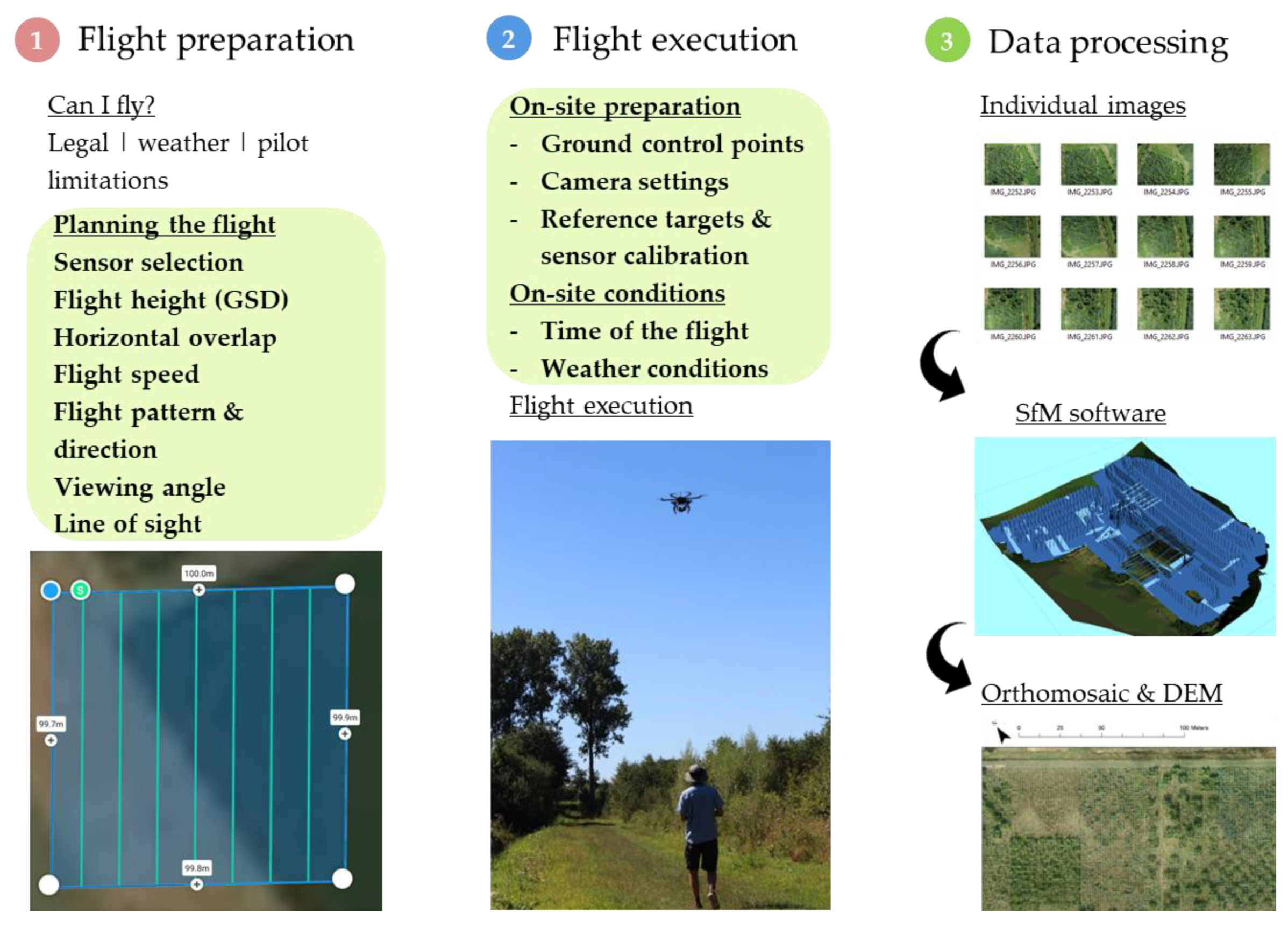
Figure 2.
Schematic overview of the solar and sensor viewing angles.
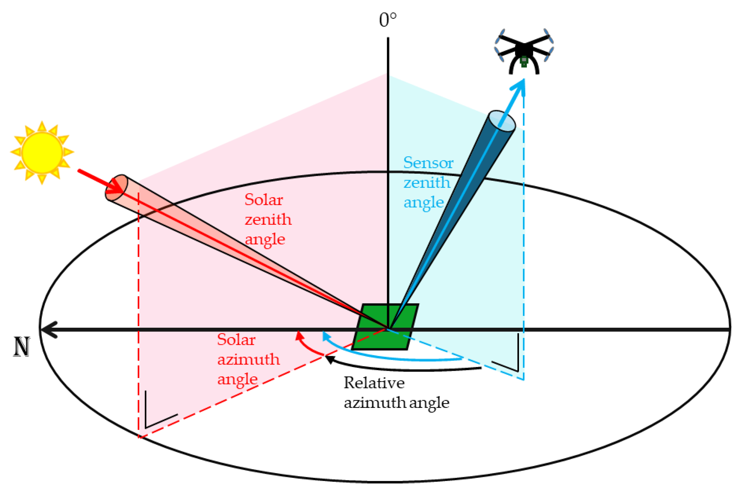
Figure 3.
BRDF influence on spectral reflectance. a) Images obtained with a drone from a meadow from different sensor zenith and azimuth angles (Canon S110 camera, on a Vulcan hexacopter with an AV200 gimbal (PhotoHigher, Wellington, New Zealand), obtained on 28 July 2015 over a meadow near Richmond, NSW, Australia (lat: 33.611°S, lon: 150.732°E). b) empirical BRDF in the Green wavelength over a tropical forest (Robson Creek, Queensland, Australia (lat: -17.118S, lon:145.630), obtained with the same UAV and camera, obtained on 16 August 2015, from [19], c, d & e: simulations of reflectance in the red (c) and near infrared (d) spectrum and for the NDVI (e) (SCOPE; for a vegetation of 1m height, LAI of 2, Chlorophyll content of 40 μg/cm² and fixed solar zenith angle of 30°).
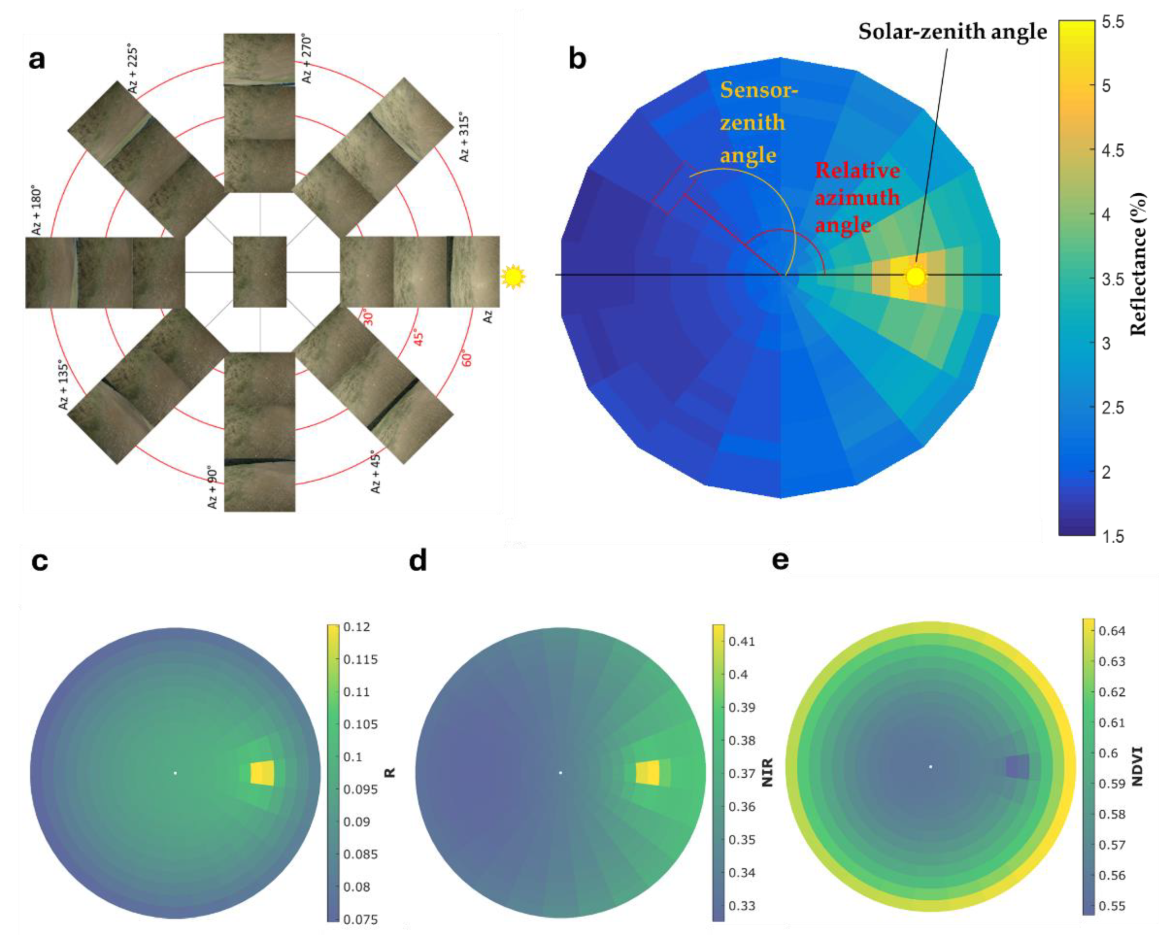
Figure 5.
The effect of ground sampling distance on the image quality, in this case for weed detection in a corn field. Image taken on 14/07/2022 in Bottelare, Belgium, with a Sony α4mIII camera, equipped with a 85 mm lens flying at 18m altitude. Here, a small section of the orthomosaic, created in Agisoft Metashape, is shown. The original GSD was 0.85mm, which was downscaled and exported at different GSD using Agisoft Metashape.
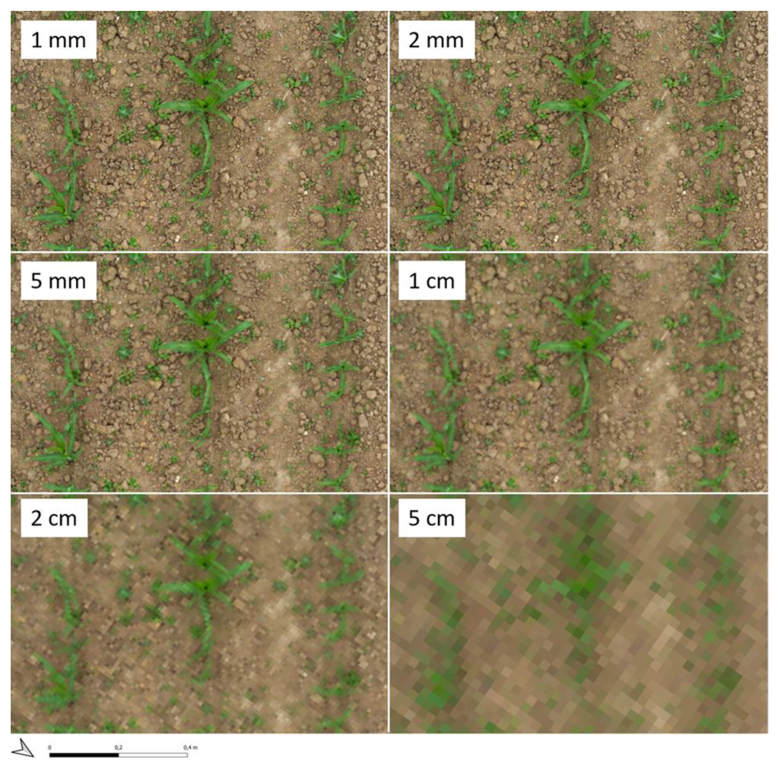
Figure 8.
The number of images collected for mapping a 1 ha (100m x 100m field -see Figure 6) with a Micasense RedEdge-MX multispectral camera as a function of the vertical and horizontal overlap. Image number was estimated in DJI Pilot.
Figure 8.
The number of images collected for mapping a 1 ha (100m x 100m field -see Figure 6) with a Micasense RedEdge-MX multispectral camera as a function of the vertical and horizontal overlap. Image number was estimated in DJI Pilot.
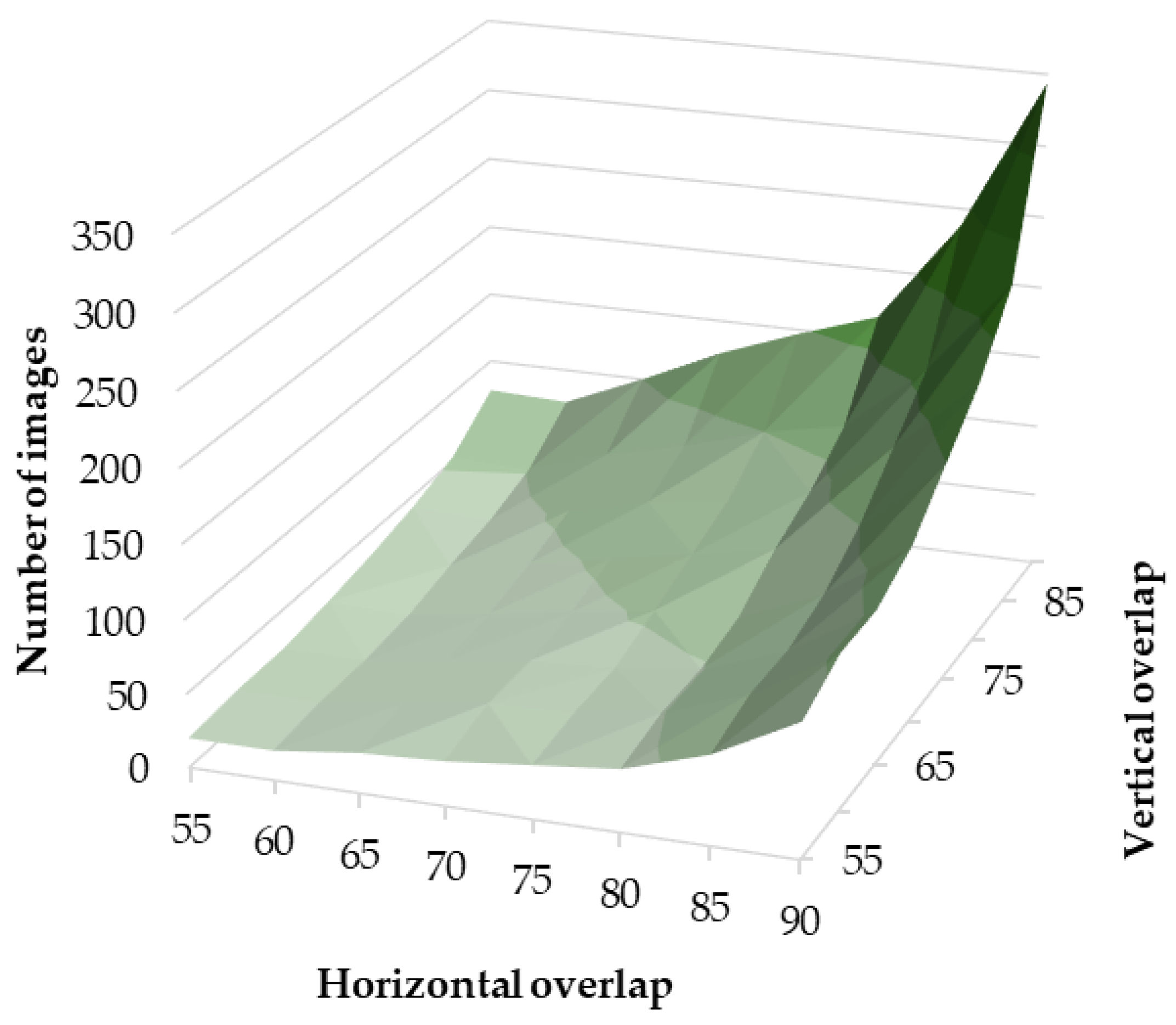
Figure 9.
Adjusted overlap (overlap needed to be given as input in the flight app) as a function of flight height and vegetation height, when the target overlap is 80%.
Figure 9.
Adjusted overlap (overlap needed to be given as input in the flight app) as a function of flight height and vegetation height, when the target overlap is 80%.
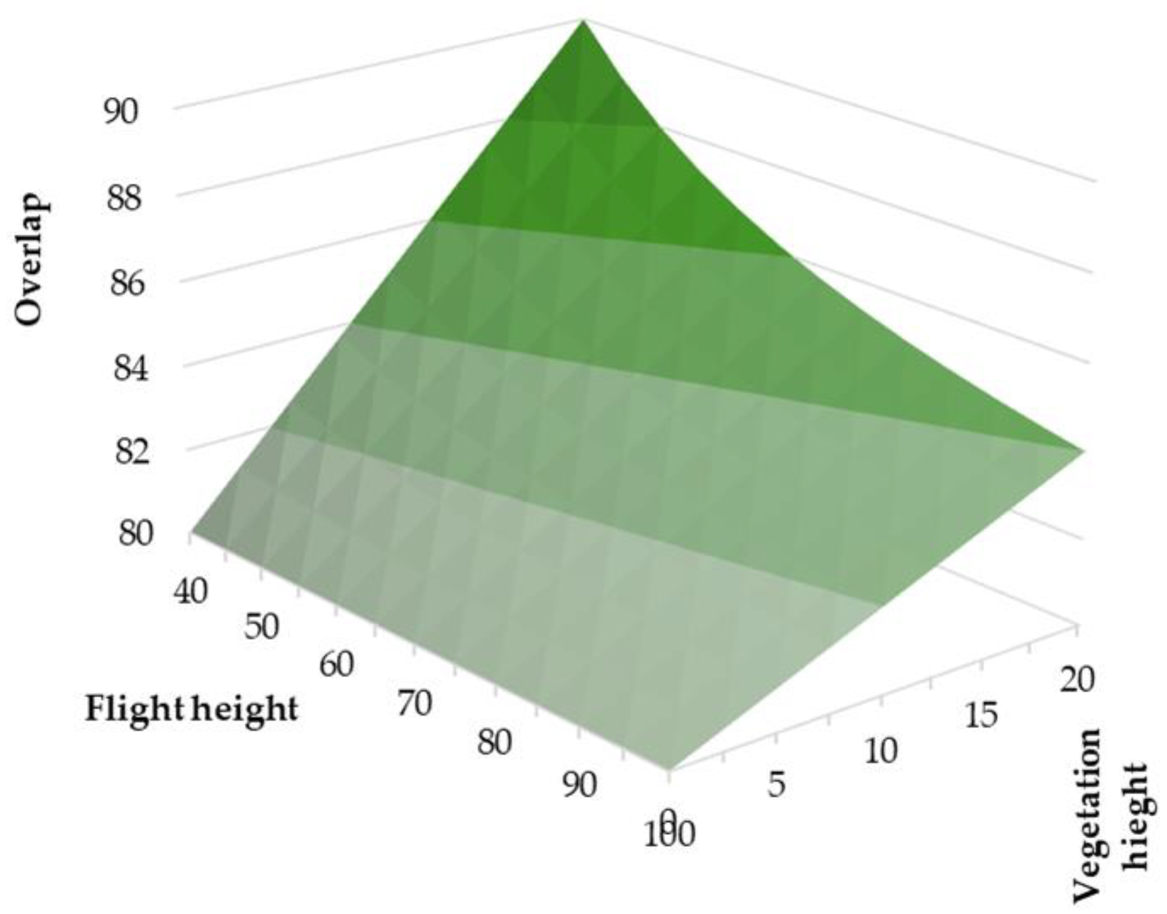

Table 1.
Summary of guidelines for flight planning for the different sensors.
| 3D model |
RGB (high resolution) |
Reflectance (multi-/ hyperspectral) |
Thermal | ||
| Terrain | Canopy | ||||
| Overlap | >70V, >50H | >80V, >70H* | >60V, >50H | >80V, >80H | >80V, >80H |
| Flight speed | Normal | Slow | Normal | Slow | |
| Pattern: grid? | Yes | No | No | No | |
| Flight direction | Standard | Standard | Perpendicular to sun** | Standard (?) | |
| Viewing angle | Include oblique | Nadir | Nadir | Nadir | |
* Additional corrections needed; can be higher (90%) when soil pixels should be included; ** Depending on the incoming light sensor; extra attention needed for avoiding hot spot; Different for aquatic remote sensing.
Table 2.
Maximum distance (m) a multicopter UAV can be flown respecting the visual line of sight (VLOS) restrictions according to two different approaches.
Table 2.
Maximum distance (m) a multicopter UAV can be flown respecting the visual line of sight (VLOS) restrictions according to two different approaches.
| Height (m) | Diagonal size (m) | Maximum distance (Eq. 5) | Maximum distance (Eq. 6) | |
| DJI Mini4 | 0.064 | 0.213 | 56 | 90 |
| DJI Mavic 3 | 0.107 | 0.381 | 94 | 145 |
| DJI Phantom | 0.28 | 0.59 | 245 | 213 |
| DJI M350 | 0.43 | 0.895 | 379 | 313 |
| DJI M600 | 0.759 | 1.669 | 669 | 566 |
Table 3.
Overview of the different factors needed to take into account when executing flights.
| 3D model | RGB | Reflectance | Thermal | ||
| Terrain | Canopy | (high resolution) | (multi-/hyperspectral) | ||
| Sunny conditions? | Not required | Less relevant | Preferable, but not required | Required | |
| Wind speed? | Not relevant | Low | Best low, but can be higher | Best low, but can be higher | Low |
| Time of flight | Not relevant | Less relevant | Solar noon (but avoid hot spot) | Solar noon (but avoid hot spot) | |
| GCP | Yes | Yes | Yes | Yes | |
| Reference targets | Not relevant | Grey panels recommended | Single or (better) multiple grey panels | Aluminium foil-covered panel + temperature panels (+ extreme temperature panels) | |
Disclaimer/Publisher’s Note: The statements, opinions and data contained in all publications are solely those of the individual author(s) and contributor(s) and not of MDPI and/or the editor(s). MDPI and/or the editor(s) disclaim responsibility for any injury to people or property resulting from any ideas, methods, instructions or products referred to in the content. |
© 2024 by the authors. Licensee MDPI, Basel, Switzerland. This article is an open access article distributed under the terms and conditions of the Creative Commons Attribution (CC BY) license (http://creativecommons.org/licenses/by/4.0/).
Copyright: This open access article is published under a Creative Commons CC BY 4.0 license, which permit the free download, distribution, and reuse, provided that the author and preprint are cited in any reuse.


