Submitted:
28 November 2024
Posted:
30 November 2024
You are already at the latest version
Abstract
Finite difference methods are commonly used in the pricing of discretely monitored exotic options in the Black-Scholes framework, but they tend to converge slowly due to discontinuities contained in terminal conditions. We present an effective analytical modification to existing finite difference methods which greatly enhances their performance on discretely monitored options with non-smooth terminal conditions. We apply this modification to the popular Crank-Nicolson method and obtain highly accurate option pricing results with significantly reduced CPU cost. We also introduce an adaptive mesh refinement technique which further improves the computational speed of the modified finite difference method. The proposed method is especially useful for options with high monitoring frequencies, which are difficult to price using other existing methods.
Keywords:
Discrete option pricing
; finite difference method
; analytical modification
; autocallable structured product
; barrier option
; snowball option
1. Introduction
Discretely monitored exotic options, including barrier options and autocallable structured products, are commonly traded throughout the world. Unlike continuously monitored barrier options, discrete barrier options cannot be priced using analytical formulas. Instead, these options are priced using numerical techniques such as Monte-Carlo simulations, finite difference methods, quadrature methods [1,2], and several other sophisticated mathematical techniques (e.g. [3,4,5,6,7]). Discrete barrier options can also be priced approximately using continuity correction techniques [8,9], but the accuracy of these methods is often quite limited.
To price options with low to moderate monitoring frequencies (e.g. monthly), quadrature methods can be quite effective [2]. However, these methods are not suitable for pricing options with high monitoring frequencies (e.g. daily), since they involve computations of convolution integrals at all monitoring points (or barriers), which can be very expensive when monitoring frequencies become large. Monte-Carlo simulations suffer from the same limitation, where significantly more random numbers need to be generated along a rapidly increasing number of paths as monitoring frequencies increase. Finite difference methods, in contrast, are not subject to such limitations, as long as monitoring points are placed on the computational grid, but they tend to converge slowly due to discontinuities contained in terminal conditions. Performance of finite difference methods can be improved using advanced numerical techniques such as adaptive mesh models [10], Rannacher time-stepping [11,12], and the TR-BDF2 method [13], but these methods either are formulated in a different setting (e.g. for tree-based pricing models [10]), or suffer from relatively low accuracies due to the incorporation of low-order approximations near terminal/boundary points (e.g. [11,12]).
We present an analytical modification to finite difference methods in the Black-Scholes framework to remove any discontinuities contained in the terminal conditions, which greatly improves the accuracy and efficiency of these methods. We will apply the modification to the popular Crank-Nicolson method, and introduce an effective adaptive mesh refinement technique to further improve the computational speed of the modified method. The modified finite difference method is valuable in practice thanks to its high accuracy and ease of implementation. It also complements our previous quadrature method [2] since its performance is unaffected by higher monitoring frequencies.
1.1. A Brief Review of Products Considered
The modified finite difference method is applicable to various types of discretely monitored options, including discrete barrier options, autocallable structured products, and snowball options.
Barrier options are among the most popular types of exotic options. A barrier option may be activated (knock-in option) or deactivated (knock-out option) when the underlying asset price crosses certain barrier levels. A single barrier option has one barrier at each observation date, while a double barrier option has two barriers at each observation date. The final payoff of a barrier option (if it is active at maturity) may be of the same type as that of a vanilla option or that of a digital option.
For an autocallable product, there is a pre-specified barrier level at each observation date. If the underlying asset price is greater (less) than or equal to the barrier level, the option is exercised and a pre-specified fixed-rate return is paid. If the asset price is below (above) the barriers at all observation dates, the option is never exercised and the investor receives a negative return at maturity.
A snowball option has an up-and-out barrier and a down-and-in barrier, and the down-and-in barrier is usually monitored daily. If the asset price reaches the up-and-out barrier, the option is exercised and a pre-specified fixed-rate return is paid. If the option expires without any barrier being reached, the investor receives a fixed coupon payment. If the up-and-out barrier is never reached but the down-and-in barrier is reached sometime before maturity, the investor automatically writes a vanilla put and may receive a negative return.
1.2. Organization of the Paper
The rest of the paper is organized as follows. Section 2.1 defines the class of (discrete) option pricing problems that our method is intended to solve, and the rest of Section 2 details the various ingredients of our method including, specifically, the analytical modification (Section 2.3) we introduce for standard finite difference methods (Section 2.2) in the context of discrete option pricing, and an adaptive mesh refinement technique for the analytically modified finite difference methods (Section 2.4). The efficacy and efficiency of our method is then demonstrated through extensive numerical studies in Section 3, and the paper is concluded in Section 4.
2. Materials and Methods
2.1. Basic Assumptions
We consider a general class of discretely monitored options with barriers. Note that an option with knock-in barriers is equivalent to the difference of an option without those knock-in barriers and another option with knock-out barriers at the same dates and same levels. Therefore, it suffices to consider options with only knock-out barriers. To this end, assume that
- (A)
- The option to be priced has two strike prices , with , at each observation date . The expiration date is .
- (B)
- The option is exercised if or at some , and the payoffs are given by (if ) and (if ), respectively, for some .
- (C)
- The final payoff at maturity isfor some .
These assumptions are general enough to cover a wide class of discretely monitored options, such as the ones mentioned in the introduction. For instance, down-and-out put barrier options would have
Double barrier knock-out call options would have
Common up-and-out autocallable products would have
We further assume that the price of the underlying asset satisfies the following stochastic differential equation under the risk-neutral measure:
where is the risk-free forward interest rate, the yield rate, the volatility, and the Wiener process. Interest rates, yield rates, and volatilities are assumed to be deterministic functions of time.
To summarize, our basic assumptions are
- There are finitely many observation points, and two exercise levels (possibly ∞) at each observation point. If S is above the upper exercise level or below the lower exercise level at any observation point, the option is exercised and the payoff is a linear function in S.
- At maturity, if S is between the two exercise levels, a payoff is incurred which is also a linear function in S.
- The underlying asset price S follows a geometric Brownian motion with possibly time-dependent interest rates, yield rates, and volatilities.
Given the above assumptions, we shall begin the description of our method with a brief review of the finite difference methods commonly used in the pricing of discretely monitored options.
2.2. Finite Difference Methods
Suppose we wish to find an option’s value at some and the spot price of the underlying asset is . Let denote the value of the option (as a function of the asset price S) at any time . Since S follows a geometric Brownian motion, the option’s value satisfies the Black-Scholes PDE
for , with the terminal condition
and boundary conditions
determined by Assumptions (B)–(C) from Section 2.1.
For convenience, we introduce the change of variable to transform equation (2.2a) into a simpler form:
where the differential operator is defined as
It is not convenient to solve the PDE (2.3a) directly due to the discrete boundary conditions (2.2c). Instead, for each , we consider the PDE
supplemented with the terminal condition
Since the terminal value problem (2.4) has a unique solution for each m, we have
and by (2.2c),
The terminal value problems (2.4) are solved successively for . Note that for , the terminal condition is known by (2.2b). Now for each , assume the terminal condition is known. The PDE (2.4a) is solved backward in t to yield . Then we obtain by (2.5), which by (2.4b) is equal to , the terminal condition of the PDE (2.4a) for . This process can then be repeated until we finally obtain , from which the option’s value can be easily deduced.
Now we give a brief review of the standard procedure of solving (2.4) numerically on a uniform grid using finite difference methods. Let denote the grid points in time, and the grid points in space where . Denote
In practice, barriers are observed at the end of a business day, so it is convenient to find a uniform t-grid such that every monitoring point lies on the grid, i.e. for every , there exists an such that . The PDE (2.4a) can be discretized using the backward-time centered-space (BTCS), forward-time centered-space (FTCS), or Crank-Nicolson (C-N) finite difference method.
The BTCS (or explicit Euler) method consists of the recurrence equations
and is explicit (recall that we are solving (2.4a) backward in time). The FTCS (or implicit Euler) method, on the other hand, consists of the recurrence equations
and is implicit. The C-N method is a combination of the BTCS and FTCS methods and can be written as
For , we impose the extrapolation boundary condition1
which is equivalent to
and can be discretized as
The C-N method is generally more accurate than the BTCS and FTCS methods [14], although the FTCS method has better stability properties [13].
For convenience, we denote
Equations (2.8) and (2.9c) can be written together as a matrix equation
where
is a -column vector and are tridiagonal matrices:
where
Note that the unknowns in the equation and in the equation for can be eliminated using the boundary condition (2.9c). Equation (2.10a) can be solved for using the Thomas Algorithm, which has an complexity.
Note that the terminal condition (2.4b) is typically discontinuous as can be seen from (2.5). This means that the C-N method, when applied as it is, cannot achieve a second-order convergence as for smooth terminal conditions [11].
2.3. Analytical Modification
We will remove the aforementioned discontinuities from terminal conditions by introducing an analytical modification to existing finite difference methods. First, we recall some classical results from the theory of binary options.
Lemma 2.1.
Let , and let denote the characteristic function of a set A. Consider a binary option with expiration time priced at .
- 1.
- If the option has payoff , then .
- 2.
- If , then .
- 3.
- If , then .
- 4.
- If , then .
The functions and are defined as
where ,
is the cumulative normal distribution function, and
Proof.
By definition, is the value of an asset-or-nothing option, and is the value of a cash-or-nothing option. The valuation formulas are just standard results for binary options [14]. □
Since in the terminal condition (2.4b) generally has discontinuities at , we do not solve the terminal value problem (2.4) directly, but instead seek to remove these discontinuities first. We describe our basic idea as follows.
2.3.1. Basic idea of the analytical modification
For each , note that is continuous for . We define the one-sided limits
and consider defined as the solution to the PDE
supplemented with the (continuously differentiable) terminal condition
Note that by (2.2b)-(2.2c), we have
where
This shows that is the sum of values of four binary options for , and hence by Lemma 2.1,
or
For each , we solve (2.12) numerically for and obtain using (2.14b). Repeating this process for , we finally obtain , from which the option’s value can be easily deduced.
Remark 2.2.
For the given terminal condition (2.2b), a closed-form expression can in fact be obtained for ; see, for example, [2]. In practice, however, M is often “reasonably large”, e.g., in the order of tens or hundreds, so that the incorporation of such exact formulas of makes little difference in the numerical approximations obtained for . Thus we do not specifically differentiate from other ’s () in our study.
2.3.2. Implementation of the Analytical Modification
In practice, it may not be possible to place all barriers on the computational grid, which means we may not be able to compute the values of for all as defined in (2.11). Note that the values of for follow from the closed-form expression of as given in (2.2b). For , however, we will have to find an approximation to these values. To this end, denote
which is the smooth solution defined in (2.12) for . For each , assume we have already computed a three times continuously differentiable () function for and have obtained the smooth part of , namely (see (2.5)), at the grid points. Note that this is true for , in which case we have already computed a function by (2.15) and have obtained by (2.14b).
Denote
and let
Note that are located between and . We use linear interpolations of on the grid to approximate as follows:
Since and hence is in Z, we have
This means that the order of the interpolation error does not exceed that of the C-N method.
Consider defined as the solution to the PDE
supplemented with the terminal condition
Note that by (2.2c), we have
where
This shows that is the sum of values of four binary options for , and hence by Lemma 2.1,
or
Now that we have computed and the smooth part of , namely , we continue to compute as in (2.16), which means we have the terminal condition as in (2.18b). Then we repeat this process for .
We summarize the modified finite difference method as follows:
- 1:
- for downto 1 do
- 2:
- Compute using (2.16)
- 3:
- Solve (2.18) numerically for
- 4:
- Compute , the smooth part of , using (2.20b)
- 5:
- end for
- 6:
- Obtain option value
Note that the terminal value problem (2.18) is the same as (2.4) except that the terminal condition (2.18b) now has a higher degree of smoothness, and the problem (2.18) can be solved numerically using the same finite difference methods as the ones described in Section 2.2, in particular the C-N method. Since the terminal condition in (2.18b) is almost continuously differentiable (the jumps are of order by (2.17)), the C-N method converges quite well in practice (Section 3.1). In principle, Rannacher time-stepping can be used to improve the performance of the C-N method near monitoring points, but this is important only when accurate discrete approximations to option Greeks are needed (Section 3.4).
2.4. Adaptive Mesh Refinement
Note that the function in (2.18) tends to have large derivatives near the barriers and behaves relatively smoothly away from the barriers. This means that it makes sense to use finer grids near the barriers and coarser ones elsewhere.
Adaptive mesh refinement techniques are well-known and are widely used in numerical solutions of PDEs. In the field of quantitative finance, adaptive mesh models have been developed for the BTCS method [10]. Alternatively, nonuniform grids based on changes of variables have also been introduced in the literature [13]. Since here we are using an analytically modified C-N method, we introduce an effective adaptive mesh refinement technique which further improves the computational efficiency of our method.
We begin by assuming that the upper barriers (and lower barriers , respectively) are equal or close to each other for all , which is almost always satisfied in practice. Our basic idea is to construct fine grids near the barriers, and solve the Black-Scholes PDEs on both the original and the fine grids at each time step.
First, we find integers such that
for all . Then we construct a fine grid for and a similar one for by dividing each interval of size h into n equal parts. We illustrate the fine grid near for in Figure 1.
Let
and define
which is the smooth solution defined in (2.12) for . For each , assume we have already computed a function for
and have obtained the smooth part of , namely , at the grid points. Note that this is true for by (2.21) and (2.14b).
Recall from (2.16) that are approximations to computed using the values of on the original (coarse) grid. We shall now find approximations to using the values of on the fine grids. To this end, denote
and let
Define
Note that, in general, provide a better approximation to than .
Consider defined as the solution to the PDE
supplemented with the terminal condition
The PDE (2.23a) is the same as (2.18a), but we do not solve it all the way back to . Instead, for each , assume we have computed for , which is true for by (2.23b). We first solve the PDE (2.23a) numerically using the terminal condition on the coarse grid for just one time step from to . More specifically, denote by the solution computed on the coarse grid; we solve the matrix equation (2.10a) which in our new notation becomes
where
is a -column vector and are tridiagonal matrices as defined in (2.10). After solving for from (2.24), we solve the PDE (2.23a) again on the fine grids for n time steps with reduced step size , using the boundary conditions linearly interpolated (in time) from at and . For convenience, we denote, for ,
and . The matrix equation on the fine grids then becomes
where
are -column vectors and are tridiagonal Toeplitz matrices:
Note that, in (2.25b),
are boundary conditions linearly interpolated (in time) from coarse grid solutions at and . After solving for from (2.25a), we set
and
Since for , equation (2.27) completes the definition of for . We then repeat this process for to obtain for .
By (2.23b), is piecewise linear in , meaning is the sum of values of four binary options. It follows from Lemma 2.1 that
where
Then we repeat this process for .
We summarize the adaptive mesh refinement procedure as follows:
- 1:
- Construct a fine grid for and a similar one for by dividing each interval of size h into n equal parts
- 2:
- for downto 1 do
- 3:
- Compute using (2.22)
- 4:
- Solve (2.23) numerically for one time step (with step size k) on coarse grid
- 5:
- Solve (2.23) numerically for n time steps (with step size ) on fine grids, using (2.26) as boundary conditions
- 6:
- Combine numerical solutions on coarse and fine grids to obtain
- 7:
- Compute , the smooth part of , using (2.28)
- 8:
- end for
- 9:
- Obtain option value
3. Results
3.1. Convergence Study
To study the convergence properties of the proposed method, either with or without mesh adaptation, we first apply the original and the analytically modified C-N method to the following five options:
- Option I: A cash-or-nothing call option with final payoff:
- Option II: An asset-or-nothing call option with final payoff:
- Option III: A vanilla call option with final payoff:
-
Option IV: An exotic call option with final payoff:We remark that this option does not have a counterpart in real-life financial applications. It is designed here solely to test the convergence properties of the proposed method.
These four options are standard options without discretely monitored structures, and for all cases we set
Note also that the final payoffs of the above four options have increasingly higher degree of smoothness (discontinuous, discontinuous, , and , respectively). The fifth option, on the other hand, is a discretely monitored option:
- Option V: A double-barrier knock-out option with different monitoring frequencies for the two barriers. Assume there are 250 business days in a year, and the option will expire one year from the valuation date which we denote as day 0. The spot price of the underlying asset at day 0 is 1.1. The upper barrier level is 1.2, and its observation dates are {15, 36, 57, 78, 99, 120, 141, 162, 183, 204, 225, 246}, resembling a monthly monitoring structure. The lower barrier is monitored daily, and the barrier level is 0.9. We further assume that the notional value of the option is 100, that the payoff at maturity is 10% of the notional value, namely 10, and that
In practice, this type of barrier structure is common for snowball options and their variants. Note that the lower barrier of a snowball option is a knock-in barrier, but the option can be priced as the difference between an up-and-out barrier option and a double-barrier knock-out option using PDE methods. Table 1, Table 2, Table 3, Table 4, Table 5, Table 6, Table 7 and Table 8 present results from convergence studies of the four standard options (I-IV) priced using the original C-N method. Since our purpose here is to examine numerically the relationship between convergence rates and smoothness of terminal conditions, the analytically modified C-N method is not used which otherwise would produce (almost) exact pricing results for the first three options (I-III). All four options are priced on the interval2
with a time step and a mesh size , where N ranges from 10 to 5,120. For the first three options, exact option values are available from analytical formulas, while for the fourth option, the option value is estimated on a finer grid with . For each numerical approximation to calculated at on the computational grid, two types of errors are defined:
The numerical order of an error ( or ) calculated on a grid of size N is estimated using the formula:
It can be observed from these tables that:
- For the first two options (I-II), the C-N method converges at only first order due to the discontinuity at contained in the terminal conditions. On the other hand, mesh adaptation around the discontinuity , where option prices are expected to undergo the most rapid variation, helps reduce the error by a factor of n where here is the refinement factor.
- For the next two options (III-IV), the C-N method converges at a higher order due to the improved smoothness of the terminal condition at . The precise relationship between the convergence rate and the smoothness of the terminal condition is the subject of a future research, but these examples seem to suggest that a terminal condition is already sufficient to restore the second-order accuracy of the C-N method (see Remark 3.2).
- When mesh adaptation is applied to the third option, the error first improves by roughly a factor of up until , after which no significant improvement in error is observed (Table 6). This is due to the fact that the terminal condition in this case has a higher degree of smoothness at (i.e., ), as a result of which the largest error on a sufficiently fine grid does not concentrate around , and hence is not captured by the adaptive mesh which surrounds the strike price . Similar observations apply to the fourth option, whose terminal condition has an even higher degree of smoothness at (i.e., ) and for which no improvement in error is observed for the adaptive mesh calculation at all.
- Despite these observations, the mesh adaptation technique still turns out to be useful when applied to discretely monitored options with high monitoring frequencies, where errors near the barriers caused by the non-smoothness of the terminal conditions dominate the calculations (Section 3.1, Section 3.3).
Remark 3.1.
Since the terminal conditions for the first two options contain a discontinuity at and since the C-N method, with or without analytical modifications, is non-dissipative, the following modification is needed in discrete approximations to so that the convergence of to in a suitable weak sense (e.g., in the sense of for some ), and hence the convergence of to , can be ensured: let be chosen such that
or equivalently, such that
Then for the first option, we set
and for the second option, we set
For the next two options, the terminal conditions are continuous throughout and hence such modification is not needed. One may simply take
For dissipative schemes such as FTCS and TR-BDF2, the above modification is not needed either.
Remark 3.2.
We have carried out a preliminary error analysis for the proposed method and found that the convergence rate corresponding to a discontinuous, , and terminal condition is , and , respectively. However, these results are likely suboptimal because they didn’t make full use of the dissipation properties of the Black-Scholes PDE.
Table 9, Table 10, Table 11, Table 12, Table 13 and Table 14 present results from convergence studies of the discretely monitored option (V) priced using both the original and the analytically modified C-N methods. To examine more closely the relationship between the convergence rate and the smoothness of the terminal conditions, we further distinguish between the following two cases for the analytically modified C-N method:
- A -modification at the barriers:which is (2.12b) with and which is only continuous at the barriers.
- A -modification at the barriers:which is just (2.12b) and is continuously differentiable at the barriers.
For all three methods, namely, original C-N and analytically modified C-N with - and -modifications, the option is priced on the same interval as in the previous cases:
The calculations are advanced with a time step , i.e., with time steps per business day, and with a mesh size where ranges from 1 to 64. Since the exact option values are not available, reference values against which all numerical approximations are compared are calculated on a uniform fine grid using the analytically modified C-N method with a -modification at the barriers and with time steps per business day.
It can be observed from these tables that:
- For the original C-N method, the numerical approximations converge to the reference values in at an average rate of roughly 1 but do not converge in at all (Table 9). This reduced convergence rate or even lack of convergence is clearly a consequence of the discontinuities at the barriers contained in the terminal conditions. On the other hand, mesh adaptation around the barriers, where option prices are expected to undergo the most rapid variation, helps reduce the error by a factor of n where here is the refinement factor (Table 10).
- For the analytically modified C-N method, with either - or -modifications, the numerical approximations converge to the reference values in both and and do so at a higher rate due to the improved smoothness of the terminal conditions at the barriers. More specifically, with -modifications, converge to in at an average rate of roughly and in at an average rate of roughly 1 (Table 11), while with -modifications, the convergence in both and has an average rate of roughly 2 (Table 13). In other words, these examples seem to suggest that a -modification to the terminal conditions is already sufficient to restore the second-order accuracy of the C-N method.
- When mesh adaptation is applied with -modifications, both the - and -errors improve by roughly a factor of for all , demonstrating the effectiveness of the adaptive mesh (Table 12).
- When mesh adaptation is applied with -modifications, the numerical approximations calculated on the finest grid with are almost identical with the reference values calculated on the uniform fine grid with , as suggested by the unusually small errors (last row, Table 14). On the other hand, for numerical approximations calculated on coarser grids with , both the - and -errors improve by roughly a factor of for all when mesh adaptation is enabled. This provides another strong evidence for the effectiveness of the adaptive mesh, especially on discretely monitored options with high monitoring frequencies.
- We remark that for mesh adaptation applied with -modifications, a sufficiently large area around the barriers needs to be refined in order for the adaptive mesh to be effective, in view of the improved smoothness of the terminal conditions near the barriers. Indeed, when the refinement ratio in Table 14 was reduced from 15% to 10%, meaning only the grid points around each barrier are refined, the resulting adaptive mesh was only able to produce marginal improvement in error for and was not able to produce any meaningful improvement in error at all for all larger . This is not an issue when mesh adaptation is applied with -modifications or with no analytical modifications, where the errors near the barriers caused by the non-smoothness of the terminal conditions dominate the calculations.
3.2. Comparison with other Numerical Methods
To assess the efficacy and efficiency of the proposed method on options with discretely monitored structures, we next apply other popular, (formally) second-order numerical methods such as C-N with Rannacher time-stepping (CN-RAN) and trapezoidal rule with second-order backward differentiation formula (TR-BDF2) to the discretely monitored option introduced in the previous section. Both methods (CN-RAN and TR-BDF2) have been applied to the four standard options introduced above, and their convergence properties have been found to be very similar to those of the original C-N method (Table 1, Table 3, Table 5 and Table 7).
Table 15 and Table 16 present results from convergence studies of the discretely monitored option priced using the CN-RAN and the TR-BDF2 methods. It can be observed from these tables that:
- Both methods exhibit very similar convergence behaviors and converge in both and at an average rate of roughly 1. This shows, in particular, that both methods lose their second-order accuracy when applied to problems containing discontinuities.
As a more direct comparison of the different numerical methods studied in the literature (including in this work) and commonly used in practice, we list in Table 17 the pricing results of the following five methods applied to the discretely monitored option introduced in the previous section:
- Analytically modified C-N with a -modification (CN-C1).
- C-N with Rannacher time-stepping (CN-RAN).
- Trapezoidal rule with second-order backward differentiation formula (TR-BDF2).
- Forward-time centered-space (or implicit Euler) (FTCS).
- Monte-Carlo simulations (MC).

Table 17.
Comparison of different methods on a discretely monitored option.
| Time Steps | CN-C1 | CN-RAN | ||
| CPU time | CPU time | |||
| 1 | ||||
| 2 | ||||
| 4 | ||||
| 8 | ||||
| 16 | ||||
| 32 | ||||
| 64 | ||||
| Reference option value at : 1.83652751. | ||||
| TR-BDF2 | FTCS | |||
| CPU time | CPU time | |||
| 1 | ||||
| 2 | ||||
| 4 | ||||
| 8 | ||||
| 16 | ||||
| 32 | ||||
| 64 | ||||
| Reference option value at : 1.83652751. | ||||
| Number | MC | |||
| 40000 | ||||
| 60000 | ||||
| 80000 | ||||
| 100000 | ||||
| 120000 | ||||
| 140000 | ||||
| 160000 | ||||
| Reference option value at : 1.83652751. | ||||
For each method, the (pointwise) error of the option value at , together with the CPU time (in seconds)3 used to obtain the pricing result, are shown for different time steps . Each CPU time is measured by running the corresponding code 5 times and dividing the total CPU time by 5. It can be observed from the table that for a given level of accuracy, the CN-C1 method requires the least amount of CPU time while all other four methods typically require significantly more CPU time. As a specific example, consider the accuracy level of . A more refined study shows that to achieve this level of accuracy, the CN-C1 method requires less than 0.5618 seconds while the other four methods require
- 16.7132 seconds (CN-RAN),
- 36.1549 seconds (TR-BDF2),
- 22.8074 seconds (FTCS), and
- 26.4529 seconds (MC),
respectively (Table 18). This confirms the efficiency of the CN-C1 method.
Table 18.
CPU time (in seconds) required to achieve an accuracy level of by different methods on a discretely monitored option.
Table 18.
CPU time (in seconds) required to achieve an accuracy level of by different methods on a discretely monitored option.
| Time Steps | CN-C1 | Time Steps | CN-RAN | ||
| 1 | 43 | ||||
| − | − | − | 44 | ||
| − | − | − | |||
| Reference option value at : 1.83652751. | |||||
| *: Estimates obtained from linear interpolation. | |||||
| TR-BDF2 | FTCS | ||||
| 42 | 65 | ||||
| 43 | 66 | ||||
| Reference option value at : 1.83652751. | |||||
| *: Estimates obtained from linear interpolation. | |||||
| Number | MC | ||||
| 108300 | |||||
| 108400 | |||||
| Reference option value at : 1.83652751. | |||||
| *: Estimates obtained from linear interpolation. | |||||
Remark 3.3.
It may appear from these results that MC is even more efficient that the TR-BDF2 method. The reality is that, if higher accuracy is demanded (higher than ), then the TR-BDF2 method will definitely outperform MC, even though it is relatively slow compared with other finite difference methods considered here.
3.3. Effectiveness of Adaptive Mesh Refinement
We also demonstrate the effectiveness of the mesh adaptation technique by applying the CN-C1 method to the discretely monitored option introduced in the previous sections, both with and without mesh adaptation. The result shows that, with a mesh refinement factor of , an adaptive mesh calculation with time steps per business day is able to achieve an accuracy level comparable to that of a uniform grid calculation with time steps per business day, with a more than 60% save in CPU time (Table 19). This confirms the efficiency of the mesh adaptation technique.
3.4. Approximations to Derivatives
It is well known that finite difference methods applied to options with non-smooth terminal conditions tend to produce poor approximations to option Greeks such as Delta and Gamma . In fact, as demonstrated in [11], when the original C-N method is applied to a European call option, the discrete approximations to and both fail to converge, and the discrete approximation to even grows unboundedly when the computational grid is refined. To examine the quality of the discrete approximations to option Greeks produced by the proposed method, we calculate and for the discretely monitored option introduced in the previous section, using the formulas
where are the same reference option values calculated on a uniform fine grid using the CN-C1 method with time steps per business day. The approximated Greeks are shown in Figure 2 and Figure 3 together with the option values, where it can be seen that while the discrete approximation to is free of oscillations, the discrete approximation to contains a small amount of oscillations near the lower barrier 0.9 which is monitored daily. These oscillations are likely consequences of the errors introduced by the linear interpolation approximations to at the barriers (see (2.17)) which have been significantly amplified by the high-frequency monitoring at the lower barrier. To remove these high-wavenumber oscillations, we replace the first C-N step after each monitoring point by two half-step dissipative steps such as FTCS (implicit Euler) steps and apply the resulting method, coded CN-C1-RAN1, again to the discretely monitored option introduced in the previous section. The results (Figure 4) demonstrate the effectiveness of the modified method in the elimination of high-wavenumber oscillations and also confirm the second-order convergence of both the option value V and option Greeks in both and (Table 20).
Remark 3.4.
When applied with mesh adaptation, the CN-C1-RAN1 method produces option Greeks converging at reduced convergence rates, most likely due to the small mismatches among different parts of introduced by the direct transfer of the fine grid solutions to coarse grid (see (2.27)). While this issue may be addressed using, say, a high-order smoothing operator, we decide not to pursue this direction further but instead recommend the readers to consider CN-C1-RAN1 (without mesh adaptation) if accurate approximation to option Greeks is important and to consider CN-C1 (with or without mesh adaptation) if option Greeks are not needed or not important.
4. Discussion
We have introduced an analytical modification for finite difference methods used in the pricing of discretely monitored options in the Black-Scholes framework. The modified finite difference methods can be used to price single and double barrier options, autocallable structured products, and snowball options. We have demonstrated the efficacy and efficiency of the proposed method on the traditional Crank-Nicolson scheme which, in its analytically modified form CN-C1 or CN-C1-RAN1, is capable of producing much more accurate pricing results with much lower CPU cost than other popular option pricing methods such as CN-RAN, TR-BDF2, and Monte-Carlo simulations. We have also introduced a mesh adaptation technique for the analytically modified Crank-Nicolson method, which is capable of achieving an accuracy level comparable to that of a uniform fine grid calculation with a more than 60% improvement in computational speed. We strongly believe that the proposed method and the related ideas will prove a valuable tool for practitioners working with the aforementioned types of options.
This work can be extended in several directions. First, it is desirable to carry out a rigorous error analysis and obtain a precise quantification of the relationship between convergence rates and smoothness of terminal conditions for the proposed method. We have done some preliminary analysis along this direction (Remark 3.2) and the full analysis is currently a work in progress. Second, the proposed method has assumed a volatility that is independent of the asset price S, which may be too restrictive in some practical situations. It is desirable to relax this assumption and apply similar analytical modifications to option pricing problems with variable (in S) volatility. This is the subject of a current research and the results will be reported in a forthcoming paper.
Author Contributions
Conceptualization, M.H.; methodology, G.L. and M.H.; software, G.L. and M.H.; validation, G.L.; formal analysis, G.L.; investigation, G.L. and M.H.; writing—original draft preparation, G.L. and M.H.; writing—review and editing, G.L. All authors have read and agreed to the published version of the manuscript.
Funding
This research received no external funding.
Institutional Review Board Statement
Not applicable.
Informed Consent Statement
Not applicable.
Data Availability Statement
Data sharing is not applicable.
Conflicts of Interest
M.H. participated in this research as an independent individual. This work is not related in any way to his current employer, China Merchants Bank. The statements made and opinions expressed here in this paper are solely of the authors’ own. They do not reflect the views of China Merchants Bank or its employees and affiliates whatsoever. The authors declare no conflict of interest.
References
- A. Andricopoulos, M. A. Andricopoulos, M. Widdicks, P. Duck, D. Newton, Universal option valuation using quadrature methods, J. Financ. Econ. 67 (3) (2003) 447–471. [CrossRef]
- M. Huang, G. Luo, A simple and efficient numerical method for pricing discretely monitored early-exercise options, Appl. Math. Comput. 422 (2022) 126985. [CrossRef]
- G. Fusai, I. G. Fusai, I. Abrahams, C. Sgarra, An exact analytical solution for discrete barrier options, Finance Stochast. 10 (1) (2006) 1–26. [CrossRef]
- L. Feng, V. L. Feng, V. Linetsky, Pricing discretely monitored barrier options and defaultable bonds in Lévy process models: a fast Hilbert transform approach, Math. Financ. 18 (3) (2008) 337–384. [CrossRef]
- F. Fang, C.; F. Fang, C. Oosterlee. Pricing early-exercise and discrete barrier options by Fourier-cosine series expansions. Numer. Math. 2009, 114, 27–62. [Google Scholar] [CrossRef]
- L. Feng, X. L. Feng, X. Lin, Pricing Bermudan options in Lévy process models, SIAM J. Finan. Math. 4 (1) (2013) 474–493. [CrossRef]
- A. Golbabai, L. A. Golbabai, L. Ballestra, D. Ahmadian, A highly accurate finite element method to price discrete double barrier options, Comput. Econ. 44 (2) (2014) 153–173. [CrossRef]
- M. Broadie, P. M. Broadie, P. Glasserman, S. Kou, A continuity correction for discrete barrier options, Math. Financ. 7 (4) (1997) 325–348. [CrossRef]
- J. Wei, Valuation of discrete barrier options by interpolations, J. Deriv. 6 (1) (1998) 51–73. [CrossRef]
- D.-H. Ahn, S. D.-H. Ahn, S. Figlewski, B. Gao, Pricing discrete barrier options with an adaptive mesh model, J. Deriv. 6 (4) (1999) 33–43. [CrossRef]
- M. Giles, R. M. Giles, R. Carter, Convergence analysis of Crank-Nicolson and Rannacher time-marching, J. Comput. Financ. 9 (4) (2006) 89–112. [CrossRef]
- R. Rannacher, Finite element solution of diffusion problems with irregular data, Numer. Math. 43 (1984) 309–327. [CrossRef]
- F. Le Floc’h, TR-BDF2 for fast stable American option pricing, J. Comput. Financ. 17 (3) (2014) 31–56. [CrossRef]
- J. Hull, Options, Futures, and Other Derivatives, 9th Edition, Pearson, 2014.
| 1 | Note, in view of the linear boundary condition (2.2c), that the extrapolation boundary condition (2.9a) is a natural choice of the numerical boundary condition at . |
| 2 | Note that the actual computational domain is . |
| 3 | The code is developed in Python and is run on a personal computer. |
Figure 1.
Illustration of the original grid (solid lines) and the fine grid (dashed lines) near the barrier (thick line).
Figure 1.
Illustration of the original grid (solid lines) and the fine grid (dashed lines) near the barrier (thick line).
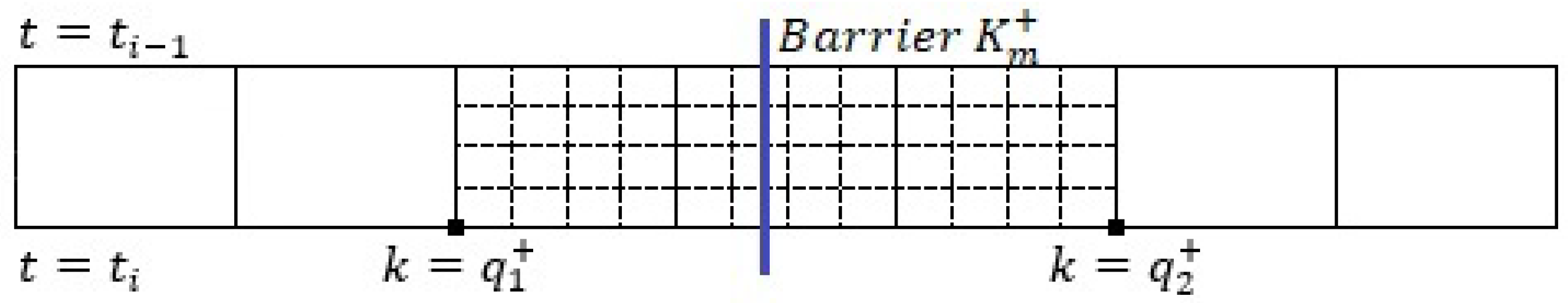
Figure 2.
Option values V (top) and Delta (bottom) estimated using the CN-C1 method on a uniform fine grid with time steps per day.
Figure 2.
Option values V (top) and Delta (bottom) estimated using the CN-C1 method on a uniform fine grid with time steps per day.
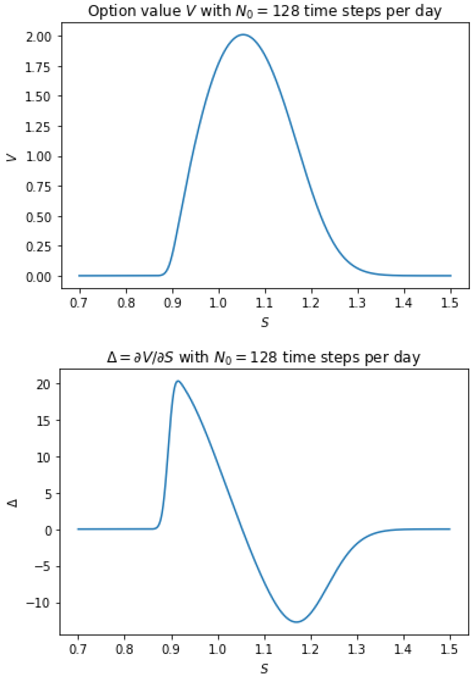
Figure 3.
Option Gamma (top) estimated using the CN-C1 method on a uniform fine grid with time steps per day and a closeup of the plot (bottom).
Figure 3.
Option Gamma (top) estimated using the CN-C1 method on a uniform fine grid with time steps per day and a closeup of the plot (bottom).
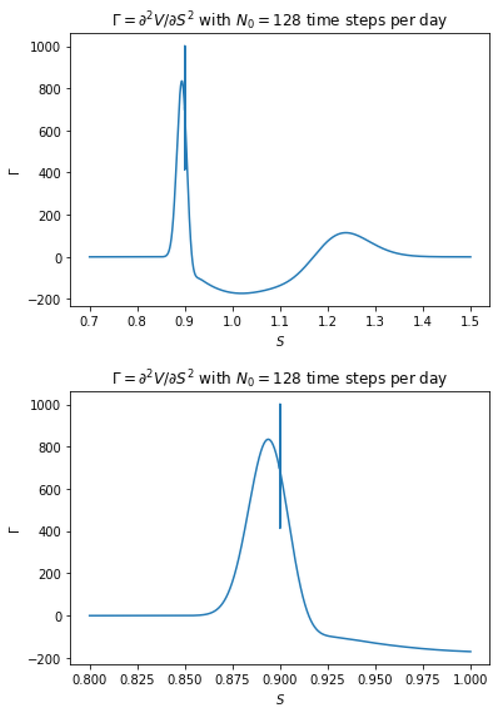
Figure 4.
Option Gamma (top) estimated using the CN-C1-RAN1 method on a uniform fine grid with time steps per day and a closeup of the plot (bottom).
Figure 4.
Option Gamma (top) estimated using the CN-C1-RAN1 method on a uniform fine grid with time steps per day and a closeup of the plot (bottom).
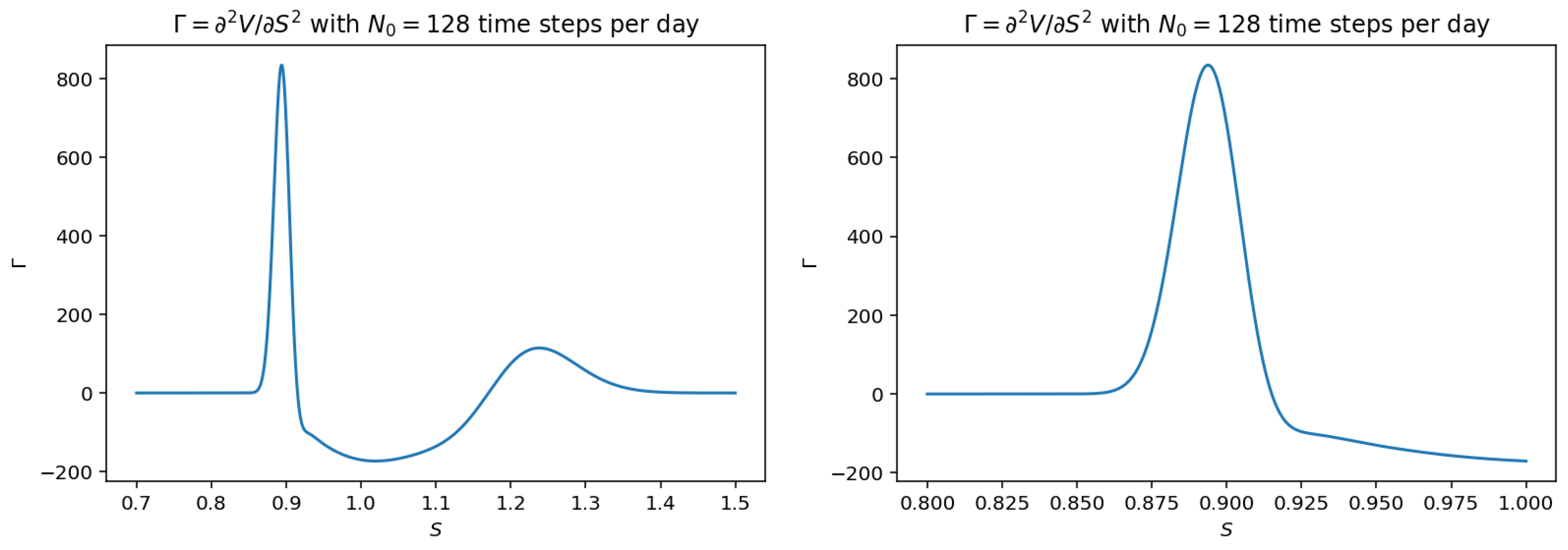
Table 1.
Unmodified C-N on a cash-or-nothing call option.
| -error | -error | |||
|---|---|---|---|---|
| 10 | − | − | ||
| 20 | ||||
| 40 | ||||
| 80 | ||||
| 160 | ||||
| 320 | ||||
| 640 | ||||
| 1280 | ||||
| 2560 | ||||
| 5120 | ||||
| Exact option value at : 32.5191. | ||||
Table 2.
Unmodified C-N with mesh adaptation (refinement region: grid points surrounding strike price; refinement ratio: 10% of grid points; refinement factor: 2) on a cash-or-nothing call option.
Table 2.
Unmodified C-N with mesh adaptation (refinement region: grid points surrounding strike price; refinement ratio: 10% of grid points; refinement factor: 2) on a cash-or-nothing call option.
| -error | -error | |||
|---|---|---|---|---|
| 10 | − | − | ||
| 20 | ||||
| 40 | ||||
| 80 | ||||
| 160 | ||||
| 320 | ||||
| 640 | ||||
| 1280 | ||||
| 2560 | ||||
| 5120 | ||||
| Exact option value at : 32.5191. | ||||
Table 3.
Unmodified C-N on an asset-or-nothing call option.
| -error | -error | |||
|---|---|---|---|---|
| 10 | − | − | ||
| 20 | ||||
| 40 | ||||
| 80 | ||||
| 160 | ||||
| 320 | ||||
| 640 | ||||
| 1280 | ||||
| 2560 | ||||
| 5120 | ||||
| Exact option value at : 44.7791. | ||||
Table 4.
Unmodified C-N with mesh adaptation (refinement region: grid points surrounding strike price; refinement ratio: 10% of grid points; refinement factor: 2) on an asset-or-nothing call option.
Table 4.
Unmodified C-N with mesh adaptation (refinement region: grid points surrounding strike price; refinement ratio: 10% of grid points; refinement factor: 2) on an asset-or-nothing call option.
| -error | -error | |||
|---|---|---|---|---|
| 10 | − | − | ||
| 20 | ||||
| 40 | ||||
| 80 | ||||
| 160 | ||||
| 320 | ||||
| 640 | ||||
| 1280 | ||||
| 2560 | ||||
| 5120 | ||||
| Exact option value at : 44.7791. | ||||
Table 5.
Unmodified C-N on a vanilla call option.
| 10 | − | − | ||
| 20 | ||||
| 40 | ||||
| 80 | ||||
| 160 | ||||
| 320 | ||||
| 640 | ||||
| 1280 | ||||
| 2560 | ||||
| 5120 | ||||
| Exact option value at : 5.75609968. | ||||
Table 6.
Unmodified C-N with mesh adaptation (refinement region: grid points surrounding strike price; refinement ratio: 10% of grid points; refinement factor: 2) on a vanilla call option.
Table 6.
Unmodified C-N with mesh adaptation (refinement region: grid points surrounding strike price; refinement ratio: 10% of grid points; refinement factor: 2) on a vanilla call option.
| 10 | − | − | ||
| 20 | ||||
| 40 | ||||
| 80 | ||||
| 160 | ||||
| 320 | ||||
| 640 | ||||
| 1280 | ||||
| 2560 | ||||
| 5120 | ||||
| Exact option value at : 5.75609968. | ||||
Table 7.
Unmodified C-N on an exotic call option with quadratic payoff.
| 10 | − | − | ||
| 20 | ||||
| 40 | ||||
| 80 | ||||
| 160 | ||||
| 320 | ||||
| 640 | ||||
| 1280 | ||||
| 2560 | ||||
| 5120 | ||||
| Estimated option value at : 1.80238666. | ||||
Table 8.
Unmodified C-N with mesh adaptation (refinement region: grid points surrounding strike price; refinement ratio: 10% of grid points; refinement factor: 2) on an exotic call option with quadratic payoff.
Table 8.
Unmodified C-N with mesh adaptation (refinement region: grid points surrounding strike price; refinement ratio: 10% of grid points; refinement factor: 2) on an exotic call option with quadratic payoff.
| 10 | − | − | ||
| 20 | ||||
| 40 | ||||
| 80 | ||||
| 160 | ||||
| 320 | ||||
| 640 | ||||
| 1280 | ||||
| 2560 | ||||
| 5120 | ||||
| Estimated option value at : 1.80238670. | ||||
Table 9.
Unmodified C-N on a discretely monitored option.
| Time steps per day N0 | L2-error | L2-order | L∞-error | L∞-order |
| 1 | − | − | ||
| 2 | ||||
| 4 | ||||
| 8 | ||||
| 16 | ||||
| 32 | ||||
| 64 | ||||
| Reference option value at : 1.83652751. | ||||
Table 10.
Unmodified C-N with mesh adaptation (refinement region: grid points surrounding barriers; refinement ratio: 10% of grid points; refinement factor: 2) on a discretely monitored option.
Table 10.
Unmodified C-N with mesh adaptation (refinement region: grid points surrounding barriers; refinement ratio: 10% of grid points; refinement factor: 2) on a discretely monitored option.
| Time steps per day N0 | L2-error | L2-order | L∞-error | L∞-order |
| 1 | − | − | ||
| 2 | ||||
| 4 | ||||
| 8 | ||||
| 16 | ||||
| 32 | ||||
| 64 | ||||
| Reference option value at : 1.83652751. | ||||
Table 11.
Modified C-N (order of modification: ) on a discretely monitored option.
| Time steps per day N0 | L2-error | L2-order | L∞-error | L∞-order |
| 1 | − | − | ||
| 2 | ||||
| 4 | ||||
| 8 | ||||
| 16 | ||||
| 32 | ||||
| 64 | ||||
| Reference option value at : 1.83652751. | ||||
Table 12.
Modified C-N (order of modification: ) with mesh adaptation (refinement region: grid points surrounding barriers; refinement ratio: 10% of grid points; refinement factor: 2) on a discretely monitored option.
Table 12.
Modified C-N (order of modification: ) with mesh adaptation (refinement region: grid points surrounding barriers; refinement ratio: 10% of grid points; refinement factor: 2) on a discretely monitored option.
| Time steps per day N0 | L2-error | L2-order | L∞-error | L∞-order |
| 1 | − | − | ||
| 2 | ||||
| 4 | ||||
| 8 | ||||
| 16 | ||||
| 32 | ||||
| 64 | ||||
| Reference option value at : 1.83652751. | ||||
Table 13.
Modified C-N (order of modification: ) on a discretely monitored option.
| Time steps per day N0 | L2-error | L2-order | L∞-error | L∞-order |
| 1 | − | − | ||
| 2 | ||||
| 4 | ||||
| 8 | ||||
| 16 | ||||
| 32 | ||||
| 64 | ||||
| Reference option value at : 1.83652751. | ||||
Table 14.
Modified C-N (order of modification: ) with mesh adaptation (refinement region: grid points surrounding barriers; refinement ratio: 15% of grid points; refinement factor: 2) on a discretely monitored option.
Table 14.
Modified C-N (order of modification: ) with mesh adaptation (refinement region: grid points surrounding barriers; refinement ratio: 15% of grid points; refinement factor: 2) on a discretely monitored option.
| Time steps per day N0 | L2-error | L2-order | L∞-error | L∞-order |
| 1 | − | − | ||
| 2 | ||||
| 4 | ||||
| 8 | ||||
| 16 | ||||
| 32 | ||||
| 64 | ||||
| Reference option value at : 1.83652751. | ||||
Table 15.
CN-RAN (with the first two C-N steps after each monitoring point replaced by four half-step FTCS steps) on a discretely monitored option.
Table 15.
CN-RAN (with the first two C-N steps after each monitoring point replaced by four half-step FTCS steps) on a discretely monitored option.
| Time steps per day N0 | L2-error | L2-order | L∞-error | L∞-order |
| 1 | − | − | ||
| 2 | ||||
| 4 | ||||
| 8 | ||||
| 16 | ||||
| 32 | ||||
| 64 | ||||
| Reference option value at : 1.83652751. | ||||
Table 16.
TR-BDF2 (with ) on a discretely monitored option.
| Time steps per day N0 | L2-error | L2-order | L∞-error | L∞-order |
| 1 | − | − | ||
| 2 | ||||
| 4 | ||||
| 8 | ||||
| 16 | ||||
| 32 | ||||
| 64 | ||||
| Reference option value at : 1.83652751. | ||||
Table 19.
Comparison of CN-C1 with and without mesh adaptation (refinement region: grid points surrounding barriers; refinement ratio: 15% of grid points; refinement factor: 8) on a discretely monitored option.
Table 19.
Comparison of CN-C1 with and without mesh adaptation (refinement region: grid points surrounding barriers; refinement ratio: 15% of grid points; refinement factor: 8) on a discretely monitored option.
| Uniform grid with | Adaptive mesh with | Save in | |||
| time steps per day | time steps per day | ||||
| CPU time | CPU time | ||||
| 1 | |||||
| 2 | |||||
| 4 | |||||
| 8 | |||||
| Reference option value at : 1.83652751. | |||||
Table 20.
CN-C1-RAN1 on a discretely monitored option.
| Time steps | V | |||
| -error | -error | |||
| 1 | − | − | ||
| 2 | ||||
| 4 | ||||
| 8 | ||||
| 16 | ||||
| 32 | ||||
| 64 | ||||
| Reference option value at : 1.83652817. | ||||
| -error | -error | |||
| 1 | − | − | ||
| 2 | ||||
| 4 | ||||
| 8 | ||||
| 16 | ||||
| 32 | ||||
| 64 | ||||
| Reference option Delta at : . | ||||
| -error | -error | |||
| 1 | − | − | ||
| 2 | ||||
| 4 | ||||
| 8 | ||||
| 16 | ||||
| 32 | ||||
| 64 | ||||
| Reference option Gamma at : . | ||||
Disclaimer/Publisher’s Note: The statements, opinions and data contained in all publications are solely those of the individual author(s) and contributor(s) and not of MDPI and/or the editor(s). MDPI and/or the editor(s) disclaim responsibility for any injury to people or property resulting from any ideas, methods, instructions or products referred to in the content. |
© 2024 by the authors. Licensee MDPI, Basel, Switzerland. This article is an open access article distributed under the terms and conditions of the Creative Commons Attribution (CC BY) license (http://creativecommons.org/licenses/by/4.0/).
Copyright: This open access article is published under a Creative Commons CC BY 4.0 license, which permit the free download, distribution, and reuse, provided that the author and preprint are cited in any reuse.


