

Submitted:
27 November 2024
Posted:
28 November 2024
You are already at the latest version
Abstract
The classical problem of stabilization of the controlled inverted pendulum is considered in the case of stochastic perturbations of the type of Poisson's jumps. It is supposed that stabilized control depends on the entire trajectory of the pendulum. Linear and nonlinear models of the controlled inverted pendulum are considered, the stability of the zero and nonzero equilibria is studied. The obtained results are illustrated by examples with numerical simulation of solutions of the equations under consideration.
Keywords:
controlled inverted pendulum
; stochastic perturbations
; Poisson's jumps
; zero and nonzero equilibria
; asymptotic mean square stability
; stability in probability
; numerical simulation
1. Introduction
The problem of stabilization for the mathematical model of the controlled inverted pendulum is very popular among the researchers during many years (see, for instance, [1,2,3,4,5,6,7,8,9,10,11,12,13,14,15,16,17,18,19]). The nonlinear model of the controlled inverted pendulum has the form of nonlinear differential equation of the second order
where measures the angle between the rod and the upward vertical (Figure 1). The linearized mathematical model of the controlled inverted pendulum can be described by the linear differential equation of the second order
The classical way of stabilization [7] for the equation (1) or (2) uses the control , which is a linear combination of the state and velocity of the pendulum, i.e.,
But this type of control, which represents instantaneous feedback, is quite difficult to realize because usually it is necessary to have some finite time to make measurements of the coordinates and velocities, to treat the results of the measurements and to implement them in the control action.
Unlike of the classical way of stabilization another way of stabilization is proposed in [4,5,19]. It is supposed that only the trajectory of the pendulum is observed and the control does not depend on the velocity, but depends on the previous values of the trajectory , , and is given in the form
where the kernel is a continuous from the right function of bounded variation on and the integral is understood in the Stieltjes sense. It means, in particular, that both distributed and discrete delays can be used depending on the concrete choice of the kernel .
In addition, it is supposed that the pendulum is under influence of stochastic perturbations, so, the considered stabilization problem is a problem of the theory of stochastic functional differential equations [19,20,21,22,23,24,25].
The initial conditions for the system (1), (3) or (2), (3) are
where is a given continuously differentiable function.
1.1. Stability Conditions in the Deterministic Case
Substituting (3) into (2), putting , and using (4), we obtain the system of linear differential equations with delay
Put
By virtue of the general method of Lyapunov functionals construction in [19] the following statements have been proven.
Theorem 1.
Remark 1.
Remark 2.
Note that the third inequality (7) can be represented in the form
Remark 3.
Note that the inverted pendulum cannot be stabilized by a control that depends on the velocity only, i.e., or on the acceleration only, i.e., .
1.2. Transformation to a System of Differential Equations of Neutral Type
2. Stabilization of the Zero Solution Under Stochastic Perturbations
Linear and nonlinear models of the controlled inverted pendulum under stochastic perturbations of the type of white noise are studied in [19], where the zero and a stationary nonzero solutions are investigated analytically and via numerical simulations. Here both these mathematical models of the controlled inverted pendulum are considered under a combination of both types of stochastic perturbations: the white noise and Poisson’s jumps.
Let be a complete probability space, be a nondecreasing family of sub--algebras of , i.e., for , be the mathematical expectation with respect to the probability .
2.1. Linear Model
Supposing that the parameter a in the second equation of the system (5) is under the influence of stochastic perturbations , we obtain
In this case instead of the system (12) we obtain the system of stochastic differential equations of the neutral type [19,20,21]
where is defined in (10).
Definition 1.
The zero solution of the equation (16) is called:
- -
- stable in probability if for any and there exists such that the solution of Eq. (16) satisfies the condition for any initial condition ;
- -
- mean square stable if for each there exists a such that , , provided that ;
- -
- asymptotically mean square stable if it is mean square stable and for each initial function .
Lemma 1.
Theorem 2.
Proof.
Following the general method of Lyapunov functionals construction [19], consider the functional , where , is defined in (15), elements of the matrix P are defined in (17), the additional functional will be chosen below.
Let L be the generator of the equation (16) [19,20,21,26,27]. Then
Note that via (15) and (10) we have
From (17) it follows that , , , . So,
Note also that via (15)
and similarly
Using (6), for arbitrary we have
and similarly
From (23), (24) we obtain
where
As a result from (19), (20), (21), (22), (18), (25) it follows that
Put now
Then via (6)
From (27), (28) and (26) for the functional we obtain
From the condition of positivity of the expressions in the brackets before and we have
So, if
then there exists such that the Lyapunov functional satisfies the condition
It is well known (see [19,22,23,24,25,29]) that the existence of a Lyapunov functional satisfying the condition (31) ensures the asymptotic mean square stability of the zero solution of the considered equation.
2.2. Nonlinear Model
Consider now the nonlinear equation (1) with the control (3) and similarly to (5) represent it in the form of the system of nonlinear differential equations
Supposing that the parameter a in (33) is influenced by stochastic perturbations (13), i.e., , we obtain
or
From here and (11) it follows
where , , and are defined in (6), (10).
Note that the system (14) is the linear part of the system (35) and , i.e., the order of nonlinearity of the system (35) is higher than one. It is known [19] that if the order of nonlinearity of the nonlinear system under consideration is higher than one then the sufficient condition for asymptotic mean square stability of the zero solution of the linear part of this system is at the same time the sufficient condition for stability in probability of the zero solution of the initial nonlinear system. Thus, we obtain the following
3. Nonzero Equilibrium
To get the nonzero equilibrium of the nonlinear system (33) let us suppose that , . Then and . From (33) and (6) it follows that is a root of the equation
or
where
The function we will call "the characteristic function of the system (33)".
Let us note the following statements [19].
Remark 5.
Remark 6.
Remark 7.
Theorem 4.
Let be a positive root of the equation (37).
Remark 8.
Let be a point of an extremum of the characteristic function . In this case and is a point of one-sided stable of equilibrium of the system (33). It means that if the system stays in a point x from small enough neighborhood of and then the solution converges to . But if the system stays in a point x from small enough neighborhood of and then the solution goes away from .
Remark 9.
Since the function is an even function then for negative roots of the equation (37) the pictures are symmetrical.
3.1. Stochastic Perturbations and Linearization
Let us suppose that the second equation of the system (33) is influenced by additive stochastic perturbations of the form , where is a nonzero root of the equation (37) and is defined in (13). Then similarly to (34) we obtain:
Putting , and using (6), (36), let us transform the second equation of the system (39) by the following way
Using elementary trigonometric transformations and linearization
we obtain
or similarly to (11), (14) in the form of the system of neutral type differential equations
where
4. Numerical Simulation
4.1. Difference Analogue of the System (34)
4.2. Difference Analogue of the System (39)
4.3. Examples
Below two examples are considered, where the difference analogues (47) and (51) are used for numerical simulation of solutions of the systems (46) and (50). Similarly to [26,27], for numerical simulation of the Poisson process the continuous random variable is used, uniformly distributed on the interval : if and in the contrary case. A special algorithm for numerical simulation of the standard Wiener process and examples with stochastic perturbations of the white noise type are described in detail in [19], so, below it is supposed that . In both examples one can see that some trajectories have discontinuities, that is a consequence of the Poisson process jumps.
Example 1.
Example 2.
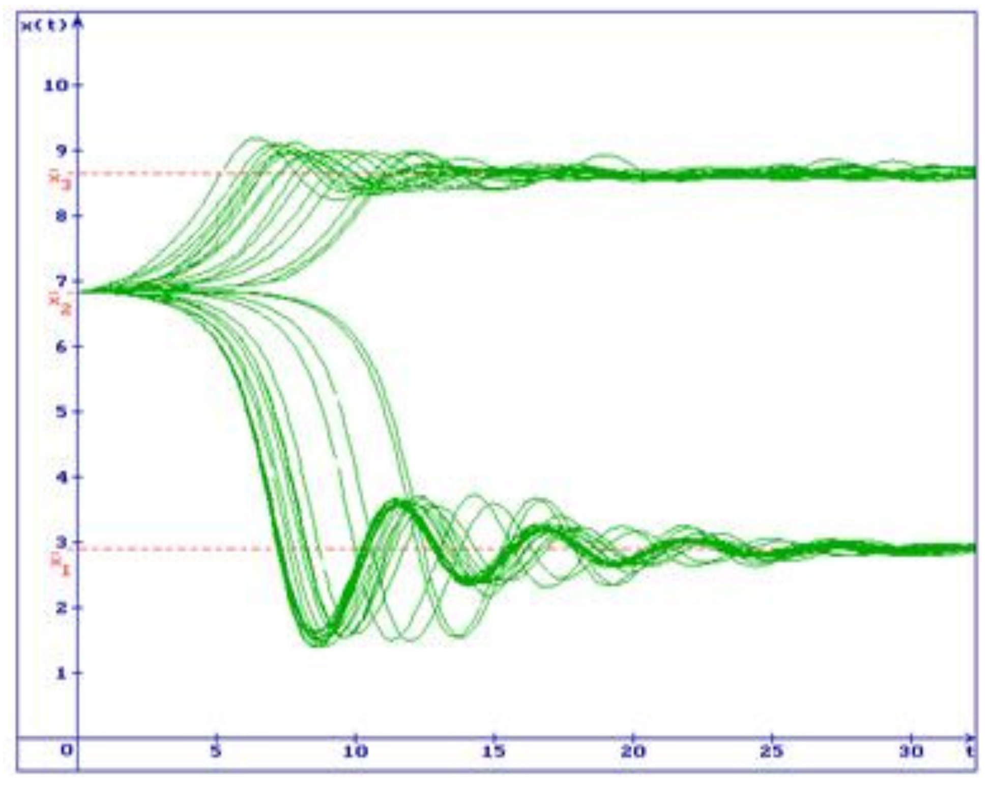
Consider the system (50) with , , , , , , , . In this case , , and . Thus, the first condition (7) does not hold and, consequently, the zero solution of the system (35) is unstable. By that, the equation (37) has three positive roots: , , , which are equilibria of the system (33) (Remark 5). For these equilibria we have respectively: , ; , ; , . Besides, , , . From Theorems 4 and 5 it follows that the equilibria and are stable in probability, the equilibrium is unstable. In Fig.3 50 trajectories of the system (50) solution are shown with the initial condition , , . One can see that all trajectories go out from the unstable equilibrium . By that, a part of the trajectories converges to the stable equilibrium , while another one converges to the stable equilibrium .
5. Conclusions
In this paper the classical problem of stabilization for the inverted pendulum is considered under stochastic perturbations of the type of Poisson’s jumps. The linear and nonlinear models are studied, stability conditions for the zero and nonzero equilibria are investigated. The obtained results are illustrated by numerical simulation of solutions of the equations under consideration. The proposed here research method can be used for detail investigation of many other nonlinear mathematical models in different applications.
Funding
This research received no external funding.
Conflicts of Interest
The author declares no conflict of interest.
References
- Acheson D.J. A pendulum theorem. Proceedings of the Royal Society of London, Seria A. Mathematical, Physical and Engineering Sciences, 1993, 443, 239-245. [CrossRef]
- Acheson D.J., Mullin T. Upside-down pendulums. Nature, 1993, 366(6452), 215-216. [CrossRef]
- Blackburn J.A., Smith H.J.T, Gronbech-Jensen N. Stability and Hopf bifurcations in an inverted pendulum. American Journal of Physics, 1992, 60(10), 903-908. [CrossRef]
- Borne P., Kolmanovskii V., Shaikhet L. Steady-state solutions of nonlinear model of inverted pendulum. Theory of Stochastic Processes, 1999, 5(21)(3-4), 203-209. Proceedings of the third Ukrainian-Scandinavian conference in probability theory and mathematical statistics, 8–12 June 1999, Kyiv, Ukraine.
- Borne P., Kolmanovskii V., Shaikhet L. Stabilization of inverted pendulum by control with delay. Dynamic Systems and Applications, 2000, 9(4), 501-514.
- Imkeller P, Lederer Ch. Some formulas for Lyapunov exponents and rotation numbers in two dimensions and the stability of the harmonic oscillator and the inverted pendulum. Dynamical Systems, 2001, 16(1), 29-61. [CrossRef]
- Kapitza P.L. Dynamical stability of a pendulum when its point of suspension vibrates, and pendulum with a vibrating suspension. In: ter Haar D (ed) Collected papers of P.L. Kapitza, vol 2. Pergamon Press, London, 714-737.
- Levi M. Stability of the inverted pendulum — a topological explanation. SIAM Review, 1988, 30(4), 639-644. [CrossRef]
- Levi M, Weckesser W. Stabilization of the inverted linearized pendulum by high frequency vibrations. SIAM Review, 1995, 37(2), 219-223. [CrossRef]
- Mata G.J., Pestana E. Effective Hamiltonian and dynamic stability of the inverted pendulum. European Journal of Physics, 2004, 25(6), 717-721.
- Mitchell R. Stability of the inverted pendulum subjected to almost periodic and stochastic base motion — an application of the method of averaging. International Journal of Nonlinear Mechanics, 1972, 7(1), 101-123. [CrossRef]
- Ovseyevich A.I. The stability of an inverted pendulum when there are rapid random oscillations of the suspension point. International Journal of Applied Mathematics and Mechanics, 2006, 70(5), 762-768. [CrossRef]
- Saleem O., Mahmood-ul-Hasan K. Robust stabilisation of rotary inverted pendulum using intelligently optimised nonlinear self-adaptive dual fractional-order PD controllers. International Journal of Systems Science, 2019, 50(7), 1399-1414. [CrossRef]
- Sanz-Serna J.M. Stabilizing with a hammer. Stochastics and Dynamics, 2008, 8(1), 47-57.
- Sharp R., Tsai Y-H., Engquist B. Multiple time scale numerical methods for the inverted pendulum problem. In: Multiscale methods in science and engineering. Lecture notes computing science and engineering, Springer, Berlin, 2005, 44, 241-261.
- Shaikhet L. Stability of difference analogue of linear mathematical inverted pendulum. Discrete Dynamics in Nature and Society, 2005, 2005(3), 215-226. Article ID 149487. [CrossRef]
- Shaikhet L. Improved condition for stabilization of controlled inverted pendulum under stochastic perturbations. Discrete and Continuous Dynamical Systems - A, 2009, 24(4), 1335-1343. [CrossRef]
- Shaikhet L. Lyapunov functionals and stability of stochastic difference equations. Springer Science & Business Media, 2011. https://link.springer.com/book/10.1007/978-0-85729-685-6.
- Shaikhet L. Lyapunov functionals and stability of stochastic functional differential equations, Springer Science & Business Media, 2013. https://link.springer.com/book/10.1007/978-3-319-00101-2.
- Gikhman I.I., Skorokhod A.V. Stochastic Differential Equations, Berlin: Springer-Verlag; 1972.
- Gikhman I.I., Skorokhod A.V. The theory of stochastic processes, v.III, Berlin: Springer-Verlag; 1979.
- Kolmanovskii V.B., Nosov V.R. Stability of Functional Differential Equations, Academic press, London, 1986.
- Kolmanovskii V.B., Myshkis A.D. Applied theory of functional differential equations, Kluwer Academic, Dordrecht, 1992.
- Kolmanovskii V.B., Myshkis A.D. Introduction to the theory and applications of functional differential equations. Kluwer Academic, Dordrecht, 1999.
- Mao X. Exponential stability of stochastic differential equations, Marcel Dekker, New York, 1994.
- Shaikhet L. Stability of the neoclassical growth model under perturbations of the type of Poisson’s jumps: analytical and numerical analysis. Communications in Nonlinear Science and Numerical Simulation, 2019, 72, 78-87. [CrossRef]
- Shaikhet L. About stabilization by Poisson’s jumps for stochastic differential equations. Applied Mathematics Letters, 2024, 153, 109068, 6 p. https://authors.elsevier.com/sd/article/S0893-9659(24)00088-0.
- Shaikhet L. Stability of difference analogues of nonlinear integro-differential equations: a survey of some known results. Research and Communications in Mathematics and Mathematical Sciences, Jyoti Academic Press, 2024, 16(1), 21-84.https://jyotiacademicpress.org/jyotic/journalview/16/article/66/112.
- Khasminskii R.Z. Stochastic stability of differential equations. Springer, 2012.
Figure 1.
Controlled inverted pendulum.
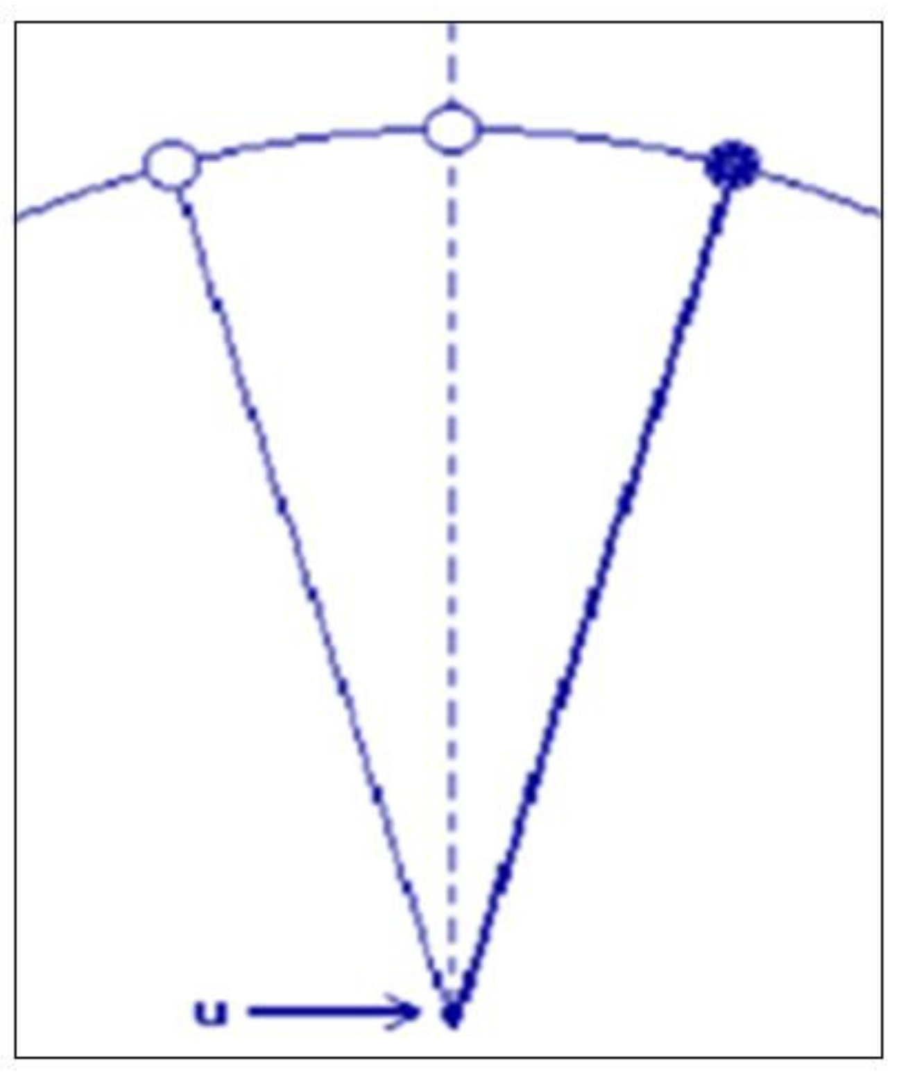
Figure 2.
50 trajectories of the solution of the system (46) , , , , , , , , , , , , .
Figure 2.
50 trajectories of the solution of the system (46) , , , , , , , , , , , , .
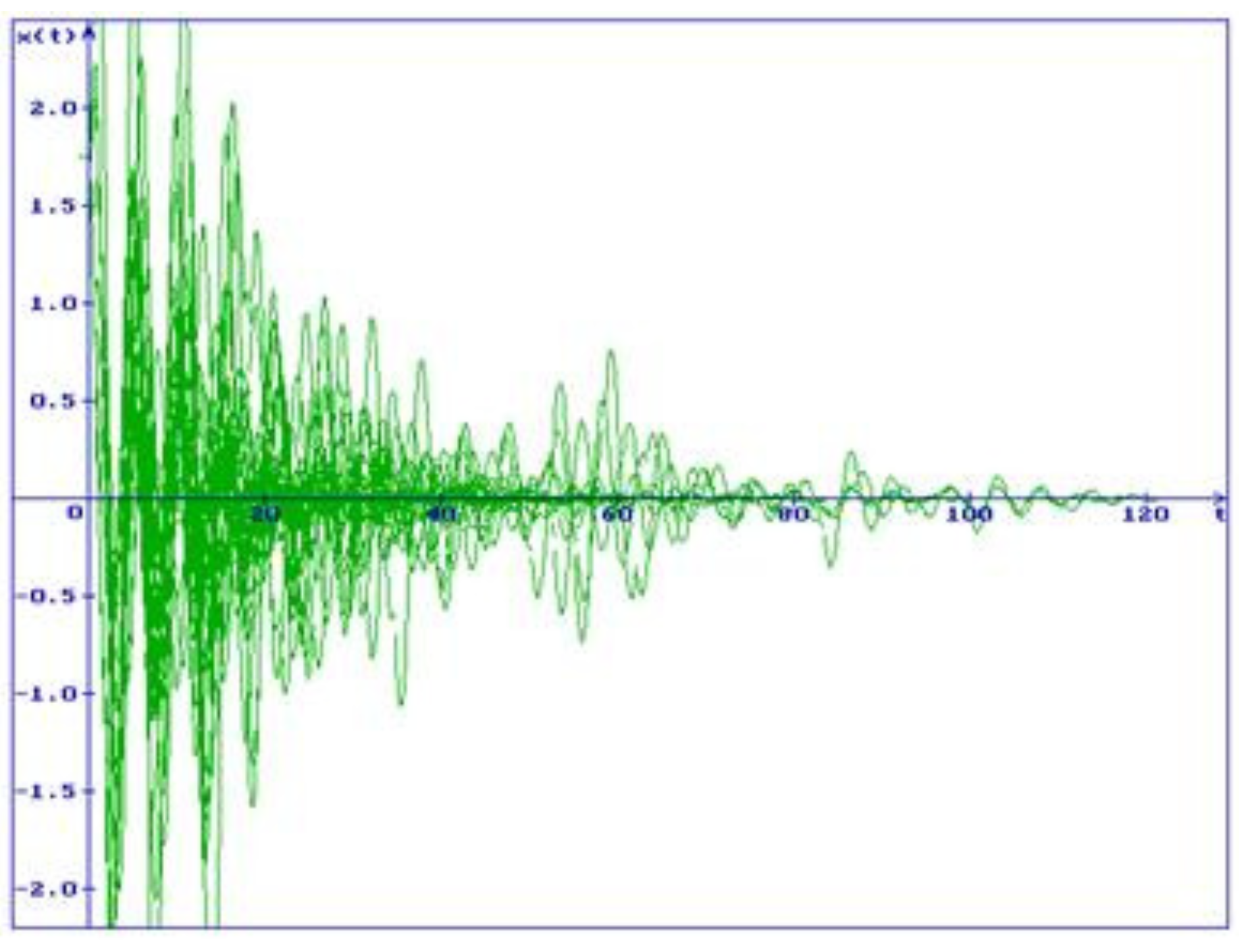
Figure 3.
50 trajectories of the solution of the system (50) , , , , , , , , , , , , .
Figure 3.
50 trajectories of the solution of the system (50) , , , , , , , , , , , , .
Disclaimer/Publisher’s Note: The statements, opinions and data contained in all publications are solely those of the individual author(s) and contributor(s) and not of MDPI and/or the editor(s). MDPI and/or the editor(s) disclaim responsibility for any injury to people or property resulting from any ideas, methods, instructions or products referred to in the content. |
© 2024 by the authors. Licensee MDPI, Basel, Switzerland. This article is an open access article distributed under the terms and conditions of the Creative Commons Attribution (CC BY) license (http://creativecommons.org/licenses/by/4.0/).
Copyright: This open access article is published under a Creative Commons CC BY 4.0 license, which permit the free download, distribution, and reuse, provided that the author and preprint are cited in any reuse.


