
Submitted:
26 November 2024
Posted:
27 November 2024
You are already at the latest version
Abstract
The management and classification of solid waste is one of the most important challenges worldwide. The objective is to design a basic waste classification system at the source using a low-cost experimental capacitive sensor and Machine Learning algorithms. For this, two types of sensor models were established (Traditional Model (MT) and Non-Traditional Model (MNT)), which were built with recyclable material and tested with different types of materials, in order to evaluate their behavior and sensitivity level. According to the results obtained, it was possible to show that the two sensors responded with adequate levels of sensitivity for each of the materials used as a test, however, the MNT model was the one that generated the values with the greatest variability, an aspect that is considered of great relevance, because, thanks to this type of response to various types of materials, it facilitates the classification processes through the use of Machine Learning algorithms. Finally, the two prototypes of sensors manufactured can be considered of great importance for the development of more complex solutions, related to the classification and possible characterization of materials, in comparison with the capacitive sensors found on the market, which only they allow to identify if there is presence or not of some object through adjustment by potentiometer, generating as a result a digital output. This aspect largely limits the use of commercial capacitive sensors to applications exclusively related to presence or level detection.
Keywords:
sensor
; capacitive
; solid waste
; machine learning
; artificial intelligence
1. Introduction
Solid waste management stands among the most pressing global challenges today. The generation of waste has steadily increased, driven by factors such as rapid population growth, accelerated industrialization, and economic development [1]. This trend has given rise to a series of environmental and social problems, particularly regarding public health and the conservation of the natural environment [2]. Proper waste management is essential to mitigate these negative effects, requiring the implementation of efficient processes that encompass waste collection at the source, transportation, treatment, segregation, and final disposal [3]. Developing countries, in particular, face the challenge of optimizing these processes, whose effectiveness largely depends on the knowledge and resources available to the institutions responsible for their implementation [4].
Within the framework of environmental policies, solid waste management holds a fundamental position. Its proper implementation aims not only to reduce environmental impact but also to improve living conditions, prevent public health issues, and promote sustainability [5]. Solid waste classification has gained prominence as a key measure to achieve sustainable economic development goals, reduce poverty, and preserve ecosystems. The adoption of efficient solid waste classification systems is crucial to creating jobs, stimulating the recycling sector, and fostering social well-being [6]. Therefore, efforts must focus on improving waste separation practices at the source, benefiting both the environment and the communities that rely on these economic activities.
Given this scenario, there is a need to develop innovative technologies that optimize waste classification at its origin, enabling a more effective resolution of this issue. With the advancement of emerging technologies such as the Internet of Things (IoT) and Artificial Intelligence, governments worldwide are working toward the creation of "smart cities," where efficient waste management plays a fundamental role [7]. These technologies have great potential to automate and optimize waste classification processes. However, most solutions developed for waste classification focus on image recognition using techniques such as Convolutional Neural Networks, optical methods, and spectrophotometry, among others [8,9,10,11,12,13]. While these methods offer high levels of effectiveness, they often require expensive equipment and are, in many cases, sensitive to the presence of impurities. This makes them unsuitable for environments with high levels of contamination, such as waste collection points, significantly increasing implementation costs and limiting their large-scale adoption.
In this context, the present article proposes an innovative solution through the development of a low-cost capacitive sensor with the capability and sensitivity to facilitate the classification of various types of solid waste at the source, including glass, plastic, metal, and organic waste. This solution utilizes machine learning algorithms, offering an efficient and sustainable alternative to this pressing issue.
2. Materials and Methods
2.1. Solid Waste Classification
The classification or segregation of solid waste is considered by numerous studies as one of the fundamental pillars of the Solid Waste Management System [14]. These wastes are composed of materials, many of which are recyclable, such as paper, cardboard, glass, plastic, rubber, and ferrous and non-ferrous metals, which can be reused in various industrial processes. On the other hand, organic waste has the potential to be transformed for the production of biogas and biofertilizers. However, due to inadequate waste management and incorrect collection practices, common in many cities, serious social, health and environmental problems have been generated, in addition to economic, resource and energy losses [15]. As a consequence of this poor management, recycling rates are extremely low and the amount of waste deposited in landfills exceeds their capacity, which negatively impacts society and the natural environment.
When talking about the correct way to separate waste, the method best known and implemented by institutions and at the domestic level is the manual classification method, which consists of depositing waste in different containers taking into account their material, this method is supported by pedagogy programs that instruct people on the subject [16]. However, the technology of garbage sorting and environmental monitoring has developed rapidly in recent years, where the combination of the Internet of things, artificial intelligence and environmental technology has become a trend for solving environmental problems. and social [17].
2.2. Sensors
A sensor is a device that is used to measure or detect a change in the environment or in a physical variable under study, which will deliver an output value under a specific format [18]. An analog sensor produces a voltage or continuous output signal, which is generally proportional to the quantity being measured. Digital sensors, on the other hand, produce discrete digital output signals or voltages that are a digital representation of the quantity being measured. Digital sensors produce a binary output signal in the form of a logic "1" or a logic "0", ("ON" or "OFF") or can be represented as a "byte" (8 bits).
2.3. Capacitive Sensor
Capacitive proximity sensors are devices that, without the need for contact, allow detecting the presence or absence of practically any object regardless of the material (glass, paper, metal, plastic, biological, etc.). They use the electrical property called "capacitance", where by means of a change in the electric field produced by the object under observation ("dielectric"), it generates a change in the value of the resulting capacitance, thereby facilitating the detection of an object and the possibility of identifying the type of material that composes it [8]. Figure 1 shows the appearance of the Capacitive Sensor.
When an object is located within the sensitive zone, an alteration of the electric field is produced, varying the resulting capacitance and therefore the frequency of the oscillator. There are two categories of targets that capacitive sensors can detect: the first is conductive and the second is non-conductive. Conductive targets include metal, water, blood, acids, bases, and salt water, among other similar materials. These targets have a higher capacitance and the dielectric strength of the targets is irrelevant [19]. When it comes to metallic elements, the electric field decreases since a phenomenon equivalent to series capacitances occurs.
On the other hand, when dealing with a non-conductive target, it acts as an insulator for the electrode of the sensors. A target dielectric constant, also sometimes called a dielectric constant, is the measure of insulation properties used to determine the sensing distance reduction factor. For non-metallic objects, there is an increase in the electric field due to the increase in the dielectric constant. Capacitive sensors are normally used for the detection of non-metallic materials such as: Glass, oil, water, cardboard, ceramics, plastic, wood, paper, among others [20].
Although there are several very high-precision methods for measuring parameters related to magnetic permeability, electrical permittivity, and conductivity of a material, among which microwave measurement methods stand out, these are usually very expensive to implement in materials and equipment, which is why they are not considered suitable for the solution required for the problems associated with the identification of materials for the classification of waste at the source. Given this situation, it is considered feasible to carry out the classification process alternately, using a low-cost sensor, articulated with classification techniques based Machine learning algorithms.
2.4. Design of the Proposed Capacitive Sensors
For the fabrication of the two proposed sensors, recycled aluminum sheets from beer cans were utilized. This material was selected due to its accessibility, reusability, and alignment with the overarching objectives of the project. It is important to note that beer or soft drink cans can be made of either steel or aluminum, depending on the application and the production region, where the availability of these materials may vary. However, in most cases, cans are made of aluminum, as in this study, due to its effectiveness in preserving beverages by protecting them from air, light, and potential contamination risks, including bacteria, viruses, hazardous chemicals, and physical agents.
Moreover, aluminum is an economical and sustainable material, thanks to its high recyclability [21]. Cans are typically coated with a thin layer of paint and plastic. The plastic serves to separate the beverage from the aluminum, preventing chemical reactions between the liquid and the metal or contamination from direct contact. The most common plastics used for this type of coating include polyethylene (PE), polypropylene (PP), polystyrene (PS), polyethylene terephthalate (PET), and polyvinyl chloride (PVC). As an insulating material, plastic possesses a relative electrical permittivity, which directly influences the capacitance value of each sensor. Table 1 provides the relative electrical permittivity values for the aforementioned types of plastic [22].
During the construction process of the MT and MNT sensors, a plastic layer (polypropylene) was used as protection against the environment in which they will be used, establishing a value of . In addition, this layer allowed maintaining a constant distance between the plates, avoiding direct contact between them.
2.4.1. Sensor Design MT
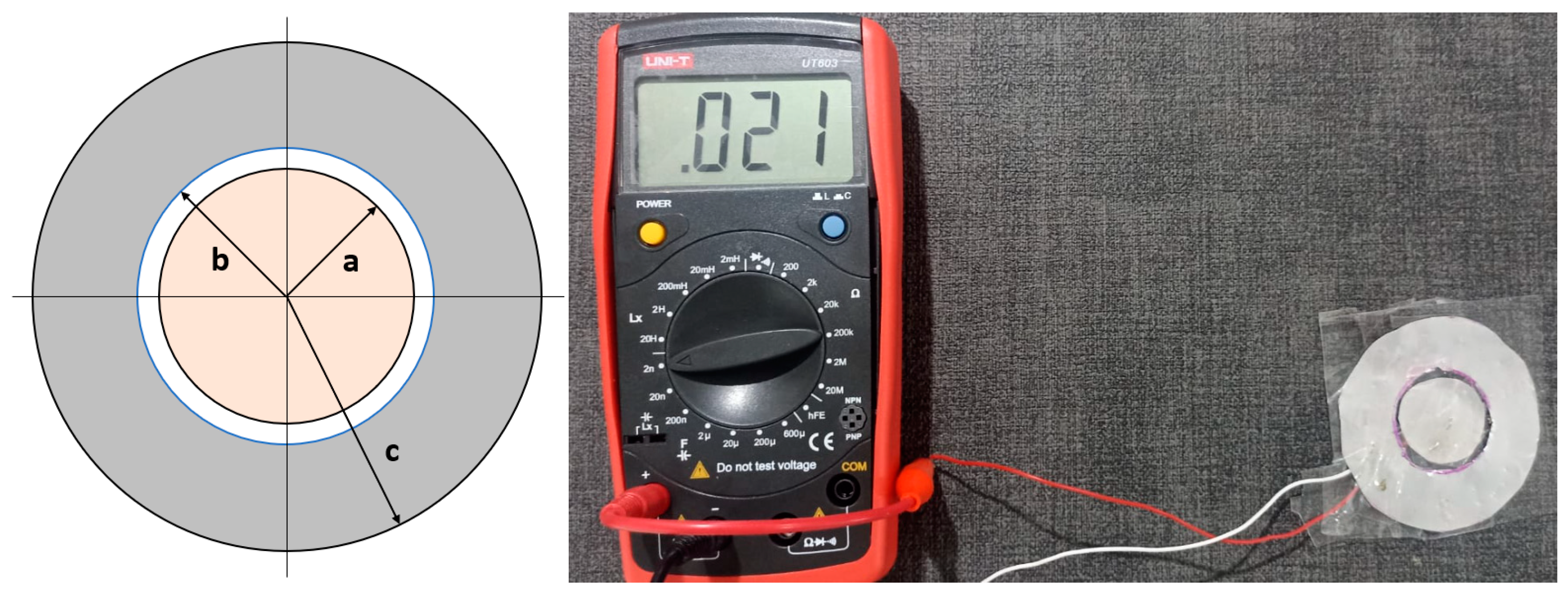
This sensor is made up of two concentric plates, where one of the plates is circular with radius a and the other plate has the shape of a circular crown with inner and outer radii b and c respectively. Figure 2 shows the proposed diagram for the MT sensor, accompanied by the distribution of electrical charges on each of the plates and electric field lines, in order to establish the conditions and key elements for estimating the capacitance value.
For the process to estimate the Capacitance value for the MT sensor model, it begins with equation (1), which corresponds to Gauss' Law [23], which defines the mathematical expression that allows calculating the electric field (E), by defining a Gaussian surface radius (r) containing the total charge of the capacitor (q) uniformly distributed over the surface area (A) and electrical permittivity .
Where,
Electrical permittivity in a vacuum ()
Relative permittivity of the dielectric between the plates of the capacitor.
Solving for the electric field and replacing the area of the circumference
( in expression (1) results in equation (2):
Subsequently, we proceed to define the mathematical expression that allows us to calculate the value of the voltage (V) existing between points a and b. The result of this process is described in equation (3):
Finally, the value of the capacitance for the MT sensor () is given by the relationship between the total charge () and the voltage (V), as presented in equation (4):
2.4.2. MNT Sensor Design
This sensor consists of two "E" shaped plates, a design inspired by that of a resistive humidity sensor. In this case, both the area of the plates () and the number of slots interspersed between them are equal, and are separated by a distance (d). Figure 4 presents the proposed diagram for the MNT sensor, whose parameters are defined by the dimensions a, b, c and d. Furthermore, Figure 3 illustrates how the positive and negative electric charges are distributed on the plates of the capacitive sensor, showing the electric field lines and their similarity to the model of a parallel plate capacitor, characterized by an area (A) and separation (d).
Therefore, the capacitance value for the MNT capacitive sensor can be calculated from equation (5):
3. Results
3.1. Comparative Analysis of Theoretical and Experimental Capacitance for MT and MNT Sensors
In the experiment, a UNI-T UT603 digital capacitance and inductance meter (LCR) with a tolerance of 1% was used to determine the capacitance in pF of each of the proposed sensors, considering the conditions and type of waste material.
Figure 4 shows a capacitance value delivered by the LCR for the implemented prototype of the MT Sensor, when it is free of residues, accompanied by the proposed diagram. From equation (4), we proceed to calculate the capacitance value according to the sensor dimensions that were considered at the discretion of the researchers for its construction (a=2.1 cm, b=2.3 cm, c=3 cm and d=0.2 cm).
Equations (6 - 8) present the result of this process accompanied by the absolute error ( and the relative error () [24] in contrast to the result obtained experimentally, where it can be seen that the theoretical value and the one obtained experimentally are very similar to each other, with reduced error levels taking into account that the capacitance values are of the order of , an aspect that is very common in commercial capacitors, which establish a tolerance value given by the manufacturer and considering that the relative permittivity values of the materials used for the construction of the sensors may vary a little compared to those that were theoretically adopted.
Figure 4.
Capacitance value with Prototype Sensor Traditional Model (MT) without residuals for reading.
Figure 4.
Capacitance value with Prototype Sensor Traditional Model (MT) without residuals for reading.
The proposed diagram and the capacitance value of for the implemented MNT sensor prototype, when free of residues, are presented in Figure 5. Using Equation (5), the capacitance value is determined based on the sensor's dimensions, which were selected by the researchers during its construction (a=5 cm, b=0.9 cm, c=1.5 cm and d=0.1 cm).
The results of this process are presented in equations (9 - 11), together with the absolute error ( and the relative error () in comparison with the results obtained experimentally. It can be observed that the theoretical and experimental values are very similar, as in the previous case, showing low levels of absolute and relative error. From this, it can be concluded that the mathematical expressions proposed for each type of sensor are consistent with the experimental results, which allows establishing a valuable reference point for future research in which it is planned to use any of the proposed models or make modifications regarding their design or dimensions.
3.2. Estimation of the Number of Samples and Analysis of the Information
To carry out the sampling campaigns, the estimation of the sample size required for two independent samples was made, since they are two different sensors (MT and MNT), establishing a power of the test (, a confidence level of the 95% ( and an effect size of 0.5 [25]. By using the XLSTAT tool, a minimum size of 85 was obtained as a result for each sample. In view of the above and in order to establish a more significant number of samples for each of the four different types of waste to be classified, accompanied by For a better result in terms of statistical indicators, related to the power of the test and the confidence level, an amount of 100 samples was established for each type of sensor (200 samples in total), where each cluster of 100 samples contains 25 records for each of the four types of waste or materials (plastic, glass, metal and organic). Table 2 and Table 3 show the mean, standard deviation and confidence intervals for each characteristic, according to the type of material or waste used during the sampling campaign depending on the type of sensor.
Figure 4, Figure 5, Figure 6 and Figure 7 present some of the results obtained during the measurement campaigns, both in the absence of material or waste (figures 4 and 5), and in the presence of reusable waste such as: plastic, glass and metal, as well as in various types of organic waste. Figure 4 and Figure 6 show some of the results recorded in terms of Capacitance using the MT capacitive sensor, registering a value of 21pF in the absence of material or residue. In turn, values between 22 and 27 pF for reusable materials and values between 80 and 450pF when dealing with organic waste. On the other hand, figures 5 and 7 present some of the results in terms of Capacitance for the MNT capacitive sensor, registering a value of 28pF in the absence of material or residue. In turn, values between 31 and 37 pF for reusable materials and values between 150 and 1200pF when dealing with organic waste.
Figure 6.
Records with Sensor - Traditional Model (MT) for various types of waste.
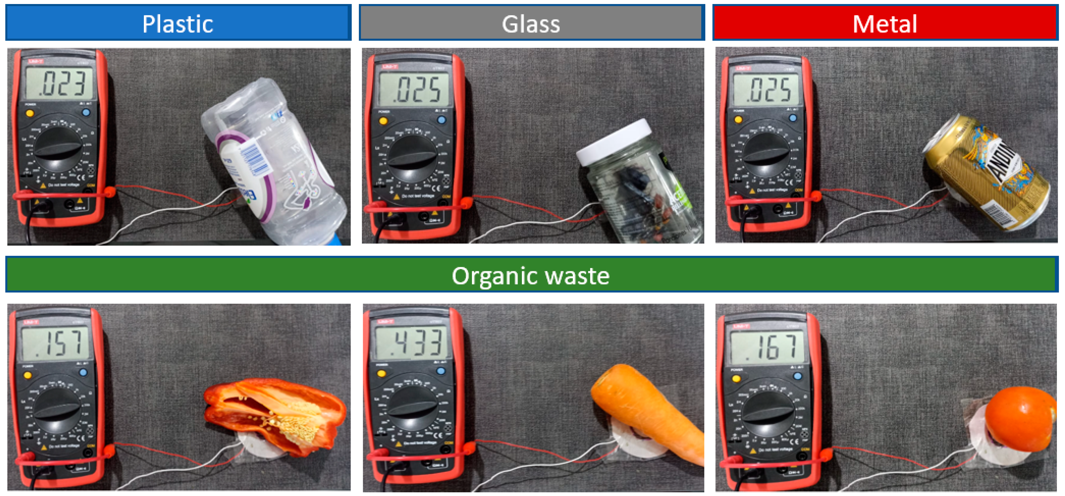
Figure 7.
Records with Sensor - Non-Traditional Model (MNT) for various types of waste.
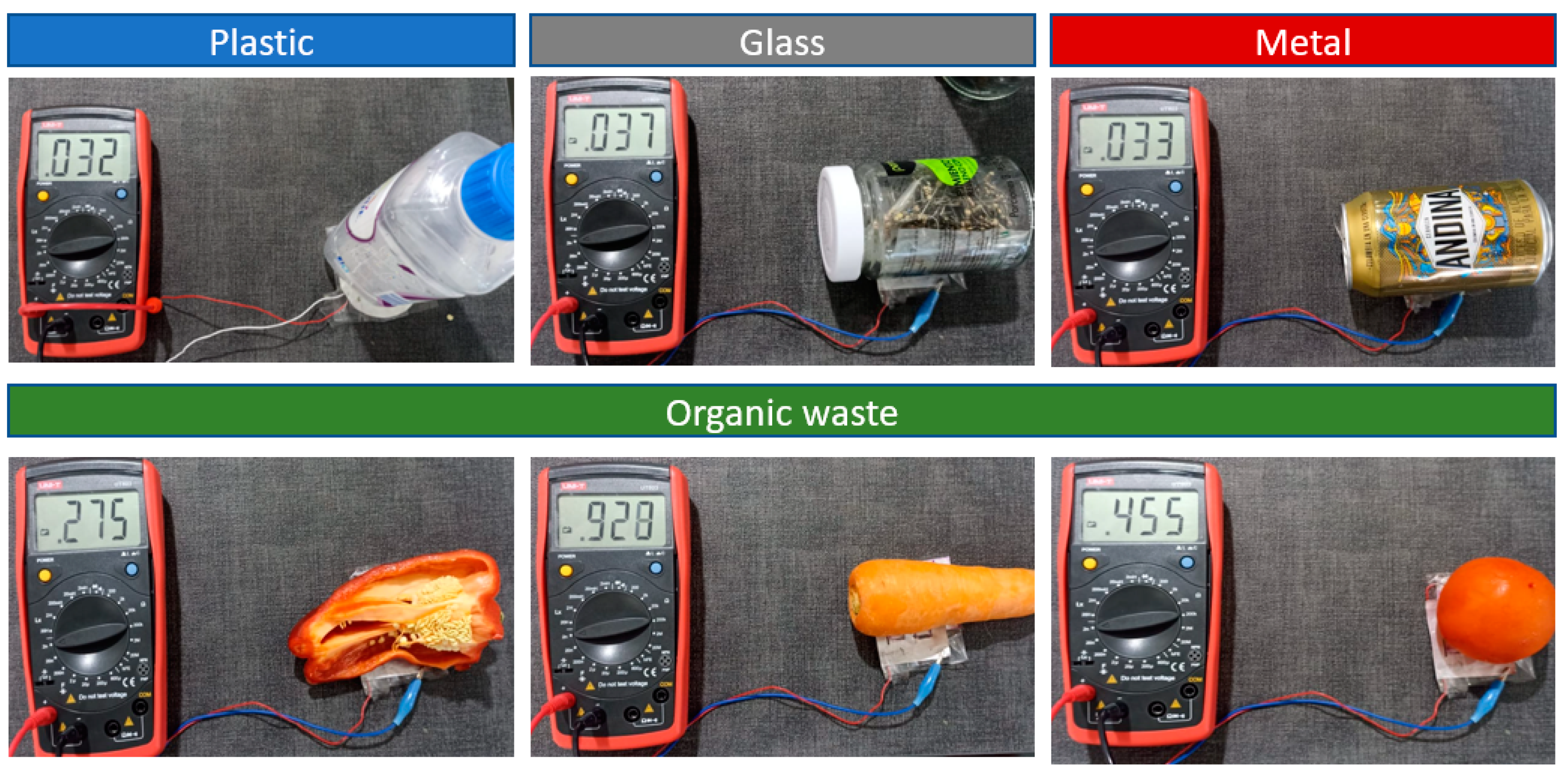

Table 2.
Statistical results of capacitance measurements with Sensor MT.
| Material | Capacitance [pF] | ||
|---|---|---|---|
| Mean | Standard deviation | Confidence interval (95%) | |
| Plastic | 24.680 | 1.519 | (24.084, 25.275) |
| Glass | 25.080 | 1.394 | (24.538, 25.622) |
| Metal | 25.120 | 1.394 | (24.573, 25.666) |
| Organic | 251.120 | 120.823 | (203.757, 298.482) |
Table 3.
Statistical results of capacitance measurements with Sensor MNT
| Material | Capacitance [pF] | ||
|---|---|---|---|
| Mean | Standard deviation | Confidence interval (95%) | |
| Plastic | 34.680 | 1.574 | (34.063, 35.297) |
| Glass | 34.880 | 1.666 | (34.227, 35.533) |
| Metal | 31.960 | 0.934 | (31.593, 32.326) |
| Organic | 680.960 | 324.396 | (553.799, 808.120) |
In order to visually describe the way in which the data that are part of the data recorded during the sampling campaigns are distributed, as well as to estimate the levels of variability for each of the different types of residues that were considered as reference In order to evaluate the behavior of each one of the proposed sensors, as well as the purification of the information in terms of identification of atypical data, box diagrams were carried out for each particular case, and the results of which are available in Figure 8 and Figure 9.
Additionally, the possibility was considered that the size of the sample that was established for the development of the project could have affected in some way the appearance of each of the resulting figures. However, from a practical point of view, according to [26], it is possible to consider that a box plot can be reliable as long as the sample size established for each item is equal to or greater than 20. Taking into account that 25 samples were established for each type of residue, it can be considered that this recommendation is fulfilled and with this the result of each figure can be considered reliable.
Figure 8.
Plot of boxes related to Capacitance [pF] for the MT sensor
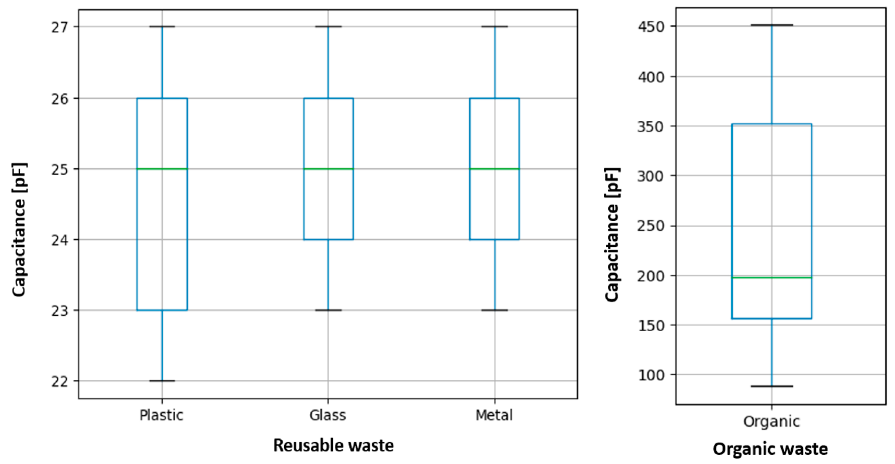
Figure 9 and Figure 10 show the box diagrams related to the Capacitance [pF] recorded by the MT and MNT sensors. In them it can be seen that the behavior of the capacitance for the readings recorded by the MNT sensor describe a normal distribution for the case of the three types of reusable waste (plastic, glass and metal), a situation that occurs in a similar way with waste. corresponding to glass and metal in the case of the MT sensor. However, for the particular case of plastic in the MT sensor, it describes a positive asymmetry, describing a higher concentration of the values recorded between 50 and 75%.
Figure 9.
Plot of boxes related to Capacitance [pF] for the MNT sensor
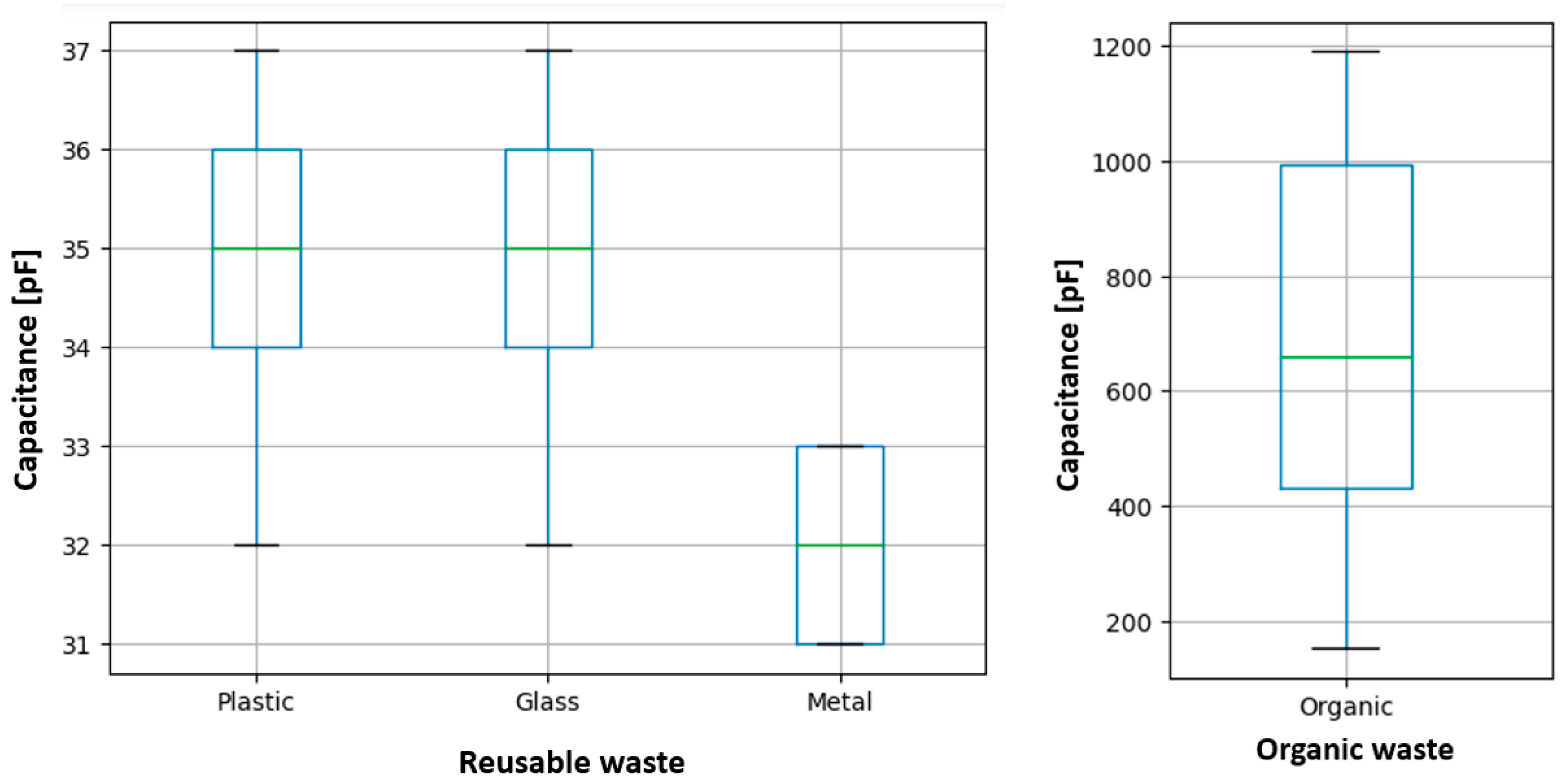
This is not the case for the organic residues for the two sensors, where a negative asymmetry is observed, thus establishing an indication of a higher concentration of readings for this type of residues between the Q1 and Q2 quartiles, a phenomenon that describes a higher incidence in the MT sensor. In turn, the readings related to Plastic for the MT sensor slightly show a higher level of dispersion compared to the readings of the other reusable waste for both types of sensors. Additionally, it can be seen that the values corresponding to the median for the readings recorded by the MT sensor for reusable waste present a common value of approximately 25 [pF] in the three cases, an aspect that occurs similarly for the MNT sensor, where the Waste related to Plastic and Glass describe a median value or Q2 of 35 and for metal a value of approximately 32. For the particular case of organic waste, approximate values are obtained for the MT and MNT sensors of 200 and 660 respectively, with a higher level of dispersion for the case of the MNT sensor.
The comparative statistical analysis of the MT and MNT sensors reveals significant differences in capacitance measurement for different materials, with the MNT sensor's performance standing out due to its greater dynamic range. For reusable materials (plastic, glass and metal), both sensors show relatively homogeneous capacitance values, with similar means and low standard deviations. However, the 95% confidence intervals (CI) of the MNT sensor are slightly wider, which could be attributed to greater sensitivity in the measurement. For example, for glass, the MT sensor presents a CI of (24.538, 25.622), while the MNT sensor widens it to (34.227, 35.533), indicating a shift towards higher capacitance values and a more differentiated measurement between materials.
For organic waste, the superiority of the MNT sensor is evident due to its ability to capture higher capacitance values and greater relative variability, thereby reducing the overlap with reusable materials. The MT sensor records a mean of 251.120 pF with a standard deviation of 120.823 and a wide CI of (203.757, 298.482), while the MNT sensor reaches a mean of 680,960 pF with a standard deviation of 324.396 and a CI of (553.799, 808.120). Not only does this demonstrate that the MNT sensor can more effectively differentiate organic waste from the rest, but its greater dynamic range, as quantified by the ratio of means to standard deviations (coefficient of variation), strengthens its classification capability. In organic waste, the coefficient of variation for the MT sensor is 48.1%, while for the MNT sensor it rises to 47.6%, indicating that, although both present high dispersion, the MNT sensor is more effective in separation thanks to its greater width in the distribution of values.
3.3. Comparison of MT vs. MNT Treatments
Let and be the recorded capacitance values (most relevant characteristic) for each MT and MNT sensor respectively and , is the difference between samples. In order to evaluate whether the MNT sensor describes a better behavior compared to the MT sensor, the following hypotheses are posed:
Where and are the means corresponding to the capacitance values obtained during the sampling campaigns for the two types of MT and MNT sensors respectively. The hypothesis, states that MNT is better than the MT model and the establishes the opposite condition. To accept or reject the proposed hypotheses, it is necessary to perform a hypothesis contrast on the difference in means with paired sampling, using the so-called paired t-test. For this, the following steps are established[27]:
- Step 1: A new random variable is defined and the mean value and standard deviation for the variable are calculated. The result of this process yielded the values of and for and respectively. On the other hand, when defining a new variable Z, it is necessary to make an adjustment in the hypotheses as follows:
- Step 2: We proceed to calculate the value of the statistic established for the test by using the following expression:
Where d is the value of the statistic and n obeys the number of samples for the two proposed scenarios.
- Step 3: Establish the acceptance range of the for at 5% significance (and degrees of freedom. For the particular case, the value of , defining the range of acceptance of the between . When evaluating the value of the d statistic, it is observed that it is within the acceptance interval, which is why is not rejected. In view of the above, it is concluded that the sensor supported in the MNT model is better than the MT sensor for the proposed scenario, with 95% confidence. Additionally, the MNT sensor describes a higher variance (greater response sensitivity, in the presence of different types of materials and even of the same type) compared to the MT sensor, which is very favorable for the identification and classification of waste or materials.
3.4. Classification of Solid Waste with MNT Sensor Using Machine Learning Algorithms
Among the various classification algorithms available in Machine Learning, the Random Forests model was selected to carry out the classification process using the MNT sensor. The training, testing and validation phases were carried out using the data set collected during sampling campaigns with the MNT sensor, consisting of 100 records with capacitance (pF) as a feature distributed into two classes: reusable waste (Class 0) and organic waste (Class 1). The data analysis processes were implemented using Python libraries such as sklearn, matplotlib, pandas, numpy and scipy, through the Google Colab platform. Additionally, to ensure bias-free model training, the RobustScaler normalization technique of the sklearn library was applied and the train_test_split function was used to split the dataset into training and test subsets.
Figure 10 presents the confusion matrix obtained for the Random Forests model, in which there were no false positive or false negative records, correctly classifying the 75 records belonging to Class 0 (reusable waste) and the 25 records of Class 1 (organic waste), demonstrating adequate levels of precision and reliability during the classification process according to the reading made by the sensor. In turn, performance metrics such as accuracy, precision, recall and F1-score were calculated for the Random Forests model, obtaining a perfect value of 1.0 in all cases. This result reflects optimal performance. Additionally, the absence of overfitting was validated by the consistency of all metrics, thus avoiding relying solely on the accuracy metric, which can be misleading under bias conditions.
Figure 10.
Confusion matrix obtained for the Random Forests model
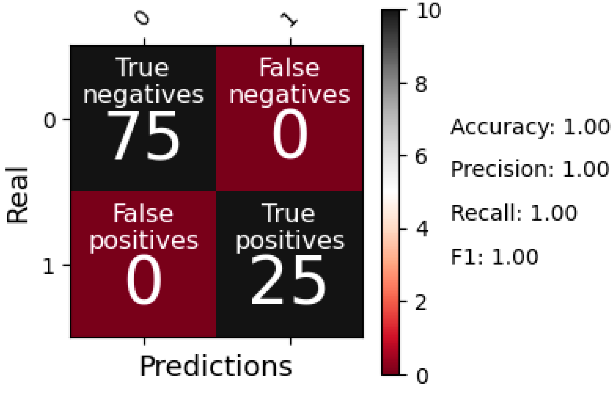
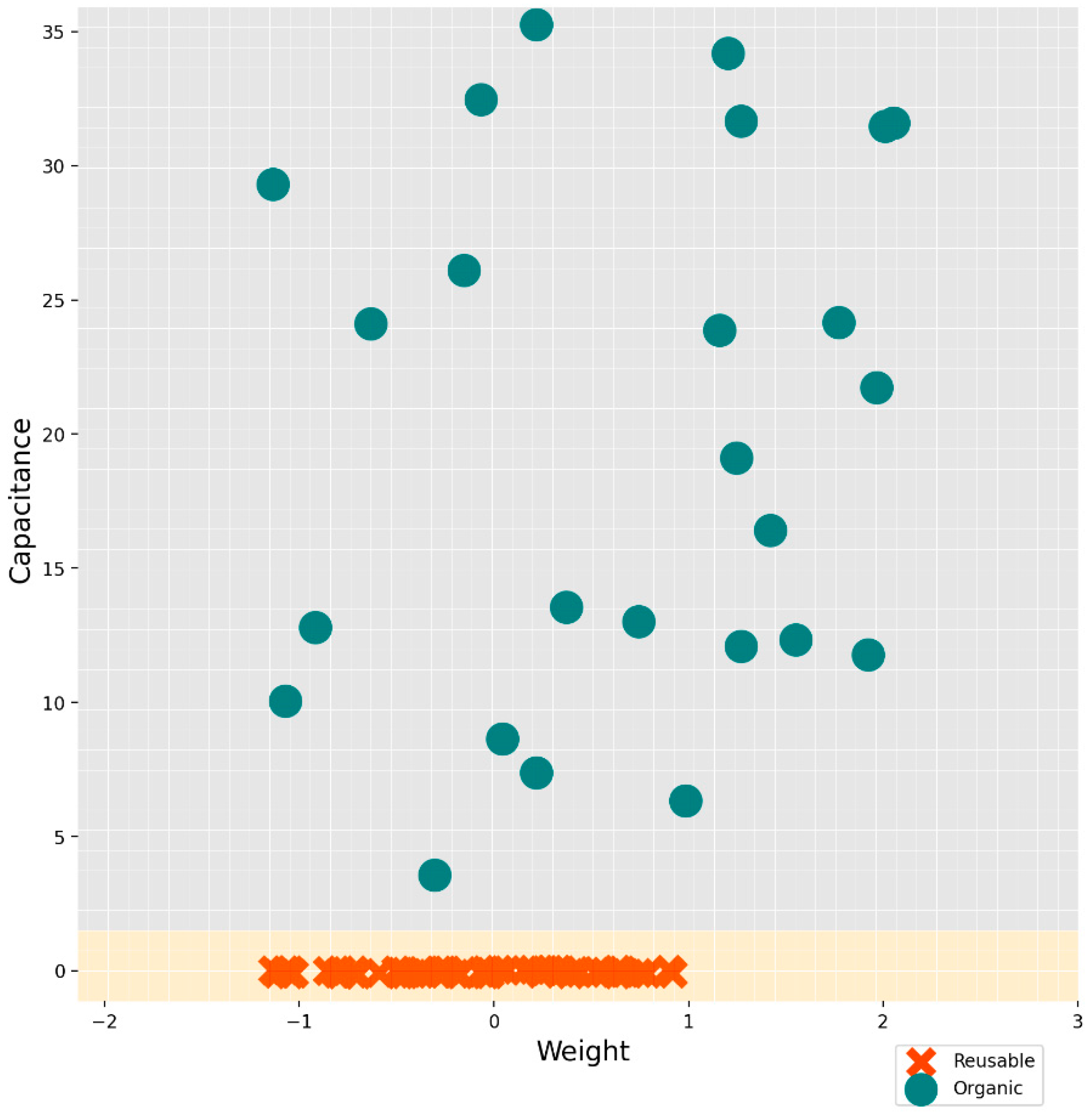
Figure 11 presents the graphic validation of the proposed classification model, in which the decision limits used to separate the waste classes can be clearly seen. In turn, the reference line observed horizontally reflects consistent thresholds for the capacitance values corresponding to each type of waste. Finally, for both reusable and organic waste, the capacitance thresholds are in an intermediate tolerance zone, which significantly reduces the risk of incorrect classification when the new data deviate slightly from the values established during the training process.
Figure 11.
Validation of the Random Forest
4. Conclusions
Within the broad spectrum of problems related to environmental protection, solid waste management occupies one of the most important places within environmental management policies, where the main objective is to establish mechanisms that allow this process to be carried out efficiently and compatible with the environment and public health. For this reason, the use of technologies such as capacitive sensors and Artificial Intelligence could help to implement economic and efficient solutions that allow the classification of solid waste at the source, minimizing the time necessary for its classification compared to separation processes manuals, reduce the health risks that may arise when working with contaminated waste and increase the percentage of waste that can be reused and reprocessed later thanks to the proper separation process. According to the results obtained, it was possible to show that the two models of capacitive sensors proposed describe an adequate behavior in terms of sensitivity and coherence with the readings registered for each type of material or test residue that was used for its evaluation. However, the MNT sensor model was the one that described the best behavior in relation to sensitivity and variability for each type of waste, with 95% confidence, allowing waste classification processes through the use of Machine algorithms. Learning, establishing an economic and reliable alternative for the implementation of this type of solutions at the source and in turn promoting the development of future projects related to the classification of materials in a more selective way, which could be oriented to the separation of reusable waste such as glass, paper, plastic, metal, among others independently or for the specific characterization of materials, with possible industrial applications.
Author Contributions
J.C.V.F.: Conceptualization, methodology, software, validation, formal analysis, investigation, data curation, supervision, project administration and funding acquisition; H.E.P.: validation, investigation, data curation, and supervision; J.A.V.: resources, visualization, supervision, project administration, and funding acquisition. All authors have read and agreed to the published version of the manuscript.
Funding
The authors appreciate the financial support provided by UNAD (PG0501ECBTI2022) and the company Smarttic during the development of this study.
Institutional Review Board Statement
Not applicable
Informed Consent Statement
Not applicable
Data Availability Statement
The raw data supporting the conclusions of this article will be made available by the authors on request.
Conflicts of Interest
The authors declare no conflicts of interest.
References
- Pan, Z.; Sun, X.; Huang, Y.; et al. Anaerobic Co-Digestion of Food Waste and Microalgae at Variable Mixing Ratios: Enhanced Performance, Kinetic Analysis, and Microbial Community Dynamics Investigation. Appl Sci 2024, Vol 14, Page 4387. 2024;14(11):4387. [CrossRef]
- Gan, B.; Zhang, C. Research on the algorithm of urban waste classification and recycling based on deep learning technology. In: Proceedings - 2020 International Conference on Computer Vision, Image and Deep Learning, CVIDL 2020. Institute of Electrical and Electronics Engineers Inc.; 2020:232-236. [CrossRef]
- Kokoulin, A.N.; Uzhakov, A.A.; Tur, A.I. The Automated Sorting Methods Modernization of Municipal Solid Waste Processing System. In: Proceedings - 2020 International Russian Automation Conference, RusAutoCon 2020. Institute of Electrical and Electronics Engineers Inc.; 2020:1074-1078. [CrossRef]
- Dadic, B.; Ivankovic, T.; Spelic, K.; Hrenovic, J.; Jurisic, V. Natural Materials as Carriers of Microbial Consortium for Bioaugmentation of Anaerobic Digesters. Appl Sci 2024, Vol 14, Page 6883. 2024;14(16):6883. [CrossRef]
- Colasante, A.; D’Adamo, I. The circular economy and bioeconomy in the fashion sector: Emergence of a “sustainability bias.” J Clean Prod. 2021;329. [CrossRef]
- Blumberga, D.; Ozarska, A.; Indzere, Z.; Chen, B.; Lauka, D. Energy, Bioeconomy, Climate Changes and Environment Nexus. 2019;23(3):370-392. [CrossRef]
- Saranya, M. A Survey on Health Monitoring System by using IOT. Int J Res Appl Sci Eng Technol. 2018;6(3):778-782. [CrossRef]
- Dhulekar, P.; Gandhe, S.T.; Mahajan, U.P. Development of Bottle Recycling Machine Using Machine Learning Algorithm. In: 2018 International Conference On Advances in Communication and Computing Technology, ICACCT 2018. Institute of Electrical and Electronics Engineers Inc.; 2018:515-519. [CrossRef]
- Lin, W. YOLO-Green: A Real-Time Classification and Object Detection Model Optimized for Waste Management. Proc - 2021 IEEE Int Conf Big Data, Big Data 2021. Published online 2021:51-57. [CrossRef]
- Saranya, A.; Bhambri, M.; Ganesan, V. A Cost-Effective Smart E-Bin System for Garbage Management Using Convolutional Neural Network. 2021 Int Conf Syst Comput Autom Networking, ICSCAN 2021. Published online July 30, 2021. [CrossRef]
- Liu, K.; Liu, X. Recycling Material Classification using Convolutional Neural Networks. Proc - 21st IEEE Int Conf Mach Learn Appl ICMLA 2022. Published online 2022:83-88. [CrossRef]
- Faria, R.; Ahmed, F.; Das, A.; Dey, A. Classification of Organic and Solid Waste Using Deep Convolutional Neural Networks. IEEE Reg 10 Humanit Technol Conf R10-HTC. 2021;2021-September. [CrossRef]
- Nagajyothi, D.; Ali, S.A.; Jyothi, V.; Chinthapalli, P. Intelligent Waste Segregation Technique Using CNN. 2023 2nd Int Conf Innov Technol INOCON 2023. Published online 2023. [CrossRef]
- Wang, B.; Zhou, W.; Shen, S. Garbage classification and environmental monitoring based on internet of things. In: Proceedings of 2018 IEEE 4th Information Technology and Mechatronics Engineering Conference, ITOEC 2018. Institute of Electrical and Electronics Engineers Inc.; 2018:1762-1766. [CrossRef]
- Ravi, S.; Jawahar, T. Smart city solid waste management leveraging semantic based collaboration. In: ICCIDS 2017 - International Conference on Computational Intelligence in Data Science, Proceedings. Vol 2018-January. Institute of Electrical and Electronics Engineers Inc.; 2018:1-4. [CrossRef]
- Rismiyati; Endah, S.N.; Khadijah; Shiddiq, I.N. Xception Architecture Transfer Learning for Garbage Classification. In: ICICoS 2020 - Proceeding: 4th International Conference on Informatics and Computational Sciences. Institute of Electrical and Electronics Engineers Inc.; 2020:1-4. [CrossRef]
- Vesga Ferreira, J.C.; Sepulveda, F.A.A.; Perez Waltero, H.E. Smart Ecological Points, a Strategy to Face the New Challenges in Solid Waste Management in Colombia. Sustain 2024, Vol 16, Page 5300. 2024;16(13):5300. [CrossRef]
- Vesga, J.C.; Barrera, J.A.; Sierra, J.E. Design of a prototype remote medical monitoring system for measuring blood pressure and glucose measurement. Indian J Sci Technol. 2018;11(22):1-8. [CrossRef]
- Harlacher, B.L.; Stewart, R.W. Common mode voltage measurements comparison for CISPR 22 conducted emissions measurements. In: 2001 IEEE EMC International Symposium. Symposium Record. International Symposium on Electromagnetic Compatibility (Cat. No.01CH37161). Vol 1. IEEE; 2001:26-30. [CrossRef]
- Shyam, G.K.; Manvi, S.S.; Bharti, P. Smart waste management using Internet-of-Things (IoT). In: Proceedings of the 2017 2nd International Conference on Computing and Communications Technologies, ICCCT 2017. Institute of Electrical and Electronics Engineers Inc.; 2017:199-203. [CrossRef]
- Fernandez, G.P.; Acosta, A.M. Migración de aluminio a los alimentos provenientes de envases y utensilios de cocina nacionales e importados, comercializados en nuestro país. Semin difusión Result del Proy Investig. Published online 2020. Accessed August 18, 2023.
- Cardona, L.; Jiménez, J.; Vanegas, N. Caracterización de materiales empleados en la fabricación de artefactos explosivos improvisados. Rev Colomb Mater. 2014;(5):13-19. [CrossRef]
- Shikha, U.S.; James, R.K.; Pradeep, A.; Baby, S.; Jacob, J. Threshold Voltage Modeling of Negative Capacitance Double Gate TFET. Proc - 2022 35th Int Conf VLSI Des VLSID 2022 - held Concurr with 2022 21st Int Conf Embed Syst ES 2022. Published online 2022:287-291. [CrossRef]
- González Manteiga, M.T.; Pérez de Vargas, A. Estadística Aplicada Una Visión Instrumental. Ediciones Díaz de Santos; 2010. Accessed December 11, 2017. https://books.google.com.co/books?id=8tocMTUkICkC&printsec=frontcover.
- Domínguez, J.; Castaño, E. Diseño de Experimentos - Estrategias y Análisis En Ciencias e Ingeniería. Alfaomega; 2016.
- Walpole, R.; Myers, R.; Myers, S. Probabilidad y Estadística Para Ingeniería y Ciencias. 9th ed. Pearson; 2012.
- Rico Martínez, M.; Vesga Ferreira, J.C.; Carroll Vargas, J.; Rodríguez, M.C.; Toro, A.A.; Cuevas Carrero, W.A. Shapley’s Value as a Resource Optimization Strategy for Digital Radio Transmission over IBOC FM. Appl Sci. 2024;14(7):2704. [CrossRef]
Figure 1.
Appearance of the Capacitive Sensor.
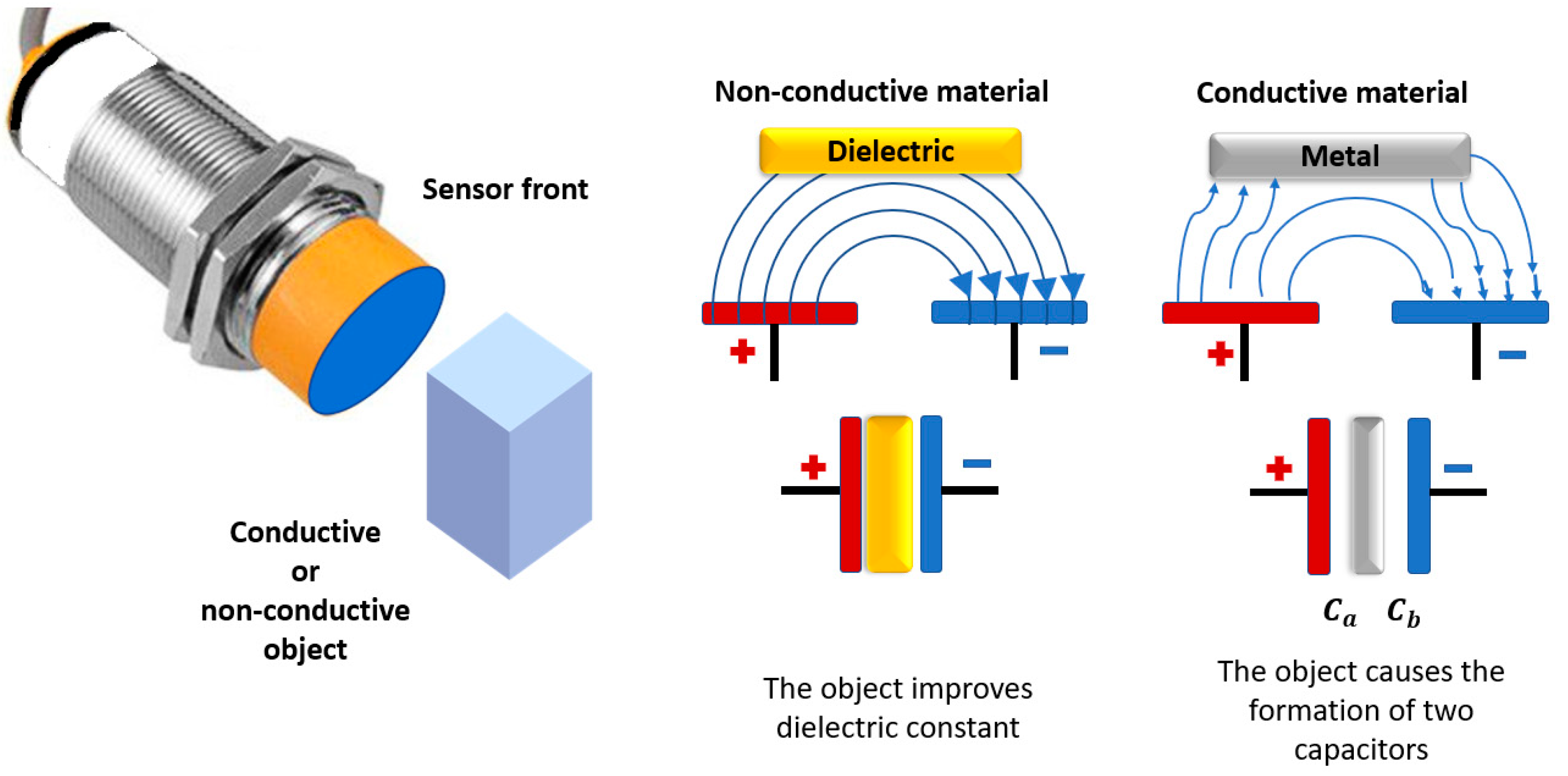
Figure 2.
Proposed diagram for the MT sensor
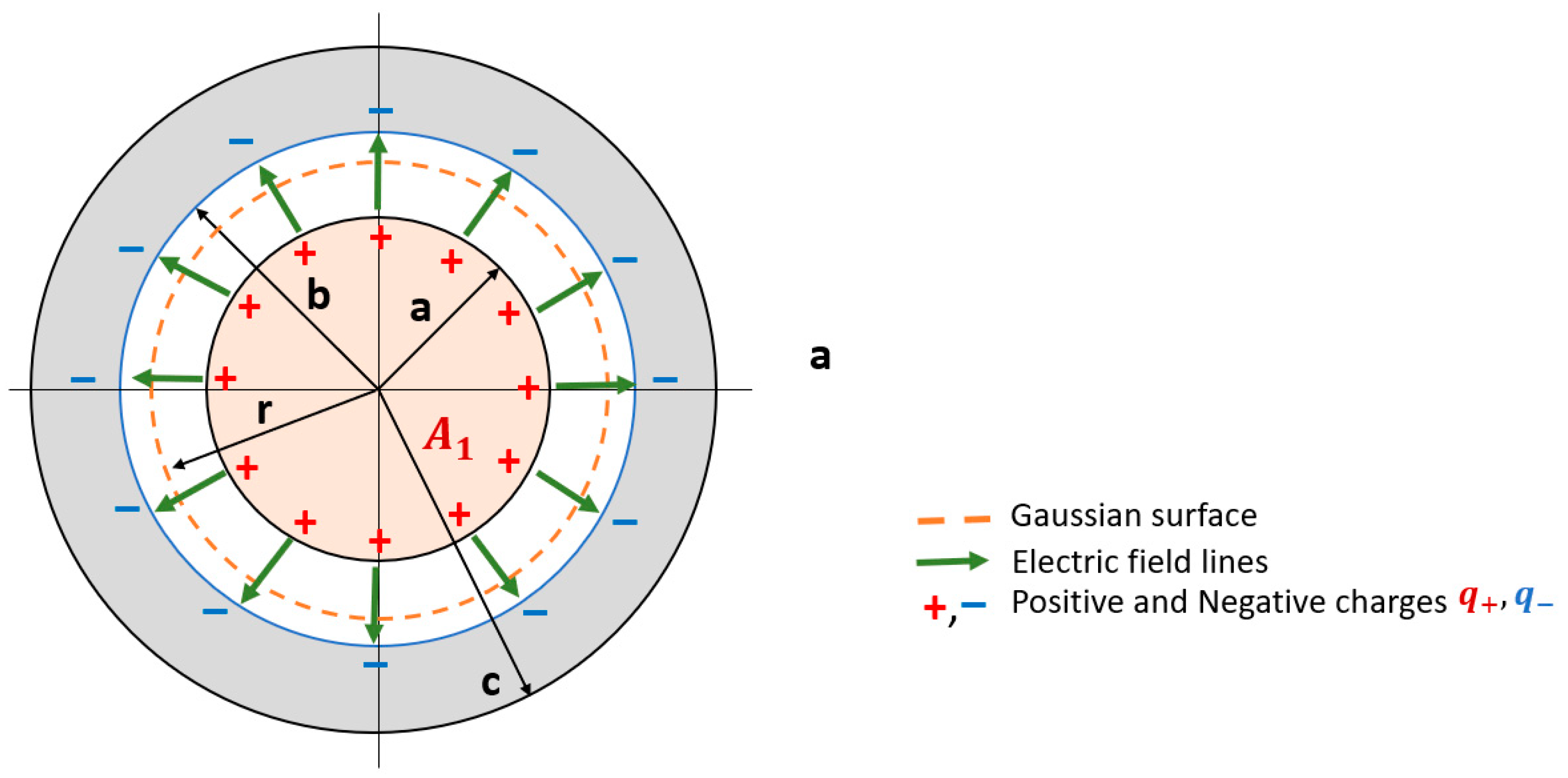
Figure 3.
Proposed diagram for the MNT sensor
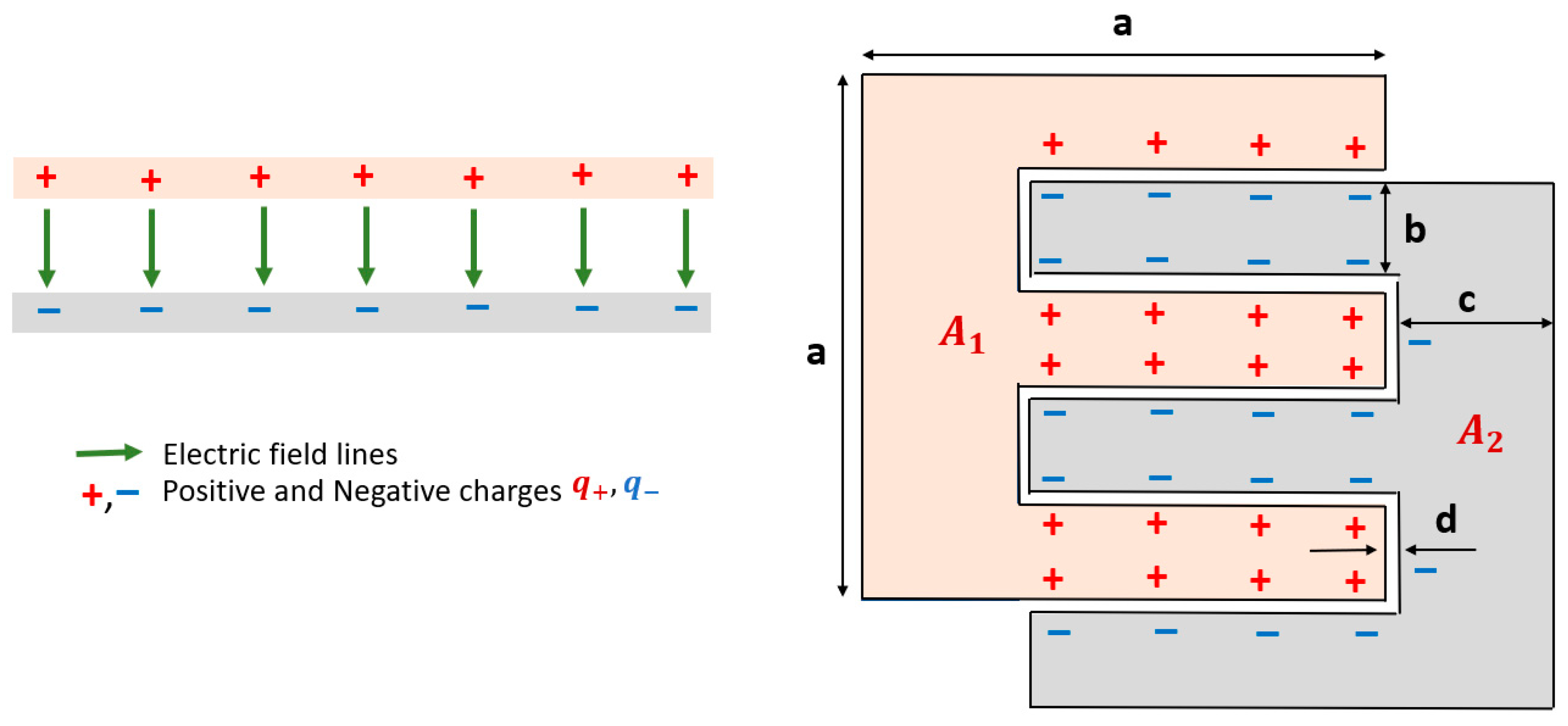
Figure 5.
Capacitance value with Non-Traditional Model Sensor Prototype (MNT) without residuals for reading.
Figure 5.
Capacitance value with Non-Traditional Model Sensor Prototype (MNT) without residuals for reading.
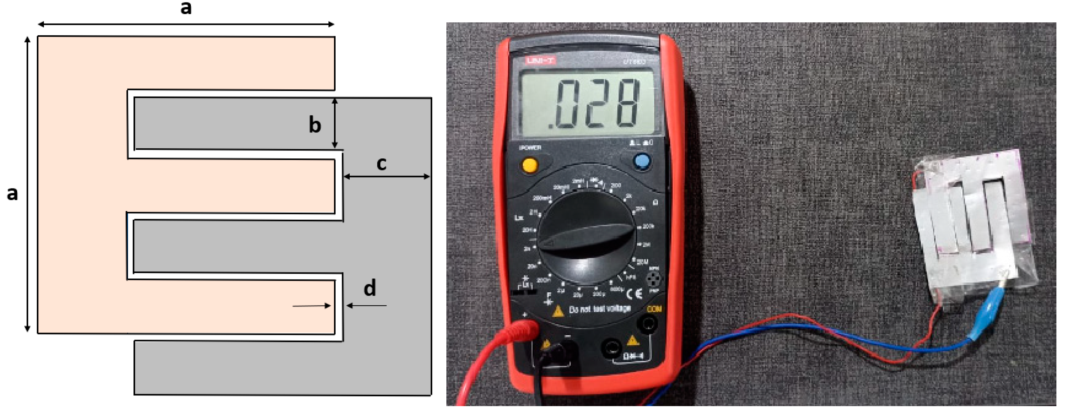
Table 1.
Electrical permittivity values for some types of plastic.
| Plastic Type | |
|---|---|
| Polyethylene | 2.3 |
| Polystyrene | 2.6 |
| Polypropylene | 2.2 a 2.6 |
| PVC | 2.9 |
| Polyethylene Terephthalate PET | 2.8 |
Disclaimer/Publisher’s Note: The statements, opinions and data contained in all publications are solely those of the individual author(s) and contributor(s) and not of MDPI and/or the editor(s). MDPI and/or the editor(s) disclaim responsibility for any injury to people or property resulting from any ideas, methods, instructions or products referred to in the content. |
© 2024 by the authors. Licensee MDPI, Basel, Switzerland. This article is an open access article distributed under the terms and conditions of the Creative Commons Attribution (CC BY) license (http://creativecommons.org/licenses/by/4.0/).
Copyright: This open access article is published under a Creative Commons CC BY 4.0 license, which permit the free download, distribution, and reuse, provided that the author and preprint are cited in any reuse.


