1. Introduction
Stormwater management has long been a key component of water resource planning, particularly in addressing nonpoint source pollution. In recent years, improving water quality has become central to these efforts, with a focus on evaluating Best Management Practices (BMPs) and seeking alternatives to overcome their limitations as regulations and standards evolve. Suspended sediments in stormwater are a major concern, as they often carry pollutants that adhere to these particles, posing a significant risk to water quality. Elevated levels of suspended sediment in receiving waterbodies threaten not only water quality but also aquatic ecosystems. Moreover, urbanization exacerbates these challenges through increased runoff, altered flow timing, and sediment deposition, further stressing the environment.
Nonpoint source pollution is widely dispersed runoff that carries contaminants and deposits them directly into natural waterbodies. Urban watersheds contribute a variety of pollutants, including oil, pesticides, nutrients, and sediment—essentially any contaminant found on the ground from both natural processes and human activities. Runoff from rainwater and snowmelt pick up these pollutants as they flow across different land uses within urban watersheds such as sidewalks, driveways, and parking lots, ultimately depositing them into streams as nonpoint source pollution. According to the United States Environmental Protection Agency (EPA), 46% of U.S. rivers and streams are in poor condition, primarily due to contamination from nutrients and sediment [
1]. Also, dissolved and suspended solids account for approximately 70% of total water pollution in urbanized areas [
2]. To address these issues, current EPA regulations mandate an 80% reduction in total suspended solids from urban runoff before it is discharged into waterways.
Traditional stormwater management practices have historically focused on water conveyance, prioritizing the rapid diversion of stormwater away from urban areas [
3]. However, the need to treat stormwater runoff has become increasingly recognized. This shift has driven the adoption of BMPs that target either contaminant-based or source-based treatment approaches [
4]. These BMPs have demonstrated their effectiveness in promoting natural flow paths, enhancing groundwater recharge, and preserving the aesthetic and environmental quality of urban areas, particularly through infiltration systems [
5]. Additionally, BMPs can be designed to serve multiple purposes, such as controlling floods and treating polluted runoff [
6]. By focusing on holistic benefits, BMPs for stormwater management can go beyond individual applications, providing broader advantages [
7]. For example, traditional BMPs such as detention ponds may not always be suitable in urban spaces due to their larger land requirements [
5]. Instead, enhanced BMPs should aim to retain and treat urban runoff on-site, utilizing strategies such as stormwater harvesting, detention or retention systems, and infiltration and biofiltration systems. These practices not only protect ecosystems but also contribute to long-term sustainability.
Bioswales are a type of BMP consisting of shallow, open-channel systems commonly used for managing stormwater and improving water quality, particularly by capturing and treating runoff from impervious surfaces such as roads and parking lots [
8]. When bioswales include an underdrain system, they are referred to as filtration BMPs; without an underdrain, they function as infiltration BMPs. These systems often feature dense vegetation, typically native plants, which slows down water flow, traps sediments, and removes pollutants [
9]. Bioswales are further classified into two types: wet swales (water treatment swales) and dry swales (grassed swales), depending on their specific applications [
10].
Dry swales are vegetated channels designed to capture and treat stormwater runoff, helping to meet both water quality and volume control objectives. Check dams or other barriers can be placed across the channel to promote water stagnation or ponding, which slows water flow, allowing pollutants to settle more easily [
8]. The reduced velocity also extends the hydraulic residence time (
HRT), facilitating gravitational settling and enhancing infiltration and evapotranspiration processes [
9,
10]. In bioswales with an underdrain system to aid infiltration, the goal is to limit ponding time to less than 48 hours. Additionally, the channel is typically designed to remain at least 2 ft (0.6 m) above the groundwater level, allowing the swale to function as a groundwater recharge facility. Dry swales are particularly effective at managing runoff from pollution “hotspots” and help prevent groundwater contamination, making them more suitable than wet swales for these applications [
8].
Wet swales function as shallow, channelized wetlands where wetland vegetation can be planted to trap pollutants as runoff flows through them [
11]. The water treatment processes in wet swales are primarily driven by thick vegetation that enhances filtration, flatter slopes that promote sedimentation, and nutrient uptake from the biomass present [
12]. While these processes make wet swales more effective at removing pollutants such as sediment, nutrients, nitrogen, and heavy metals [
13], their ability to mitigate peak stormwater runoff is limited, which constrains their broader application. Furthermore, the continuous presence of water in wet swales can pose challenges in urban environments, potentially interfering with existing infrastructure [
12]. Their larger footprint [
8] and the risk of mosquito breeding [
8,
11] also make wet swales less suitable for integration into urban landscapes.
The efficiency of infiltration-based treatment system, such as bioswales, is influenced by both runoff volume reduction [
14] and the types of pollutants present [
15]. Clark and Acomb (2008) [
16] noted that infiltrating runoff can help trap pollutants, promoting settlement and sedimentation. Coarser soils generally allow for faster water absorption due to higher infiltration rates compared to finer soils. Therefore, when designing stormwater infiltration systems, factors such as soil density and thickness are crucial [
17]. The infiltration capacity of the underlying soil directly affects the bioswale’s infiltration efficiency; however, bioswales are generally less effective at removing dissolved pollutants [
13,
18]. In some cases, treatment systems may even become sources of pollutants, such as total nitrogen [
19]. A study by King County in 1995 concluded that regular maintenance of treatment systems enhances their efficiency [
20].
To improve the performance of native soil, engineered media can be incorporated into bioswales [
17]. The gradation curve of the natural soil helps determine the specific requirements for soil amendments. If the natural soil has a particle size where
d10 > 0.02 mm and
d20 > 0.06 mm, indicating slower infiltration rates, soil amendment is recommended. The amendments, such as sand, gravel, or engineered materials, can enhance water quality, manage flooding, or serve both purposes [
10]. One notable option is expanded shale, a lightweight and porous material produced by firing clay or shale in a rotary kiln. Expanded shale improves drainage in clay soils—a common challenge in bioswales—and acts as a filter, enhancing water quality and pollutant removal [
21]. The study by Seters et al. (2006) [
22] found that bioswales significantly outperform asphalt pavement in removing common heavy metals like zinc and lead, though they may release higher nutrient levels. Additionally, research by Kim et al. (2003) [
23] demonstrated that introducing engineered media in bioretention systems can achieve 70-80% total nitrogen removal. Overall, the incorporation of engineered media in bioswale applications provides multiple advantages over native soil.
Expanded shale is available in various sizes, determined by its particle size distribution, which provides versatility for different applications. Manufacturers in North America produce expanded shale in size ranges such as 20-5 mm, 13-5 mm, and 10-2 mm. This material offers several beneficial characteristics, including a notably high specific surface area, low density, and exceptional durability, making it a resilient option for long-term use. Expanded shale has been utilized for multiple purposes, including improving soil drainage [
21,
24,
25], phosphorus removal and retention [
26,
27,
28], aeration for plant roots [
24], nitrogen removal [
29], and as a filter material in soil amendments [
30]. However, existing studies have not focused on the use of expanded shale in BMPs such as bioswales for water treatment purposes.
This study aims to evaluate the effectiveness of expanded shale in bioswales for stormwater treatment. The performance of dry swales enhanced with expanded shale was evaluated in a laboratory setting, considering variables such as soil media type and thickness, inflow rate, influent sediment concentration, and drainage conditions.
2. Materials and Methods
2.1. Experimental Setup
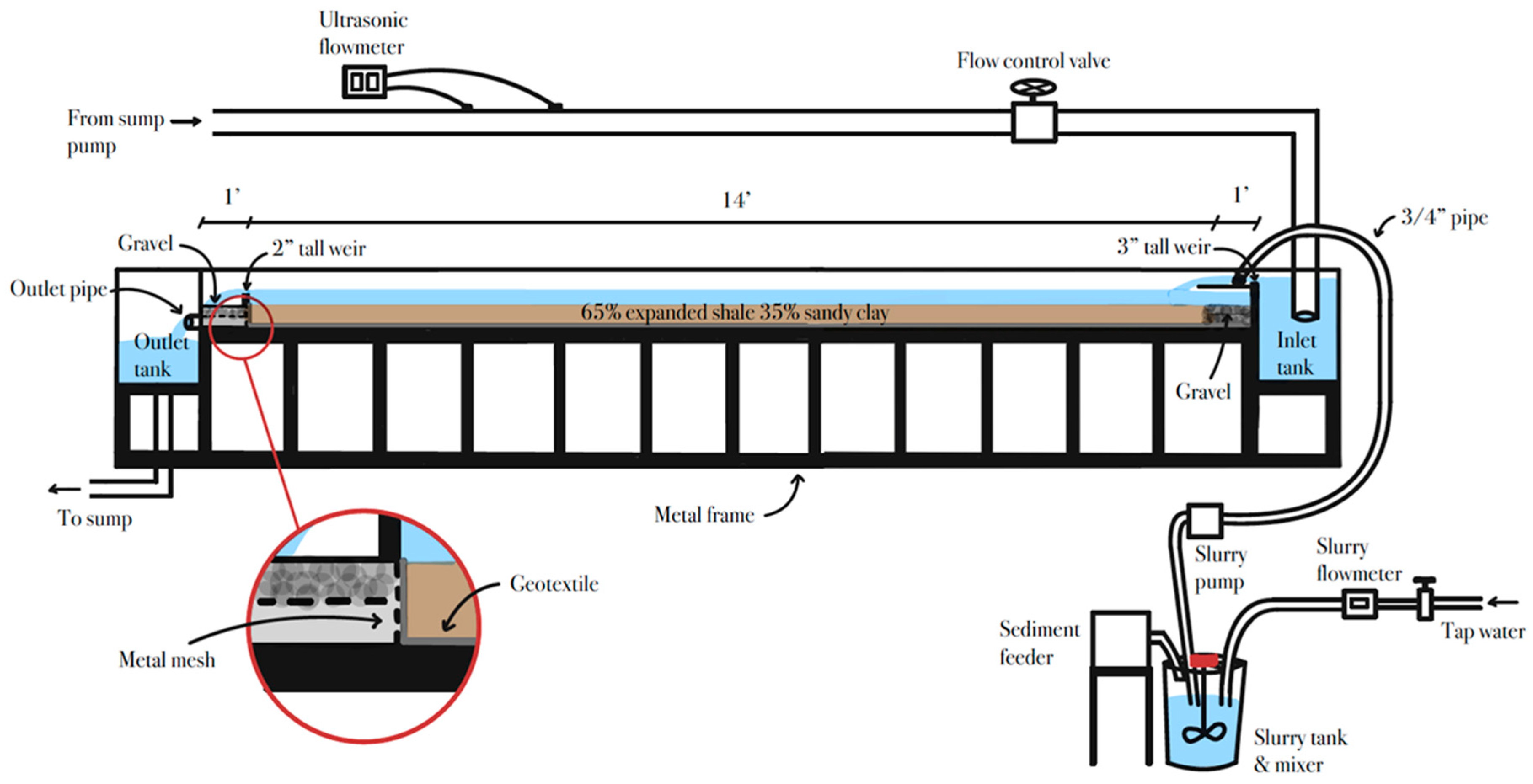
The experimental setup consisted of a plexiglass flume measuring 16 ft (4.9 m) long, 4 ft (1.2 m) wide, and 1.5 ft (0.45 m) deep, with inlet and outlet tanks attached at both ends. Each tank is 2 ft (0.6 m) long and 3 ft (0.9 m) deep, maintaining identical dimensions. Water enters the inlet tank through a 4-inch (10 cm) PVC inlet pipe, which features a perforated horizontal spreader at its base to ensure consistent water inflow. The outlet tank collects water that passes through the flume and redirects it back to the sump.
The flume is designed with an adjustable slope, set at 0.3% to comply with Caltrans’s recommendation of less than 1% for swales with underdrains [
10]. The engineered media, composed of 65% expanded shale and 35% sandy clay, was placed in the flume at two thicknesses: 6 inches (15 cm) and 4 inches (10 cm).
Figure 1 illustrates the experimental setup.
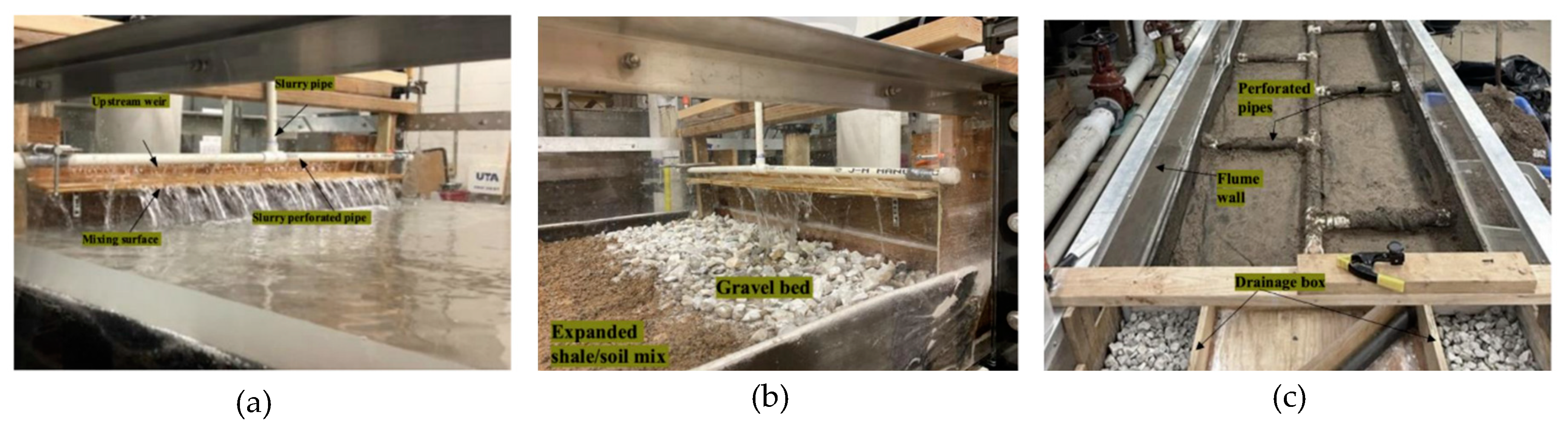
The experiments utilized two underground sumps to maintain a continuous water supply, which was regulated by a control valve on the 4-inch (10 cm) PVC inlet pipe. Flow rates were measured using a Sono-TraK ST30 ultrasonic flowmeter, with measurements verified through volumetric methods. A 3-inch (7.5 cm) high rectangular weir installed at the flume entrance ensured uniform flow distribution across the flume. A wooden plank placed downstream of the weir facilitated mixing of the sediment slurry with the inflow, which was introduced via a perforated pipe (
Figure 2a). Additionally, a layer of gravel at the flume’s entrance mitigated scouring (
Figure 2b). An underdrain system featuring 2-inch (5 cm) perforated pipes wrapped in geotextile was installed and controlled by a ball valve (
Figure 2c). A rectangular gravel-filled box with a 6-inch (15 cm) opening allowed for water flow, incorporating mesh and geotextile to retain soil. A perforated pipe within the box directed infiltrated water to the outlet tank. To regulate water depth over the soil media, a check dam was installed downstream of the flume, with a weir for overflow, ensuring a minimum water depth of 4 inches (10 cm) over the soil media (
Figure 1).
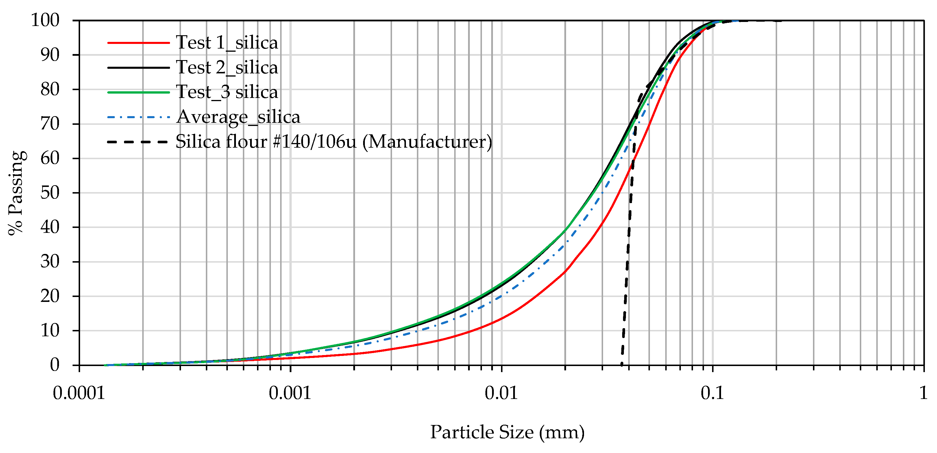
Silica flour #140/106u was used for the slurry, with its size gradation verified through three tests at the UTA Shimadzu Lab using a SALD-7101 nanoparticle size analyzer. The manufacturer’s gradations matched the UTA lab data for particles up to 0.037 mm in size but did not provide data for smaller particles (
Figure 3). Therefore, the lab data was used in the study. The selection of silica flour complied with the sediment particle size distribution requirements outlined by the New Jersey Department of Environmental Protection (NJDEP) [
31]. All sediment classes met or exceeded the minimum passing criteria, confirming the suitability of the silica flour to replicate suspended sediment loads typical of urban stormwater. Additionally, geotextile with a #80 size rating (0.18 mm opening) was used in conjunction with the engineered mix of expanded shale, which was more than 90% finer than 0.18 mm. The silica flour had a maximum particle size of 0.13 mm, ensuring that the geotextile would not trap influent particles and lead to clogging over time.
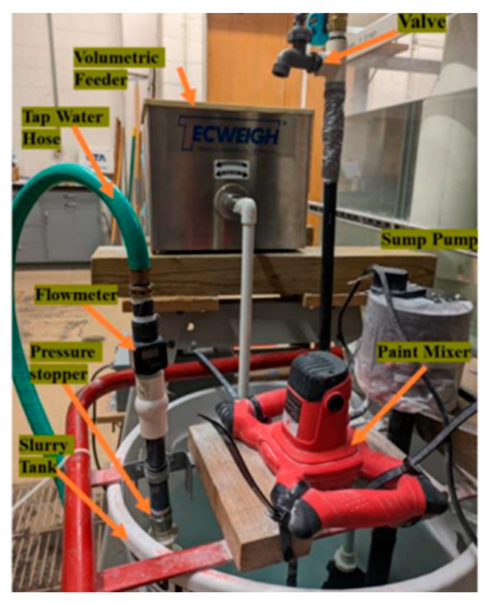
Silica flour and tap water were mixed in a cylindrical tank equipped with a mixer to maintain a uniform suspension and a float valve to regulate the water level in the tank. A flowmeter monitored water discharge into the mixing tank, while a volumetric sediment feeder controlled the injection of silica flour. A sump pump ensured consistent slurry flow into the flume, with a valve installed for sample collection to verify sediment concentration (
Figure 4). This setup provided a precise and constant rate of slurry entering the flume.
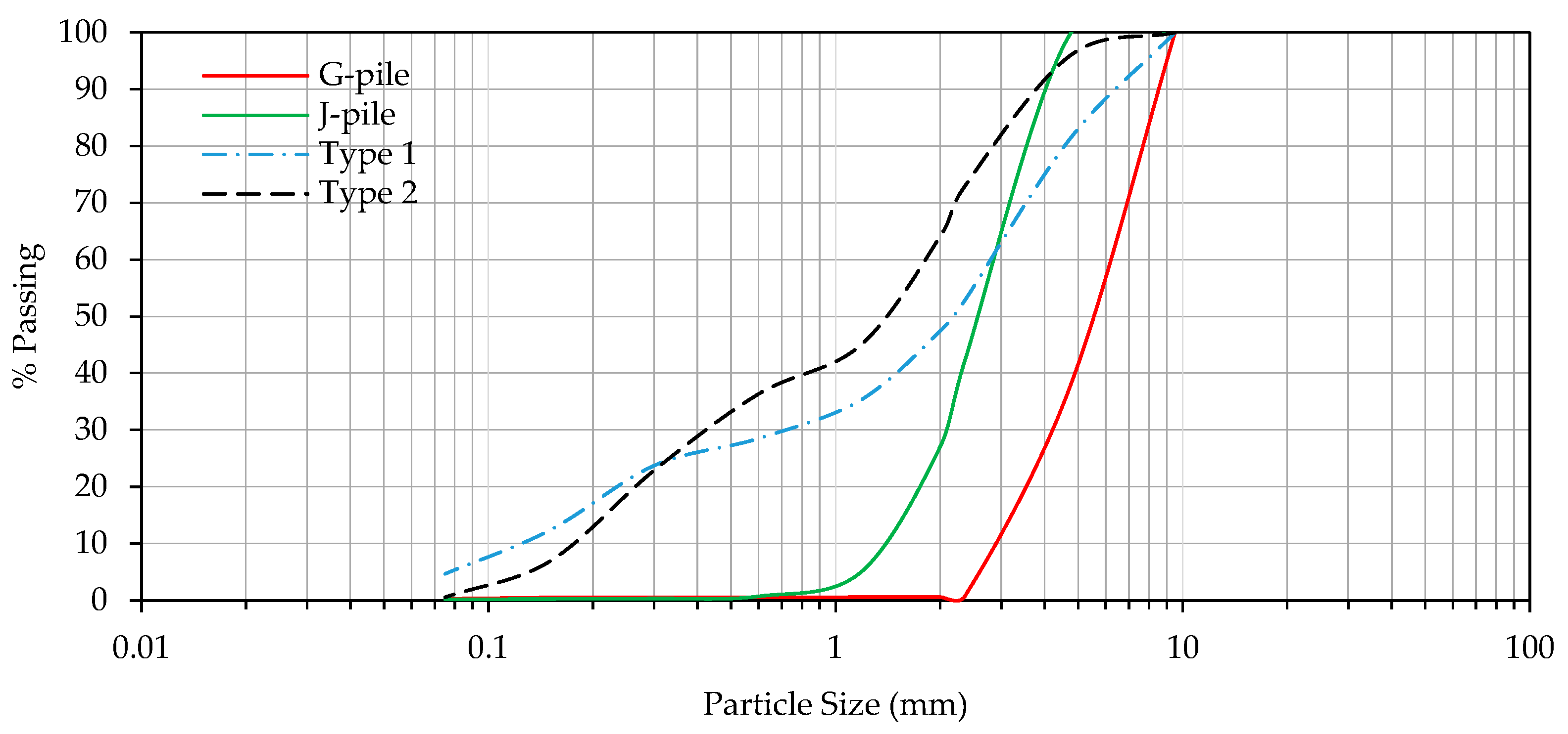
Two distinct filter media mixes were utilized in this investigation. Type 1 comprised a soil mix with a coarser expanded shale (medium size of ¾”), referred to as G-pile by the manufacturer. Conversely, Type 2 included a finer expanded shale with a median size of ¼”, labeled J-pile by the manufacturer. Both types maintained an identical composition of expanded shale and sandy clay, comprising 65% expanded shale and 35% natural sandy clay.
Sieve analysis tests were conducted for both types of expanded shale, G-pile and J-pile, as well as for the infiltration media prepared using these two types. All tests followed the ASTM-D6913 standard [
32].
Figure 5 presents the gradation curves obtained for G-pile and J-pile expanded shale, along with the Type-1 and Type-2 mixes.
A ball valve was used to control the underdrain system design. Close-valve setting limited the infiltration through the soil medium only, indicating the case without an underdrain configuration. Contrarywise, open-valve setting ensured the flow passed through both the soil medium and the underdrain pipe system, indicating the case of swales with an underdrain.
2.2. Inflow Rate and Influent Suspended Sediment Concentration
In the experiments, inflow rates were selected based on the design guidance for bioswales provided by Caltrans [
10]. The approach is based on meeting two criteria: a minimum hydraulic residence time (HRT) of 5 minutes for water treatment, and satisfying the interrelationship formula for water quality flow, as expressed by Equations 1 and 2.
where
V is the flow volume in ft
3 (m
3),
Q is the inflow rate in ft
3/s (m
3/s),
L is the channel length in ft (m),
v is the flow velocity in ft/s (m/s),
HRT is the hydraulic residence time in minutes,
is the depth for water quality flow in ft (m),
is the velocity for water quality flow in ft/s (m/s), and 60 is the unit conversion factor.
The maximum flow velocity was determined using Equation 1, based on the total length of the flume 16 ft (4.8 m), resulting in a velocity of 0.05 ft/s (0.015 m/s). Due to a downstream check dam in the flume, the flow depth was limited to 0.33 ft (11.4 cm). Using these parameters, the maximum water quality flow was calculated to be 0.066 ft³/s, equivalent to 112 Lit/min. Taking soil infiltration into account, a base flow rate of 120 Lit/min was selected. This flow rate corresponds to peak stormwater runoff from a 16,145 ft² (~1500 m²) drainage area experiencing a rainfall intensity of 0.5 in/hr (12.7 mm/hr), a commonly used value in stormwater treatment calculations [
33]. For the low flow scenario, a rate of 60 Lit/min was chosen based on recommendations from Claytor and Schueler (1996) for optimal filtration in water quality flows [
34]. Additionally, a high flow rate of 180 Lit/min was selected to remain within the allowable velocity limit, representing a peak flow scenario.
To represent a range of commonly reported suspended sediment concentrations in stormwater, influent concentrations of 100 mg/L and 200 mg/L were selected based on a literature review of highway runoff effluent [
33], ensuring coverage of both high and low suspended sediment concentration scenarios.
2.3. Drainage Capacity Tests
Before conducting the main test scenarios, drainage capacity tests were performed on the soil media. These tests involved measuring both overflow (flow passing over the downstream weir) and underflow (flow passing through the soil media and the drainage pipe) under various inflow rates and drainage conditions. The drainage capacity was estimated under with and without overflow conditions. To prevent overflow, the inflow rate was gradually increased while maintaining a flow depth of 4 inches (10 cm) in the flume, ensuring no spillover occurred. Volumetric flow measurements were performed using the EPA Bucket and Stopwatch method [
35]. Each flow measurement lasted for at least 10 seconds and was repeated three times for reliability. Additionally, the flow depth behind the downstream weir was recorded during experiments with overflow.
2.4. Experimental Procedure
A total of thirty experiments with varying parameters were conducted to evaluate factors influencing the reduction of total suspended solids (TSS) and turbidity. The study examined several variables, including inflow rate, thickness of soil media, underdrain conditions, influent sediment concentrations, and soil media type. Among these, twelve experiments utilized an active underdrain system (open-valve setting), while the remaining experiments did not (close-valve setting). Influent concentrations of 100 mg/L and 200 mg/L were tested, with soil media thickness of 4 inches (10 cm) and 6 inches (15 cm), except for Type 2 soil media, which was only tested at 4 inches (10 cm) due to poor performance observed with Type 1 soil mix at that thickness in reducing TSS and turbidity. Each experiment lasted at least 40 minutes to simulate typical rainfall duration and to comply with NJDEP recommended requirements [
31].
Table 1 summarizes the experiments conducted in the study.
Water samples for measuring TSS and turbidity were collected from various locations along and across the flume. For this study, a minimum hydraulic residence time (
HRT) of 8 minutes was required for low-flow scenarios. A sampling frequency of 10 minutes was selected, which satisfied the minimum
HRT criterion [
10].
Samples were collected from the slurry, inlet (after dilution), overflow, and underflow water. All samples were collected using the single-grab sample method as described by USGS (2006) [
36]. A clean 1-liter bottle, rinsed with distilled water, was quickly moved horizontally to collect a sample from the middle two-thirds of the flume width, minimizing boundary effects.
All samples underwent TSS and turbidity tests, except those from the intake (slurry tank), which were solely used for validation and quality assurance of targeted uniform mixing. Notably, turbidity testing was omitted for experiments 1 to 3 and all experiments involving 4-inch (10-cm) soil media due to logistical issues and their inferior performance compared to the 6-inch soil media.
Turbidity measurements were conducted using a Hach 2100Q portable turbidimeter, calibrated with standard samples of 20, 100, and 800 NTU, and verified with a 10 NTU standard, following EPA guidelines [
37]. TSS testing was performed according to EPA Method 160.2 [
38], which involved vigorous shaking and swirling of samples prior to testing. If TSS values were not within ±20% of the overall mean, samples were retested to ensure reliability.
TSS and turbidity testing were primarily conducted on the same day for all samples collected. When necessary, samples were stored at room temperature and tested within one day to avoid changes in sediment composition and concentration.
2.5. Particle Size Gradation Tests
A subset of water samples was analyzed for particle size gradation using a SALD-7101 nanoparticle size analyzer. This analysis aimed to determine the particle size distribution of both silica flour and selected water samples collected during the experiments. The procedure adhered to stringent protocols to maintain precision with the UV laser-equipped analyzer. Distilled water obtained from reverse osmosis was used to clean sampling bottles and, when necessary, to dilute samples. Prior to testing, dry silica flour was mixed with distilled water, and each sample underwent three evaluations to ensure consistency. The particle size analysis was conducted for experiments under high inflow (180 L/min) and low inflow (60 L/min) conditions. This assessment included samples from experiments involving various soil media types and influent sediment concentrations.
2.6. Calculation of Reduction in Total Suspended Solids and Turbidity
The efficiency of the soil media containing expanded shale in treating inflow sediment was evaluated by analyzing the TSS and turbidity data. This analysis involved calculating and comparing the weighted average reduction in TSS and turbidity, as described in Equation 3.
Equation 3 was also used to calculate the reduction in turbidity (Tu) by replacing TSS values with Tu in this equation.
2.7. Calculation of Swale Trap Efficiency
The Aberdeen equation (Equation 4), as utilized in similar research by Hunt et al. (2020) [
39], was employed to evaluate sediment trap efficiency based on only sedimentation processes within the swale. This equation estimates the expected efficiency of the swale. Due to its applicability in laminar flows, only the 60 L/min inflow rate was used for comparative purposes in this study. To calculate the expected efficiency using the Aberdeen equation, the Fall Number (
Nf)—which depends on the length of the channel (
L), settling velocity (
vs), flow velocity (
v), and flow depth (
d)—was applied.
The study also incorporated particle size distribution (PSD) analysis to calculate the weighted average trap efficiency of the sediment used in the experiments. This efficiency, based on PSD, was compared with the efficiencies calculated using the median diameter (d50) of sediment gradation at the flume inlet.
Lastly, the theoretical required length of the flume to achieve 80% suspended sediment removal, solely through particle settling, was determined using the Aberdeen equation. The trapping efficiency was calculated for various hypothetical flume lengths and compared as per the Aberdeen equation (Equation 4).
4. Discussion
This study aimed to evaluate the effectiveness of expanded shale as an infiltration medium in bioswales for stormwater runoff treatment. Laboratory experiments were conducted under varying conditions, including different soil media thicknesses and gradations, flow rates, and influent sediment concentration to assess the material’s performance in removing pollutants such as suspended sediment. Continuous monitoring of inflow and outflow, along with water quality analysis, provided key insights into the efficiency of expanded shale.
The findings indicated that when an underdrain system was present, both coarse and fine media exhibited similar infiltration rates. However, in experiments without an underdrain, coarser media showed a higher infiltration rate under zero overflow conditions. This observation is consistent with the Minnesota Pollution Control Agency’s assertion that soil characteristics influence infiltration rates, with coarser soils generally allowing faster infiltration [
17].
Increasing the thickness of the soil media to 6 inches (15 cm) consistently improved TSS reduction along the entire channel length, compared to the 4-inch (10-cm) layer. This suggests that a thicker layer of expanded shale is more effective at removing sediment, supporting previous research [
40,
41], which highlights the benefits of thicker infiltration layers for pollutant and volume reduction.
In scenarios with an active underdrain system, coarser expanded shale generally performed better than finer media, whereas the performance of both media types was similar when the underdrain was inactive. The active underdrain enhanced pollutant removal efficiency by improving drainage and increasing contact time between water and the shale, thus facilitating greater adsorption. This finding aligns with previous studies that underscore the importance of infiltration for effective pollutant removal [
15,
16]. Incorporating water storage mechanisms in bioswales can significantly boost pollutant removal by trapping stormwater longer and enhancing nutrient removal [
40]. Therefore, integrating underdrain systems and ponding mechanisms into bioswale design can improve stormwater treatment and water quality outcomes.
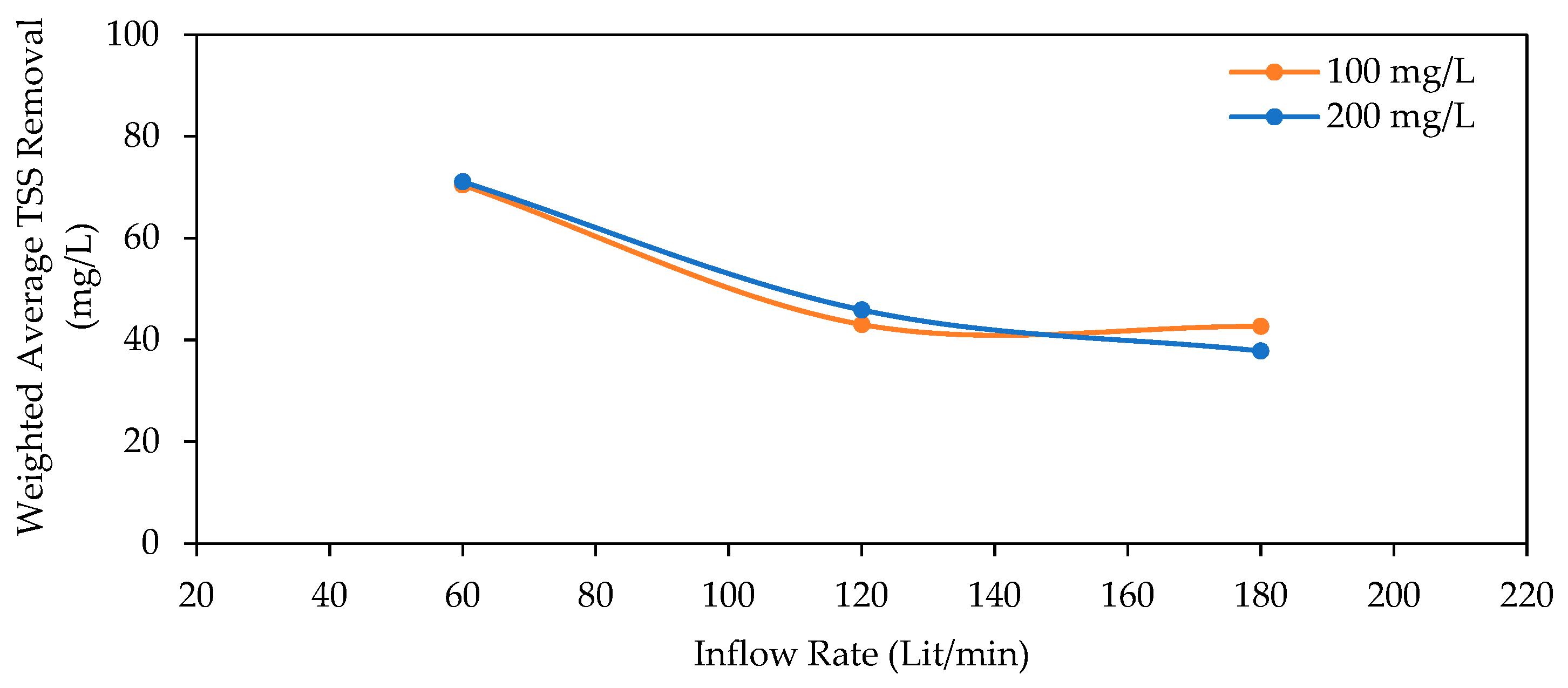
The study revealed that as inflow rates increased, the efficiency of TSS and turbidity removal decreased, demonstrating the need to account for inflow rate variations when developing stormwater management strategies. Similar trends have been reported for TSS and turbidity removal in bioswales, highlighting the critical link between pollutant removal efficiency and flow rates [
42]. These results emphasize the importance of incorporating flow rate variability into stormwater management planning to optimize pollutant removal.
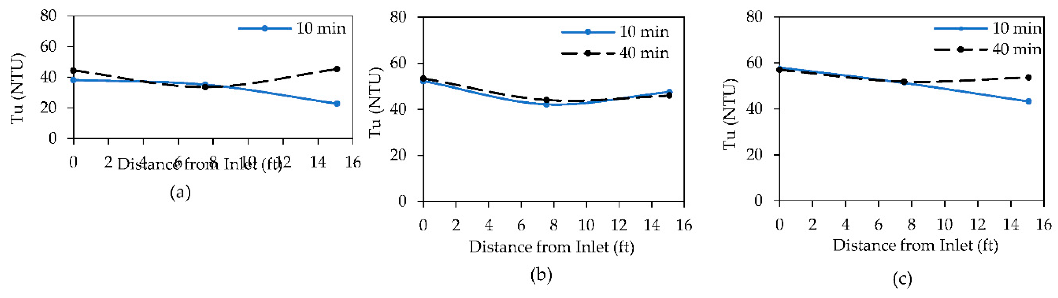
While reductions in TSS and turbidity were observed in most scenarios, the bioswale was less effective at reducing turbidity, with some cases showing increased turbidity in the middle section of the flume and in overflow samples. This increase could be due to sediment resuspension, possibly caused by the presence of check dams, or the changing composition of suspended sediment, resulting in finer particles along the flow. Higher turbidity in overflow samples compared to infiltrated water has been previously reported in bioswale studies [
43].
The study also found that while TSS and turbidity reductions were generally similar for both low and high influent sediment concentrations, some individual experiments showed differences in TSS removal in outflow (infiltrated water). Doubling the influent concentration from 100 to 200 mg/L resulted in a corresponding doubling of the effluent concentration range, indicating that bioswale efficiency is influenced by the initial sediment load [
33].
A more rapid reduction in TSS was observed in the first half of the flume, followed by a slower reduction in the second half. This pattern is consistent with previous research showing an exponential decrease in TSS concentration along the flow path [
41,
44].
Particle size gradation analysis revealed distinct sediment behavior in the swale. During low inflow scenarios, coarser particles predominantly settled in the upstream section, resulting in significant reductions in TSS and turbidity in the first half of the swale. This settling trend remained stable over time. However, under high inflow conditions, increased flow velocity shortened hydraulic residence time, preventing adequate settling of coarser particles. As a result, coarser particles were found in the overflow, contrasting with low inflow scenarios where finer particles were more prevalent. The particle size distribution was notably influenced in the middle section and overflow regions by variations in flow rates, underscoring the role of flow dynamics in sediment transport. Unlike low inflow experiments, where particle size noticeably decreased along the swale, high inflow experiments showed minimal variation in particle size distribution. These results align with prior studies, suggesting a consistent pattern of sediment size reduction during low inflows.
Overall, this study highlights the importance of considering flow dynamics in sediment transport processes within bioswales for effective water quality management.
5. Conclusions
Bioswales, commonly employed as BMPs, are designed to enhance water quality and manage peak flows during extreme storm events. The efficiency of these BMPs is primarily evaluated based on their ability to reduce pollutants in stormwater. While conventional filter media such as rocks, sand, and mulch have been widely used to improve infiltration in bioswales, the potential of engineered expanded shale as an alternative medium remains relatively underexplored and lacks comprehensive documentation.
The main objective of this study was to assess the treatment effectiveness of expanded shale when used as an infiltration medium in bioswales. Initially, the study focused on determining how the thickness of the infiltration media influences sediment removal efficiency. Following this, the chosen thickness of expanded shale was tested under various conditions, including differences in soil media properties, inflow rates, influent concentrations, and drainage configurations. Additionally, the study investigated changes in sediment particle size along the length of the bioswale channel to further understand its filtration dynamics.
The findings from thirty laboratory experiments and gradation analysis, demonstrated that using expanded shale in bioswales resulted in sediment removal efficiencies ranging from 20% to 82% for TSS, and a variable range of -4% to 61% for turbidity under different conditions. The results indicated that expanded shale performed more efficiently than other filtration materials such as sand and gravel and required significantly less channel length compared to typical bioswale applications. Remarkably, even in a small-scale laboratory model, expanded shale achieved sediment removal standards of 80%, and more in some scenarios meeting current regulatory requirements.
The results of this study showed that expanded shale offers additional advantages for bioswales, including superior drainage that helps prevent clogging. Its large surface area promotes pollutant removal, enhancing treatment efficiency. Combining expanded shale with underdrain systems further improves drainage efficiency, while geofabrics can help prevent fine particles from clogging underdrains, thus ensuring the long-term functionality of the bioswale.
In conclusion, expanded shale is a highly effective filtration medium for bioswale applications, offering substantial improvements in stormwater management. This study provides a foundation for further research and practical applications, emphasizing the need for customized bioswale designs to enhance water quality management in urban settings. Future research can expand upon these findings by focusing on several key areas:
Comprehensive field experiments: Real-world field studies are necessary to more accurately assess the efficiency of expanded shale under actual stormwater conditions.
Clogging impact: Investigating the long-term effects of clogging on expanded shale’s performance and developing mitigation strategies will be critical.
Inflow patterns: Studying diverse inflow patterns, including lateral flows, will help to better understand how different flow dynamics influence expanded shale-based systems.
Vegetation influences: Exploring the interaction between vegetation and expanded shale could lead to optimized designs that enhance stormwater management.
Cost-benefit analysis: Conducting economic evaluations comparing expanded shale to traditional filter media can help assess its financial feasibility.
By addressing these areas, future research can enhance the understanding and application of expanded shale in stormwater management, fostering more sustainable urban water practices.
Figure 1.
Schematic diagram of the experimental setup (not to scale).
Figure 1.
Schematic diagram of the experimental setup (not to scale).
Figure 2.
(a) Inlet configuration of the flume setup showing inlet weir, slurry perforated pipe, and mixing surface, (b) Gravel bed installed to prevent scour, and (c) Underdrain system integrated within the soil medium, along with the outlet drainage box.
Figure 2.
(a) Inlet configuration of the flume setup showing inlet weir, slurry perforated pipe, and mixing surface, (b) Gravel bed installed to prevent scour, and (c) Underdrain system integrated within the soil medium, along with the outlet drainage box.
Figure 3.
Particle size gradation curves of silica flour used in slurry.
Figure 3.
Particle size gradation curves of silica flour used in slurry.
Figure 4.
Sediment feeder and slurry tank set up.
Figure 4.
Sediment feeder and slurry tank set up.
Figure 5.
Particle size gradation curves of the coarse and fine expanded shale (G-pile and J-pile), and Type 1 and Type 2 media prepared using these two materials.
Figure 5.
Particle size gradation curves of the coarse and fine expanded shale (G-pile and J-pile), and Type 1 and Type 2 media prepared using these two materials.
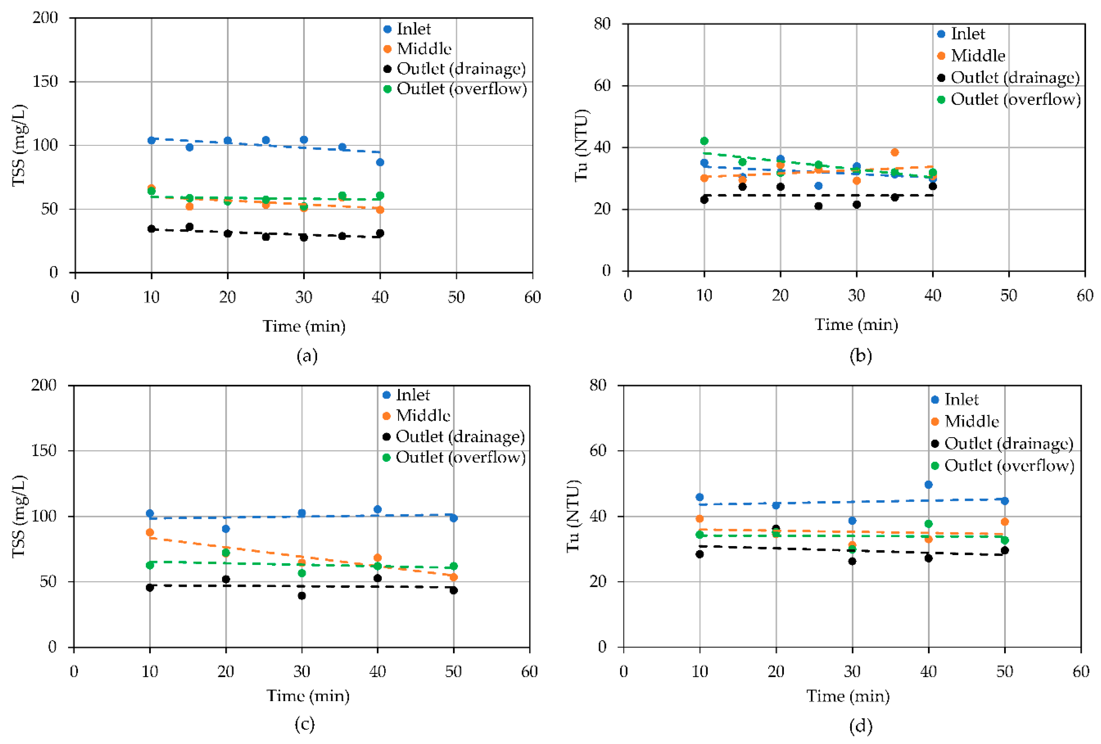
Figure 6.
TSS and turbidity variation at inlet, middle section, underflow (drainae), and overflow in the experiment with inflow rate of 120 Lit/min, influent sediment concentration of 100 mg/L, and soil media of 6-inch (15-cm) thickness (a,b), and 4-inch (10-cm) thickness (c, d).
Figure 6.
TSS and turbidity variation at inlet, middle section, underflow (drainae), and overflow in the experiment with inflow rate of 120 Lit/min, influent sediment concentration of 100 mg/L, and soil media of 6-inch (15-cm) thickness (a,b), and 4-inch (10-cm) thickness (c, d).
Figure 7.
Weighted average TSS removal under different inflow rates and sediment loading.
Figure 7.
Weighted average TSS removal under different inflow rates and sediment loading.
Figure 8.
Variation in turbidity along the flume (at various sampling locations) at different times in experiments with inflow rates of: (a) 60 Lit/min, (b) 120 Lit/min, and (c) 180 Lit/min.
Figure 8.
Variation in turbidity along the flume (at various sampling locations) at different times in experiments with inflow rates of: (a) 60 Lit/min, (b) 120 Lit/min, and (c) 180 Lit/min.
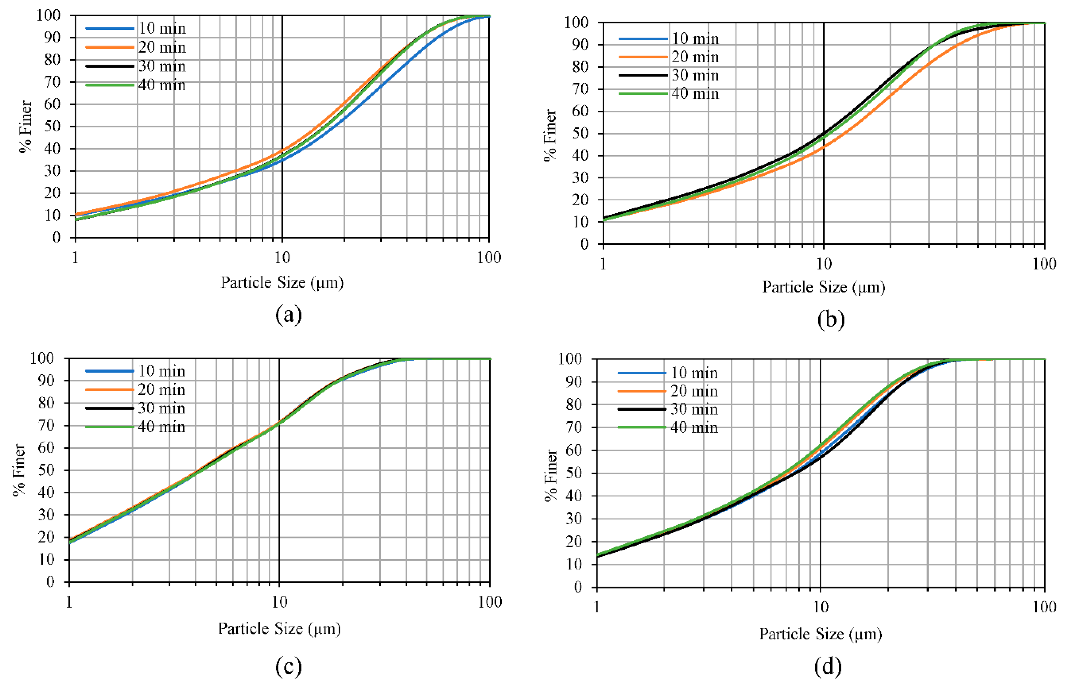
Figure 9.
Changes in suspended sediment gradation with time at (a) Inlet, (b) Middle section, (c) Underflow, and (d) Overflow (Type 2 media, inflow rate 180 Lit/min, influent sediment concentration 100 mg/L).
Figure 9.
Changes in suspended sediment gradation with time at (a) Inlet, (b) Middle section, (c) Underflow, and (d) Overflow (Type 2 media, inflow rate 180 Lit/min, influent sediment concentration 100 mg/L).
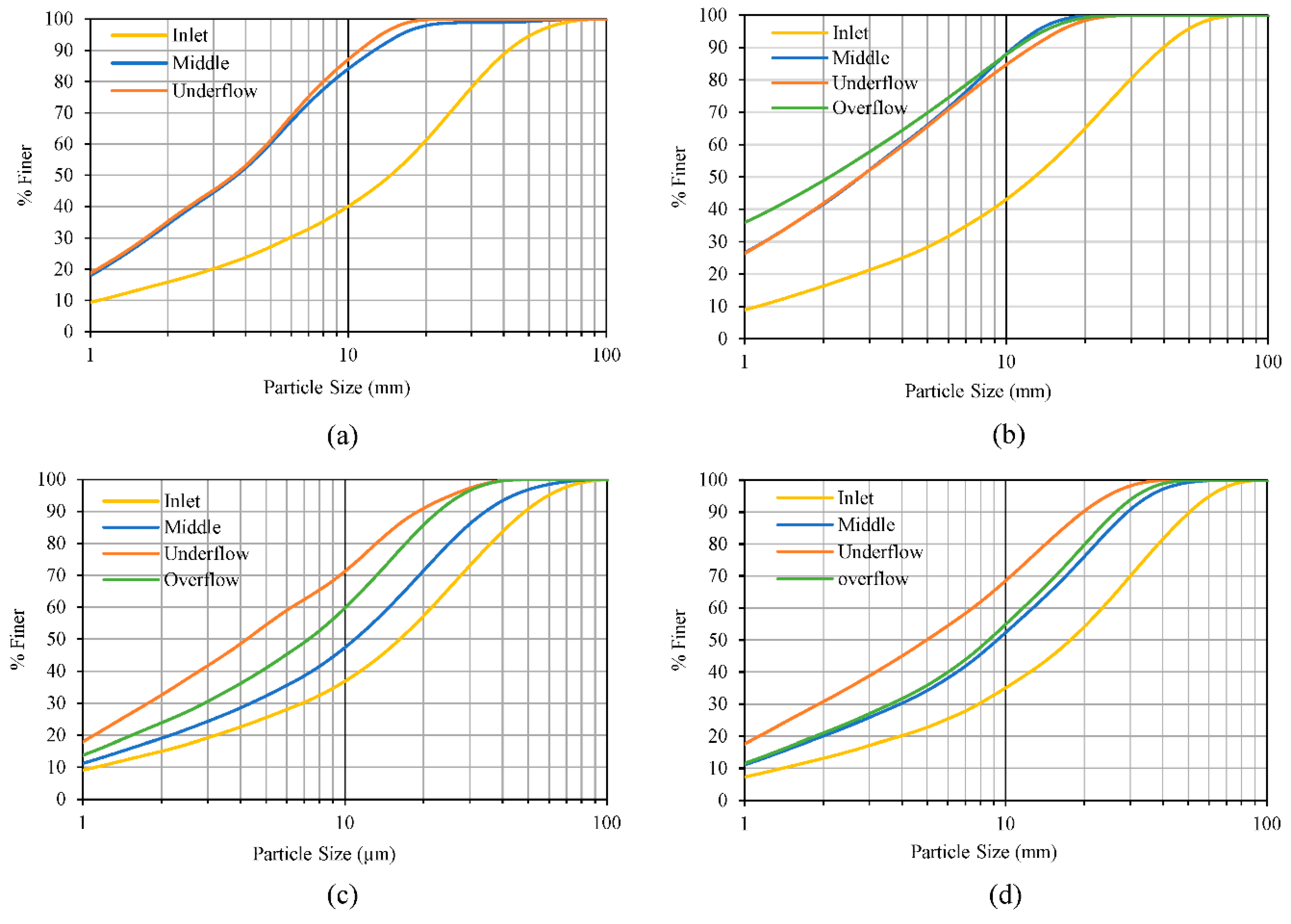
Figure 10.
Changes in suspended sediment gradation with inflow rate and influent concentration of: (a) 60 Lit/min, 100 mg/L (note: since there was no overflow in this experiment, the gradation curve is not prepared), (b) 60 Lit/min, 200 mg/L, (c) 180 Lit/min, 100 mg/L, and (d) 180 Lit/min, 200 mg/L.
Figure 11.
Trap efficiency vs swale required length using Aberdeen Equation.
Figure 11.
Trap efficiency vs swale required length using Aberdeen Equation.
Table 1.
Summary of Experiment Scenarios.
Table 1.
Summary of Experiment Scenarios.
| Experiment No. |
Infiltration Media |
Media Thickness (inches) |
Drainage Condition |
Inflow
(L/min) |
Influent Sediment
Concentrations (mg/Lit) |
| 1 |
Type 1: Coarse Media |
6 |
Open-valve |
60 |
100 |
| 2 |
120 |
| 3 |
180 |
| 4 |
60 |
200 |
| 5 |
120 |
| 6 |
180 |
| 7 |
Close-valve |
60 |
100 |
| 8 |
120 |
| 9 |
180 |
| 10 |
60 |
200 |
| 11 |
120 |
| 12 |
180 |
| 13 |
4 |
Close-valve |
60 |
100 |
| 14 |
120 |
| 15 |
180 |
| 16 |
60 |
200 |
| 17 |
120 |
| 18 |
180 |
| 19 |
Type 2: Fine Media |
6 |
Open-valve |
60 |
100 |
| 20 |
120 |
| 21 |
180 |
| 22 |
60 |
200 |
| 23 |
120 |
| 24 |
180 |
| 25 |
Close-valve |
60 |
100 |
| 26 |
120 |
| 27 |
180 |
| 28 |
60 |
200 |
| 29 |
120 |
| 30 |
180 |
Table 2.
Drainage Capacity of Type 1 and Type 2 Soil Media (without underdrain).
Table 2.
Drainage Capacity of Type 1 and Type 2 Soil Media (without underdrain).
Media
Type |
Target Inflow
(Lit/min) |
Actual Inflow
(Lit/min) |
Underflow
(Lit/min) |
Overflow
(Lit/min) |
Water Depth
(cm) |
| Type 1 |
- |
46.2 |
46.2 |
- |
10.0 |
| 60 |
59.5 |
48 |
11.5 |
10.06 |
| 120 |
120.2 |
53.4 |
66.8 |
10.38 |
| 180 |
182.2 |
55.2 |
127 |
10.69 |
| Type 2 |
- |
41.2 |
41.2 |
- |
10.0 |
| 60 |
62.1 |
42 |
20.1 |
10.06 |
| 120 |
120.2 |
43.8 |
76.4 |
10.5 |
| 180 |
182.2 |
48 |
134.2 |
10.75 |
Table 3.
Drainage Capacity of Type 1 and Type 2 Soil Media (with underdrain).
Table 3.
Drainage Capacity of Type 1 and Type 2 Soil Media (with underdrain).
Media
Type |
Target Inflow
(Lit/min) |
Actual Inflow
(Lit/min) |
Underflow
(Lit/min) |
Overflow
(Lit/min) |
Water Depth
(cm) |
| Type 1 |
60 |
60.7 |
60.7 |
- |
10.0 |
| - |
66.5 |
66.5 |
- |
10.0 |
| 120 |
120.2 |
68.4 |
51.8 |
51.8 |
| 180 |
182.2 |
72 |
110.2 |
110.2 |
| Type 2 |
60 |
60.7 |
60.7 |
- |
10.0 |
| - |
70.6 |
65.4 |
5.2 |
10.0 |
| 120 |
120.2 |
71.4 |
48.8 |
10.25 |
| 180 |
185.2 |
72.6 |
112.6 |
10.63 |
Table 4.
Weighted Average TSS Removal of Similar Experiments with Different Soil Media Thickness.
Table 4.
Weighted Average TSS Removal of Similar Experiments with Different Soil Media Thickness.
| Media Type |
Weighted Average TSS Removal (%) |
| 60 Lit/min |
120 Lit/min |
180 Lit/min |
| 4-inch media |
56 |
40 |
33 |
| 6-inch media |
66 |
42 |
36 |
Table 5.
Weighted Average TSS Removal of Similar Experiments with Different Soil Media Types and Drainage Conditions.
Table 5.
Weighted Average TSS Removal of Similar Experiments with Different Soil Media Types and Drainage Conditions.
| Media Type/Drainage Condition |
Weighted Average TSS Removal (%) |
| 60 Lit/min |
120 Lit/min |
180 Lit/min |
| Type 1 |
72 |
47 |
41 |
| Type 2 |
70 |
42 |
39 |
| Without underdrain |
66 |
42 |
34 |
| With underdrain |
76 |
47 |
47 |
Table 6.
Average and Range of TSS Removal at Various Sampling Locations.
Table 6.
Average and Range of TSS Removal at Various Sampling Locations.
| Location |
Mean TSS Removal (%) |
Range of TSS Removal (%) |
| Half of Swale Length |
42 |
20 - 75 |
| Overflow |
63 |
19 - 75 |
| Underflow |
68 |
55 - 82 |
| Mean* |
52 |
30 - 82 |
Table 7.
Swale Trap Efficiency based on PSD and d50 and Required Swale Length for 80% TSS Reduction using Aberdeen Equation.
Table 7.
Swale Trap Efficiency based on PSD and d50 and Required Swale Length for 80% TSS Reduction using Aberdeen Equation.
| Overflow (Lit/min) |
Flume Width (m) |
Velocity
(m/s) |
HRT (min) |
Method of Calculation |
Calculated Trap Efficiency (%) |
Observed Trap Efficiency (%) |
| Full Length |
Half
Length |
Full Length |
Half Length |
| 44 |
1.22 |
0.006 |
8.81 |
Based on d50
|
19.6 |
13.1 |
71 |
75 |
| Based on PSD |
21.5 |
15.7 |