
Submitted:
22 November 2024
Posted:
25 November 2024
You are already at the latest version
Abstract
Urban landscapes are highly heterogeneous but possess recurrent, distinguishable features known as urban landscape types, which exhibit distinct social and environmental performance, and collectively form an urban landscape typology (ULT). ULT is useful as they can aid decision-making in urban planning, predicting the impact of various development proposals. Past attempts to develop ULT overlooked important land features including land use. We developed a conceptual framework based upon the recent literature, and operationalized it using Singapore, an archetypical compact city. Fourteen geospatial variables representing five main components of urban landscapes (land cover composition and configuration, land use, building density, and elevation) were used in a heuristic process to construct a series of models using varying clustering algorithms, coupled with adjustments utilizing contextual knowledge. Models were then tested for their performance regarding practical and environmental relevance. Our results identify ten distinguishable landscape types in Singapore. The six variables that were used in characterizing the UTL were: percent impervious surface, land cover diversity, land use diversity, building density, elevation, and percent water. Initial inspection against Google Earth, followed by a systematic validation exercise by urban planning and design students and professionals confirmed that the ten landscape types adequately correspond to distinguishable urban forms. The ULT were also examined for their ability to estimate land surface temperature (LST) as an environmental performance example; our results demonstrated that all landscape types had significantly different LSTs. We believe that our ULT and the methodological approach we adopted can assist in integrating urban ecological knowledge into practice.
Keywords:
urban landscape typology
; urban form
; urban ecology
; urban planning
; urban design
; compact city
; environmental remote sensing
1. Introduction
Urban landscapes are highly heterogeneous and refer to a subset of the larger human-dominated ecosystems, which are shaped by the complex interplay between natural and social factors and are experienced by people (Tan et al., 2018). They consist of physical urban elements, such as transport and drainage infrastructure, buildings, vegetated areas, open spaces, etc., intertwined with socio-economic and ecological networks that are non-physical in nature (Tan et al., 2018). The physical forms of urban landscapes manifest in markedly varied urban morphological patterns, such as compact versus sprawling, low-rise versus high-rise, concentric versus grid, each of which can have correspondingly differentiated patterns of arrangement of natural and semi-natural ecosystems. These varied morphological patterns are expected to influence the flow of materials, people, information and energy across an urban area which in turn, affect its ecological, social and environmental conditions (Forman, 2014). This is analogous to a principal tenet in landscape ecology—that there is spatial association between the spatial pattern of landscape elements and ecological processes and functions in a given landscape (Forman, 2014; Forman & Godron, 1986; Turner, 1989).
Spatial pattern in this context is defined as type and abundance of different landscape elements (patches) and their spatial character and arrangement, such as geometrical shape complexity and the fragmentation level (McGarigal & Marks, 1995). Emerging but scattered evidence confirms the influence landscape pattern has on key ecological and social functions of urban areas. For instance, areas with higher amounts of vegetation exhibit cooler temperatures, more stormwater absorption and a variety of health benefits compared to less vegetated regions (Pataki et al., 2021). More connected and less fragmented pattern of urban green spaces exhibited lower land surface temperatures (Masoudi & Tan, 2019). More densely built-up urban areas have been shown to suffer from more stormwater runoff (Tratalos et al., 2007). Patches of secondary forests are more effective in cooling the surrounding environment than managed trees (Richards et al., 2020). A meta-analysis of 62 studies showed that a scattered pattern of trees could promote higher levels of biodiversity (Prevedello et al., 2017). Green space morphology also exert effects on human mortality (Wang & Tassinary, 2019). As knowledge continues to grow in this area, we suggest that a possible approach to augment our knowledge of pattern-function relationships is to understand and develop improved methods for classifying urban landscape patterns.
Despite the high level of heterogeneity and complexity of urban landscapes, it is possible to identify areas that are homogeneous enough to form discrete units of landscape at certain scales that are repeated and recognisable across the city. In other words, “finding homogeneity in heterogeneity” (Messerli et al., 2009). Such landscape units may be referred to as a “landscape typology” and defined as “a systematic classification of landscape types based on attributes that describe properties of interest” (Van Eetvelde & Antrop, 2009). We adopt the concept of landscape typology for urban landscapes and refer to it as the “urban landscape typology” (ULT) in the remainder of the paper. Many attempts have been made to develop ULT, from the early works by (Anderson et al., 1976) and (Ridd, 1995), to more recent typology systems such as the High Ecological Resolution Classification for Urban Landscapes and Environmental Systems (HERCULES) (Cadenasso et al., 2007), Local Climate Zones (LCZ) (Stewart & Oke, 2012), and Structure of Urban Landscapes (STURLA) (Hamstead et al., 2016). The produced ULTs are different depending on the origin of the landscape concept—whether or not it is based on natural or social sciences—the level of objectivity and user intervention, and the objectives of the typological system (Simensen et al., 2018).
Early ULTs were mostly based on aggregate categories of land cover and land use, and over time increasing attention was paid to other elements of the urban ecosystem, such as building height (Cadenasso et al., 2007) and spatial pattern of land cover (Mücher et al., 2010) This trend can be explained by two main reasons: 1) it has become feasible to include more information due to the advancements in remote sensing and geospatial technologies, and 2) it has become increasingly clear that landscape elements other than land cover and land use affect ecological and environmental processes. As a result, recently developed typologies are more complex and attempt to better reflect the true nature of urban landscapes as highly complex social-ecological-technological systems (Hamstead et al., 2016).
Given the relationship between pattern and ecological and environmental processes and functions (Alberti, 2007; Forman, 2014), different landscape types are expected to have differential environmental performance as also demonstrated by previous studies that have tested the suitability of their ULTs against temperature in different cities (Bechtel et al., 2019; Hamstead et al., 2016; Larondelle, Hamstead, Kremer, Haase, & McPherson, 2014; Stewart et al., 2014). ULT can also be used to translate the ecological and environmental knowledge on cities into an easy-to-understand format for urban practitioners. In other words, ULT can offer a solution to the challenges that exist for the transfer of knowledge and experience between science and practice of cities since ULT is closer to how planning and design proposals are perceived and developed.
There are, however, several areas of improvement needed for existing ULTs. Although recent ULTs are more sophisticated in accounting for the complexities of urban landscapes, some variables have been overlooked despite their importance concerning ecological and environmental performance. For instance, although the 3D structure of cities is increasingly being recognized in the development of ULTs (Hamstead et al., 2016; Larondelle, Hamstead, Kremer, Haase, & McPherson, 2014; Stewart & Oke, 2012), natural elevation (terrain) has been neglected by most existing ULTs despite its importance in determining ecological and environmental processes, such as its effects on temperature. The other important aspect of spatial structure that is largely overlooked in the existing ULTs is the configuration of landscape elements. Hamstead et al. (2016) argue that composition is more important than configuration when making a case for developing a composition-based ULT; however, studies have shown that the configuration may also exert an impact on certain environmental parameters (Masoudi et al., 2021). There are also ULTs that have considered the configuration aspect (Stewart & Oke, 2012; Van Eetvelde & Antrop, 2009), but configuration is only loosely accounted for (i.e., general compactness of the built form) in the LCZ system ignoring important dimensions of configuration, such as shape complexity and connectivity (Stewart & Oke, 2012). Interaction among landscape elements is also one key factor that is largely missing in the existing ULTs. Landscape elements do not exist in isolation—they do affect and are affected by one another. Therefore, in order for a ULT to be effective in relating pattern to process of urban ecosystems, interactions among its constituent elements should be considered by adopting appropriate methodologies that are flexible enough to allow for such interactions to be captured in determining the landscape types. For instance, pre-defining possible combinations of input variables (e.g., land cover and built-up) as done by several previous studies (Hamstead et al., 2016; Larondelle, Hamstead, Kremer, Haase, & McPherson, 2014; Stewart & Oke, 2012) may not be able to address the dynamics among variables. Another important variable that has been overlooked is land use. Although the importance of land use as a proxy for anthropogenic activities is well-established in the scientific literature (Masoudi et al., 2021; Wilson et al., 2003), its role in defining the landscape structure has been ignored by the existing ULTs.
Recently, Wentz et al., (2018) proposed a conceptual framework to characterize the complex spatial structure of urban ecosystems. Their framework consists of three main components—materials, configuration and dynamics—each of which has multiple aspects. Materials include built, vegetation, soil and water land covers. Configuration involves spatial pattern (i.e., composition and configuration) and 3D structure, and dynamics includes time to represent the temporal changes in the structural components. However, this conceptual framework has not been operationalized since its conception, likely due to the wealth of data required to leverage the conceptual advancements presented by the framework.
We adopted and modified the framework suggested by Wentz et al. (2018) to address the aforementioned shortcomings in the existing ULTs using Singapore as a case study. We chose Singapore because almost all of the existing ULTs have been developed for cities with a sprawling pattern of urban development located in U.S.A and Europe, which differs from the compact urban form common across Singapore. Therefore, the landscape types suggested by available ULTs may not be applicable to a compact city like Singapore. Our key objective is to develop a ULT that is: environmentally relevant, and distinguishable by urban planners and designers. In the following sections, we describe the modified framework, its use to identify landscape types in Singapore, and testing the applicability of the landscape types by urban design professionals. Our methodological approach for creating ULT makes it possible to readily compare the environmental performance of different urban development proposals. We propose this new approach for creating ULT is readily understandable to urban planners and designers, which facilitates the creation of ecologically sound and sustainable urban development scenarios.
2. Methodology
We modified the conceptual framework proposed by Wentz et al. (2018), and specifically incorporated land use as an additional variable defining the specific use of a given land cover (Fig. 1) given the importance of land use in the context of environmental performance variables.
2.1. Study Site
Singapore is located in the tropics and accommodates approximately 5.69 million people (Department of Statistics Singapore, 2020) in only 719.2 km2, making the small island city-state one of the densest countries in the world. Having a high population relative to the total land area and with ever-increasing competition over limited land resources, Singapore adopted compact development as its urban development model (Tan & Abdul Hamid, 2014). About 94.6% of Singapore residents resided in high-rise condominiums and apartments as of 2022 (Singapore Department of Statistics, 2022). Since compact development is likely to be adopted by many fast-developing cities worldwide, Singapore presents an interesting opportunity to study the dynamics of a compact city, such as urban form and environmental performance.
2.2. Data Preparation
The conceptual framework presented in Figure 1 guided our data collection. Four major nationwide datasets were developed: 1) land cover, 2) land use, 3) building volume and 4) elevation.
2.2.1. Land Cover
The land cover map produced by XXX (masked for blind review) was used in this study, which consisted of five land cover types: managed canopy, unmanaged canopy, grass, impervious surface and water. Seven Sentinel-2 imageries (10 m x 10 m) dated from 02 Aug 2015 and 05 June 2016 were used in producing this land use map. The overall accuracy of the resultant map was reported to be 81%. Three metrics of the spatial pattern were calculated using Fragstats 4.2 (McGarigal et al., 2012) for each of the five land covers across analytical units of 240 m x 240 m. The variables representing the two land cover-related components were: Land Cover Diversity (LC Diversity), PLAND of Impervious Surface (PLAND IS), PD of Impervious Surface (PD IS), PLAND of Managed Canopy (PLAND MC), PD of Managed Canopy (PD MC), PLAND of Unmanaged Canopy (PLAND UC), PD of Unmanaged Canopy (PD UC), PLAND of Grass (PALND G), PD of Grass (PD G), PLAND of Water (PLAND W), and PD of Water (PD W).
2.2.2. Land Use
The land use map in XXX (masked for blind review) was updated using the Master Plan 2014 published by the Urban Redevelopment Authority (URA) of Singapore (Government Technology Agency, n.d.) to include roads and water bodies. Visual inspection of the produced land use map was conducted by superimposing the land use map on top of Google Earth imagery dated in 2016 (using Google Earth Pro), and cross-referencing using land cover and building volume maps to exclude areas that were still not developed in accordance with their designated zone in the Master Plan. Two variables of Dominant Land Use (Dominant LU) and Land Use Diversity (LU Diversity) (using Shannon’s Diversity Index; please refer to Table 1 for the description of this metric) were calculated for each 240 m x 240 m grid.
2.2.3. Building Density
The Building Density (BD) was calculated by multiplying the building footprint by the building height and reported across the 240 m x 240 m analytical units. The building footprint and height dataset was sourced from previously published work, and derived from a cross-referencing of national building footprint data with a high-resolution digital surface model (Dissegna et al., 2019) derived from photogrammetric reconstruction of the DigitalGlobe satellite constellation acquisitions across Singapore.
2.2.4. Elevation
The Mean Elevation (ME) data for each 240 m x 240 analytical unit was extracted from a previously-published high resolution (1 m pixel size) digital terrain model (Dissegna et al., 2019).
2.3. Identification of Landscape Types in Singapore
Prior to the analysis to explore the possibility to identify homogeneous areas, all the data on land use, land cover, building volume and elevation were merged to produce a consolidated shapefile. Data screening was performed to ensure that there were no erroneous entries, followed by making corrections where such cases were detected. For instance, “No Data” fields on land cover variables (PLAND and PD) were all converted into “0” to avoid such fields being dismissed during the analysis as missing variables.
We used cluster analysis to explore if it was possible to identify landscape types in Singapore. Clustering has been widely employed as an effective method to explore groupings in large, complex datasets in general, and to identify landscape types in particular (Van Eetvelde & Antrop, 2009). Two-Step algorithm was chosen since it is capable of incorporating both continuous (e.g., PLAND impervious surface, elevation and PD water) and categorical variables (i.e., dominant land use) into one single model; this algorithm also combines K-Means and Hierarchical algorithms making it an efficient algorithm in handling large datasets. The Two-Step algorithm produces—based on the inputted variables of interest—a series of solutions that can be compared against one another using Akaike’s Information Criterion (AIC). There are two assumptions required by Two-Step algorithm: 1) variables should be independent from one another, and 2) the distribution of continuous variables should follow a normal distribution and of categorical variables multinomial distribution. However, the algorithm seems robust to violations of both of these assumptions (George & Mallery, 2019).
We calculated the Pearson correlation coefficient among variables to ensure that multicollinearity did not cause a problem. Principal Components Analysis (PCA) was also conducted to further inform variable selection (Hahs & McDonnell, 2006). When running the PCA, it was set to only report components with eigenvalue > 1 and variables with eigenvector > 0.3 (Hahs & McDonnell, 2006). Direct Oblimin was chosen as the rotation method. Running cluster analysis, we selected Log-likelihood over Euclidean as the distance measure since one of our variables was of categorical nature (i.e., dominant land use), while Euclidean is suggested to use when all variables are of continuous nature. In total, we examined 13 different models (Table S.1 in Supplementary Material) based on two major conceptualizations: 1) based solely on the explanatory power of variables—variables that emerged as topping the main components in PCA, and 2) considering explanatory power of variables, while ensuring that each of the five components composing the conceptual framework (Fig. 1) had a representative variable in the model. The second conceptualization itself involved two—slightly different—categories. The first category considered the Land Cover Composition component to only include the quantum of land covers (i.e., PLAND), whereas the second group also included diversity (i.e., Shannon’s Diversity Index) other than quantum. For each model, a range of solutions—the algorithm was set to produce a maximum of fifteen solutions—were investigated. Different models and solutions were compared against one another based on their corresponding AIC and whether or not the produced ULT made sense based on our contextual knowledge.
2.4. Investigation of the Environmental Relevance of the ULT
To ensure the ULT we produced was environmentally relevant, we examined it against the land surface temperature (LST) produced by XXX (masked for blind review) based on Landsat imagery obtained on XXX. We used one-way analysis of variance (ANOVA) to investigate if different landscape types had statistically significant LSTs in general, and employed Tamhane T2 post-hoc tests to see exactly how many pairs of landscape types had statistically significant different LSTs. ANOVA has widely been used in the literature for similar purposes—studying the relationship between a categorical and a continuous variable (Connors et al., 2013; Masoudi et al., 2021). Tamhane T2 was used since landscape types were of different sizes (Hochberg & Tamhane, 1987). We also calculated the Welch statistics since the assumption of equal variance across groups—clusters—would likely be violated in which case the Welch statistic would be more reliable than F statistic (George & Mallery, 2019).
2.5. Validation by Urban Practitioners
Congalton & Green (2019) suggested a procedure to assess the accuracy of land cover maps derived from aerial and satellite imageries. We adopted a similar approach and modified it to evaluate the practical relevance of our produced ULT. Thirty-five random samples—of 240 m x 240 m size—from each of the clusters were selected in ArcMap 10.5 (Environmental Systems Research Institute (ESRI), Redlands, CA, United States), converted into KML, imported into Google Earth Pro, snapshotted and put on an A3 sheet to be used in the accuracy assessment exercise by the urban practitioners. Putting more than 35 samples on the sheet would lead to a noticeable decline in the legibility of the pictures; moreover, a sheet larger than A3 would have been challenging to use during the accuracy assessment process.
The accuracy assessment was conducted through three separate sessions. The first session—conducted with 14 students of Master of Urban Design in the XXX (the name of the academic institution is masked for blind review)—was designed as a pilot to identify improvement areas regarding organizing the accuracy assessment exercise for the second and third sessions whose outcomes we took as reference. The second session was completed with 18 students of Master of Landscape Architecture in the XXX, and the third session with 11 staff at the company XXX (the name of the company is masked for blind review) who were urban planners, urban designers and architects in practice.
The accuracy assessment session was implemented as follows. First, a presentation was shown providing the audience with a brief background on the theoretical basis behind the ULT, the main objectives of developing the ULT, and the aim of the exercise. Three illustrative samples per cluster were also provided and explained in relation to the variables (e.g., PLAND impervious surface, land cover diversity) based on which the ULT were developed. Then, each individual was given nine sheets each of which containing samples belonging to a given cluster (please see Figs. S1-9 in the Supplementary Material) and asked to mark the sheets based on which cluster they thought the samples on a given sheet belonged to. The results were summarized in a confusion matrix. For better communication with urban practitioners, which was a primary objective of our research, the clusters were qualitatively described (Table 2) by classifying the variables—based on which the clustering was done—into five groups of very high, high, medium, low, and very low (please see Table S.2 in Supplementary Information)—using Geometrical Interval algorithm in view of the skewed distribution of variables (Frye, n.d.)—and working out which of the five categories each of the clusters belonged to in relation to each of the variables. Given the skewed distribution of clusters with regard to each of the variables, the median was taken as reference instead of the mean when identifying the right category for the clusters.
3. Results
3.1. Choosing the Optimal Model to Produce ULT for Singapore
Table S.3. in the Supplementary Material reports on the bivariate correlation results between all of the variables representing the five main components in the conceptual framework presented earlier (Fig. 1). A high degree of association (correlation > 0.6) was observed between three pairs of variables: PLAND MC and PD G (0.70), PLAND IS and PLAND UC (-0.65), and PLAND MC and LC Diversity (0.61). When choosing between these variables as to which one should go into the model, PLAND MC was selected over PD G, PLAND IS over PLAND UC, and LC Diversity over PLAND MC according to the PCA results (Table S.4 in Supplementary Information). PCA identified 4 components for each of which multiple variables were listed. The component matrix was consulted over Pattern or Structure matrices since the highest correlation between components was only -0.21 between the first and fourth components. The four detected components explain about 63.4% of the variation in the property of interest, urban form. LC Diversity emerged as the most important variable associated with the first component, PLAND IS topped the second component, PD W had the most explanatory power among the variables attributed to the third component, and PLAND G was the most important variable in the fourth component.
Table S.1. in the Supplementary Material describes the models that were used in the iterative process of clustering. As mentioned earlier, for each model the suitability of fifteen solutions was examined. However, for brevity reasons we only report the AIC associated with the tenth solution for each model to provide a reference for comparison. Generally, a systematic approach was taken to variable selection to be included in the models. Among the five main components in the conceptual framework, there was only one variable for each of the Density (i.e., BD) and Elevation (i.e., ME) components. For other components for which there was more than one variable to use, alternative models were examined to choose the most suitable variable. For instance, models no. 5 and 6 and models no. 8 and 9 were suggested to decide which one of the two variables (i.e., Dominant LU and LU Diversity) attributed to the Land Use Component was more suitable to represent this component—our findings showed that LU Diversity outperformed Dominant LU. For the Land Use Configuration component (based on the second category of the second major conceptualization), there were five variables of PD IS, PD MC, PD G, PD UC and PD W among which PD G, PD UC and PD W were shown to have higher explanatory power based on the PCA results. Models no. 9 to 11 were then suggested to compare the three variables of PD G, PD UC, and PD W based on which PD UC was selected. Please refer to Table S.1. in the Supplementary Material for the detailed reasons behind the variable selection for each model.
Overall, the three best models—based on AIC measure—were models no. 4, 6 and 13 in the order of performance each of which was constructed using a different conceptualization. We selected model no. 6 over the other two for two reasons: 1) since a secondary objective of our study was to operationalize the conceptual framework proposed by Wentz et al. (2018), model no. 4 could not be selected, even though it produced the lowest AIC, and 2) between models no. 6 and 13, the identified landscape types by model no. 6 made more sense regarding what they presented on the ground, and model no. 6 had also a lower AIC than model no. 13. Also, we added PLAND W to model no. 6 and created model no. 7. Visual inspection of the produced landscape types showed that including PLAND W would produce ULT that better matched the spatial structure of Singapore’s landscape.
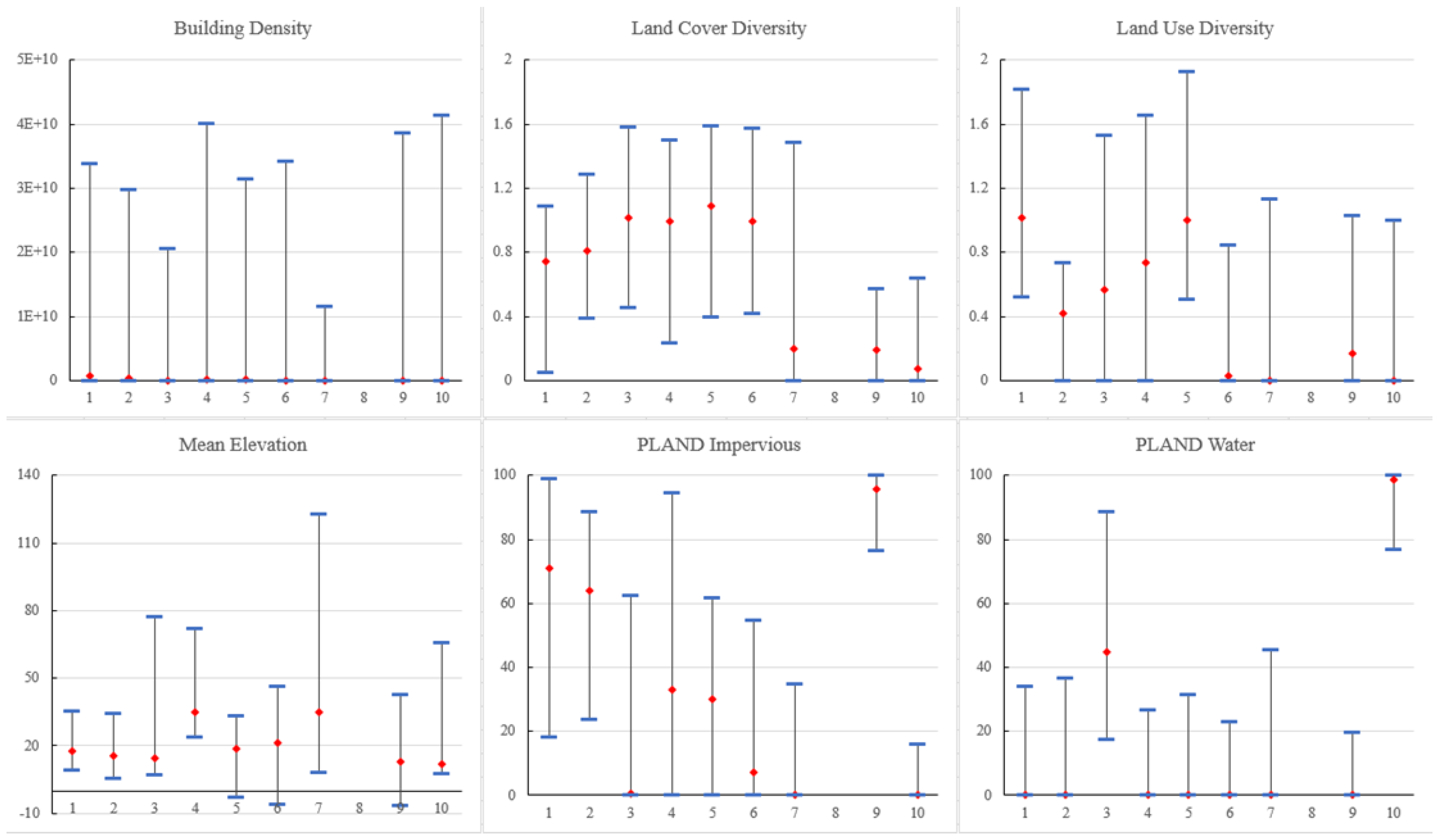
Based on the quantitative measure of clustering performance (i.e., AIC), visual inspection of the produced landscape types and our contextual knowledge of the study area, we selected the 10th solution of model no. 7. Table 3 shows the proportional distribution of clusters. As seen, Cluster 6 takes up 18.7% of Singapore’s total land area making it the largest cluster, and Cluster 8 occupying 0.6% is the smallest cluster among all. Fig. 2 shows the spatial distribution of the ten landscape types across Singapore and an illustrative sample to represent each landscape type. How the landscape types compare with regard to each of the 6 variables used in creating the model for clustering can be seen in Fig. 3. The two major land uses composing each of the landscape types are also provided in Table 3 for comparison. We decided to ignore Cluster 8 during the further analyses since Cluster 8 only occupied 0.6% of Singapore's land, making it challenging to draw enough random samples, and also because Cluster 8 had an unexpectedly high BD in comparison with other clusters. Including it would have resulted in masking of the variations in BD among clusters, negatively affecting the translation of the clusters into categories (Table 2) to be used in accuracy assessment. The landscape types (Table 2) are arranged by their respective ordinal category (i.e., from very high to very low) in relation to the variables ordered based on their relative importance as identified by running a Decision Tree (DT) classifier employing the CRT method of growing—the variables based on their respective relative importance were: PLAND IS, LC Diversity, LU Diversity, ME, PLAND W, and BD. In the event that multiple landscape types were in the same ordinal category in relation to a given variable, their category in the next important variable was taken as a reference to order them. For instance, landscape types no. 1 and 2 were the same regarding both PLAND IS and LC Diversity, but UTL no. 1 was ordered higher than landscape type no. 2 since landscape type no. 1 had high LU Diversity, while landscape type no. 2 had medium LU Diversity. Table 1. The percent area of Singapore occupied by each ULT, and the two major land uses composing each of the ULTs.
| ULT Number | Proportional Size of ULT (%) | Major Two Constituent Land Uses |
| 1 | 16.7 | Residential (51.5%) and Commercial-Industrial (23.5%) |
| 2 | 11.8 | Commercial-Industrial (34.5) and Residential (31.9%) |
| 3 | 4.9 | Water Bodies (39.2%) and Open Space (28%) |
| 4 | 7.6 | Residential (41.5%) and Open Space (11.2%) |
| 5 | 16.4 | Residential (33.9%) and Road (13.6%) |
| 6 | 18.7 | Transport-Special Use (21.5%) and Open Space (17.8%) |
| 7 | 10.2 | Open Space (67.2%) and Reserve (11.1%) |
| 8 | 0.6 | Transport-Special Use (38.9%) and Commercial-Industrial (26.4%) |
| 9 | 10.7 | Commercial-Industrial (57.7%) and Transport-Special Use (19.6%) |
| 10 | 2.2 | Water Bodies (92.5%) and Open Space (2.75%) |
Figure 2.
Spatial distribution of each of the ten ULT’s across Singapore, in addition to one sample to illustrate each ULT.
Figure 2.
Spatial distribution of each of the ten ULT’s across Singapore, in addition to one sample to illustrate each ULT.
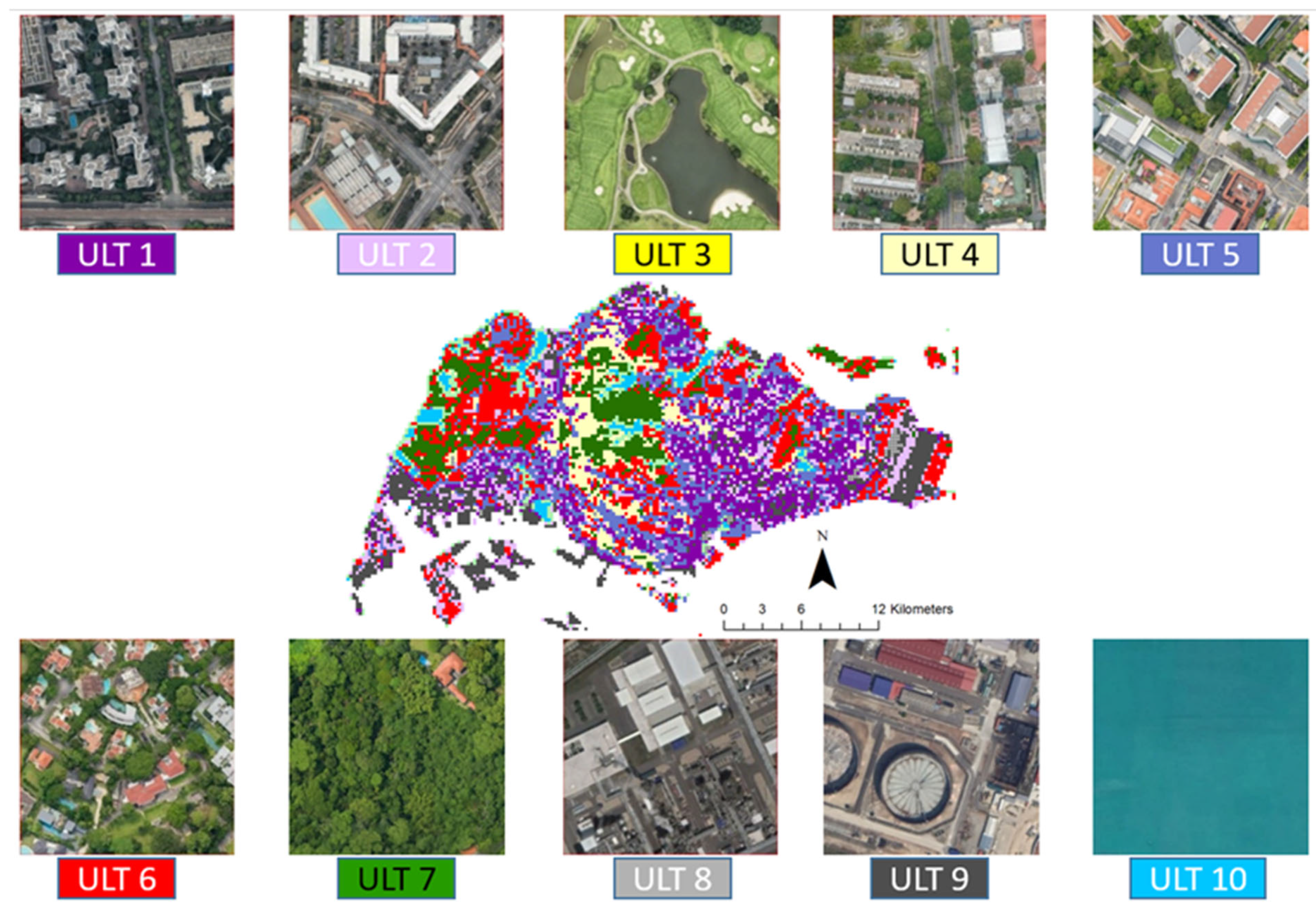
Figure 3.
Minimum, maximum and median value of each of the six variables used in the final clustering model across ULT’s. ULT no. 8 was removed from analysis.
Figure 3.
Minimum, maximum and median value of each of the six variables used in the final clustering model across ULT’s. ULT no. 8 was removed from analysis.
3.2. Environmental Relevance of the Produced ULT
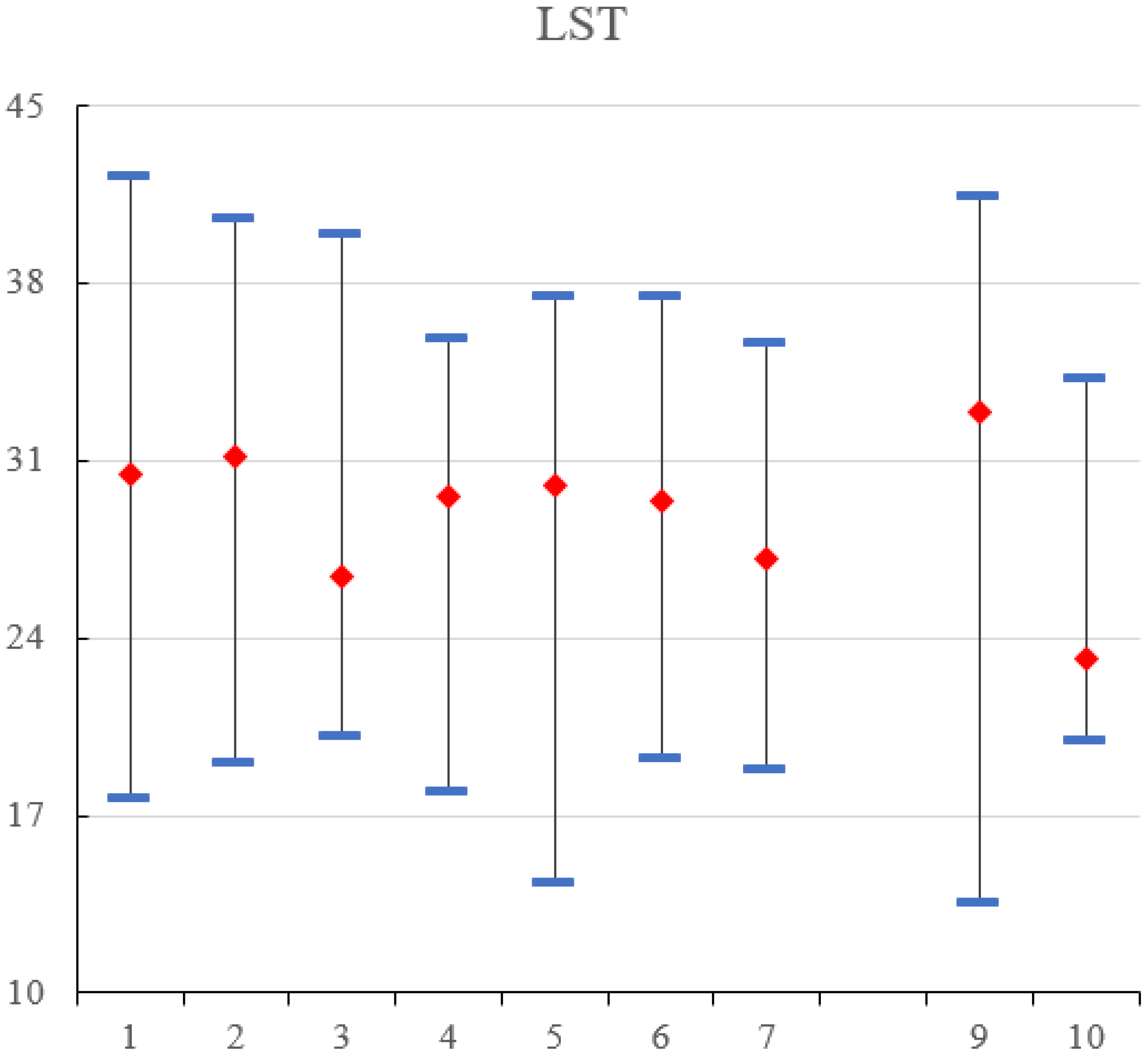
ANOVA results demonstrated that the produced landscape types had statistically significant different LSTs (F Statistic: 487.5, p < 0.01; Welch Statistic: 509.9, p < 0.01). According to the post-hoc tests (not shown for brevity), all the landscape types pairs had distinct LSTs. As Fig. 4 illustrates, landscape type no. 9 was associated with the highest median LST and landscape type no. 10 had the lowest median LST among all.
Figure 4.
Minimum, maximum, and median value of LST across ULT’s. ULT no. 8 was removed from analysis.
Figure 4.
Minimum, maximum, and median value of LST across ULT’s. ULT no. 8 was removed from analysis.
3.3. Practical Relevance of the Produced ULT
As mentioned earlier, we used our interactive pilot session to identify how we could improve the way in which we conducted our accuracy assessment exercise by requesting feedback from the participants. We made multiple changes as a result. For instance, the aim of the exercise was elaborated during the presentation preceding the exercise to provide the participants with the context within which the study was being conducted. Also, we put on both the presentation slides and the sheets circulated among the participants three illustrative samples next to each of the landscape type and described them in relation to the variables characterising landscape types were produced. This was done to provide the participants with a clear mind upfront regarding what was being asked of them to complete.

Table 4.
and 5 describe the outcome of the two separate sessions—with students and practitioners of urban planning and design—that were conducted. The overall accuracies were 71.6% and 60%, respectively. Based on the confusion matrices (Table 4), the major sources of confusion during the first session were between landscape type no. 2 and 9, and 4 and 5, and in the second session were between 4 and 5, and 3 and 7. Table 2. Confusion matrix describing the outcome of the validation exercise conducted with students of urban design at NUS.
| ULT | 1 | 2 | 3 | 4 | 5 | 6 | 7 | 9 | 10 | Total |
|---|---|---|---|---|---|---|---|---|---|---|
| 1 | 14 | 3 | 1 | 77.8% | ||||||
| 2 | 2 | 10 | 1 | 5 | 55.6% | |||||
| 3 | 15 | 1 | 2 | 83.3% | ||||||
| 4 | 1 | 14 | 3 | 77.8% | ||||||
| 5 | 3 | 10 | 2 | 3 | 55.6% | |||||
| 6 | 1 | 1 | 1 | 13 | 2 | 72.2% | ||||
| 7 | 2 | 2 | 13 | 1 | 72.2% | |||||
| 9 | 1 | 5 | 2 | 10 | 55.6% | |||||
| 10 | 1 | 17 | 94.4% | |||||||
| Total | 18 | 18 | 18 | 18 | 18 | 18 | 18 | 18 | 18 | 71.6% |
Table 5.
Confusion matrix describing the outcome of the validation exercise conducted with urban practitioners at SCP Consultants Private Limited.
Table 5.
Confusion matrix describing the outcome of the validation exercise conducted with urban practitioners at SCP Consultants Private Limited.
| ULT | 1 | 2 | 3 | 4 | 5 | 6 | 7 | 9 | 10 | Total |
|---|---|---|---|---|---|---|---|---|---|---|
| 1 | 10 | 1 | 90.1% | |||||||
| 2 | 1 | 5 | 2 | 2 | 1 | 45.5% | ||||
| 3 | 5 | 1 | 5 | 45.5% | ||||||
| 4 | 2 | 3 | 5 | 1 | 27.3% | |||||
| 5 | 3 | 4 | 3 | 1 | 27.3% | |||||
| 6 | 2 | 9 | 81.8% | |||||||
| 7 | 4 | 1 | 6 | 54.5% | ||||||
| 9 | 1 | 2 | 1 | 7 | 63.6% | |||||
| 10 | 11 | 100% | ||||||||
| Total | 11 | 11 | 11 | 11 | 11 | 11 | 11 | 11 | 11 | 59.6% |
4. Discussion
Urban ecology has progressed significantly as a discipline, knowledge has been generated in multiple areas that can help in making more informed decisions regarding the afore-mentioned issues, but there seems to be a gap between knowledge generation and its application (McDonnell & Hahs, 2013). In other words, the efficient and effective transfer of urban ecological knowledge into practice is required to build cities that are sustainable, liveable, healthy and resilient (McDonnell & MacGregor-Fors, 2016). In order to facilitate the efficient and effective transfer of this knowledge, bridging the gap between the urban scientific knowledge base and the practice of designing and building cities is required (McDonnell, 2015). Two of the major impediments to this information transfer are discussed below.
First, there is a communication barrier, as terminology and media used by urban ecologists is commonly not readily accessible to urban practitioners. While scientists report their findings in the form of mathematical and statistical models, urban planners and designers express and communicate their thoughts primarily using visual mediums. Second, scientific research usually studies the effect of individual variables by isolating the effects of other variables. For instance, the effect of vegetation on air pollution is examined by ensuring that other variables with potential impact on air pollution (e.g., the level of background pollution, distance to the polluting sources, surrounding land use) remain constant to ensure the observed impact is solely due to the differences in the vegetation structure. Conversely, an urban design or planning proposal encompasses a combination of different landscape elements as 2D and increasingly 3D models in which knowledge on the interaction among numerous urban variables is required. Therefore, urban practitioners may not find scientific papers readily understandable or effective in communicating key concepts. Landscape typologies therefore hold potential as a boundary object that can facilitate bridging the gap between science and practice.
4.1. ULT for a Compact City
In this study we produced a ULT—consisting of ten landscape types—for the compact city of Singapore. We built our ULT upon an extended version of the conceptual framework suggested by Wentz et al. (2018) that incorporates aspects of land cover, configuration, elevation, and land use. This ULT is thus built upon a broader conceptual framework than previous similar studies (Cadenasso et al., 2007; Hamstead et al., 2016; Larondelle, Hamstead, Kremer, Haase, & McPhearson, 2014; Stewart & Oke, 2012). We chose to include these variables as their importance in relation to environmental and ecological processes has been established by past research. For instance, XXX (masked for blind review) demonstrated that different land uses in XXX had distinct temperature signatures for their effect on the spatial pattern of vegetation. A similar observation was made in the City of Indianapolis, USA (Wilson et al., 2003). The configuration of vegetation patches has also been shown to affect air (Liu & Shen, 2014) and water (Ouyang et al., 2010) pollution, LST (Masoudi et al., 2019), and biodiversity (Prevedello et al., 2017).
The afore-mentioned variables of land use, elevation and configuration had substantial impacts in influencing the resulting landscape types in our study. For instance, landscape type no. 4 and 5 in our study were only different in their elevation, and LC Diversity was the variable that caused ULTs no. 6 and 7 to be identified as distinct landscape types. landscape types no. 1 and 2 also seem to have been differentiated mainly based on LU Diversity. These landscape types would not have been differentiated from each other according to conceptual frameworks that do not consider these novel aspects of urban form, such as the LCZ (Stewart & Oke, 2012), HERCULES (Cadenasso et al., 2007) or STURLA (Hamstead et al., 2016). In fact, the two variables of land use and land cover diversity emerged as second and third most important variables in determining the clusters, which demonstrates the importance of these variables to the spatial pattern of urban landscapes. Conversely, building density/height is a main determinant in landscape types, such as LCZ (Stewart & Oke, 2012) and STURLA (Hamstead et al., 2016) and that was shown in our study to have the least relative importance by the DT classifier. This may be because in a compact city like Singapore that is filled with high-rise buildings, the building density variable is not going to drive much of a variation, causing this variable to not play a major role in determining landscape types. This is in contrast to studies in European or North American cities that may be more sprawling and thus have variation in building height depending on the distance from the central zone. This finding reiterates that the choice of variables is dependent upon the specific research questions and objectives, as well as characteristics of the city, encouraging urban ecological studies to use more explicit question-driven variables (McDonnell & Hahs, 2013).
4.2. The Produced ULT Can Predict Thermal Outcomes
Few previous studies have tested their ULTs against LST to analyze the effectiveness of the ULTs in predicting environmental performance (Bechtel et al., 2019; Hamstead et al., 2016; Larondelle, Hamstead, Kremer, Haase, & McPherson, 2014; Stewart et al., 2014). Our ANOVA and post-hoc tests results revealed that all possible pairs of landscape types in our ULT had statistically significant different LSTs. In other words, the landscape types we produced had distinct temperature signatures. According to our findings, a landscape type that has a high level of impervious surface, low levels of land cover and land use diversity, is dense and located on a lower elevation is expected to be warmer than a landscape type with opposite pattern. For example, landscape type no. 9 is mainly (75%) consisted of commercial-industrial and transportation-special use land uses and expectedly has a very high PLAND IS, very low LC Diversity, low LU Diversity, very low PLAND W and low BD. Expectedly, this landscape type was associated with the highest LST among all. Spatially, landscape type no. 9 can largely be found in the east and south-west of Singapore, where the airport and major industrial sites are located (Fig. 2). landscape type no. 2 and 1 followed landscape type no. 9 in LST. These two landscape types were observed to have high PLAND IS and medium LC Diversity, with high and medium BD, respectively, which could perhaps explain the high LST for these landscape types. Residential and commercial-industrial were the two major land uses composing these landscape types—in reverse order though—and both of these land uses were previously shown to have relatively higher LSTs compared to other land uses in XXX (masked for blind review). In fact, the commercial-industrial land use has previously been shown to have the highest LST among studied land uses (XXX, masked for blind review). Visual inspection demonstrates that landscape type no. 1 is comprised mainly of high-rise residential buildings that could explain its relatively higher BD in comparison with landscape type no. 2. One would probably expect landscape type no. 1 to be warmer than landscape type no. 2 since the two landscape types have same level of PLAND IS and LC Diversity; however, landscape type no. 1 had higher level of BD, and denser neighbourhoods are generally understood to be warmer (Wilson et al., 2003). However, it should be highlighted that landscape type no. 1 is located on a relatively higher elevation than landscape type no. 2, which would have probably driven its LST lower than that for landscape type no. 2. Similar observation about the importance of elevation was observed for landscape type no. 4 and 5. Not only did the elevation variable result in distinction of these two landscape types—as also mentioned earlier—but these two landscape types were also observed to have distinct LSTs, with landscape type no. 5 being warmer as it has generally lower elevation than landscape type no. 4. These observations further underscore the importance of elevation that is entirely overlooked in existing landscape type.
The remaining landscape types that had relatively lower LSTs had very low PLAND IS and BD, with open space, water bodies, and reserve as their major constituent land uses. This finding is also in line with what was observed in a previous study in XXX that found open space to have the lowest LST and reserve land use as the fourth land use with low LST (XXX, masked for blind review). Water bodies were also observed to be consistently cooler than other land covers (Masoudi & Tan, 2019). Studies elsewhere also observed that landscape types with a higher proportion of vegetation or water were generally associated with lower LST (Hamstead et al., 2016; Larondelle, Hamstead, Kremer, Haase, & McPherson, 2014). Landscape type no. 10 and 3 had the lowest LSTs among all since both had very high PALND W. Ninety-two percent of landscape type no. 10 consisted of water bodies. Water bodies and open space land uses also comprised 39.2% and 28% of landscape type no. 3, respectively. Between landscape types no. 6 and 7, landscape type no. 7 was observed to have a lower LST, which could be explained by a combination of higher proportion of open space land use, higher elevation and higher LC Diversity. Given the very low PLAND IS, higher LC Diversity for landscape type no. 7 would mean a greater mixture of vegetation and water land covers both of which would have contributed to the observed lower LST for landscape type no. 7. Landscape type no. 7 mainly exists in the Central and Western Catchment areas and the Pulau Ubin island in the north-east of the main island.
4.3. Urban Planners and Designers Are Able to Use the Produced ULT
As far as we could ascertain, no previous study has attempted to see if landscape types could be used by urban planners and designers, limiting the probability of the produced science being incorporated into practice. We showed in our study that the landscape types we produced were generally recognizable by landscape architect, design and planning students and practicing urban planners and designers. Putting this finding next to our results on the environmental relevance of the produced ULT, we feel that our ULT could enable urban planners and designers to evaluate the environmental performance of their alternative urban development scenarios. This would provide a means by which urban ecological knowledge can be transferred into practice, a requirement towards achieving urban sustainability (McDonnell & Hahs, 2013). Among the landscape types, landscape types no. 4 and 5 were the major source of error as they were mistaken for one another in both sessions of the validation exercise. It should be highlighted that these two landscape types were only different in terms of elevation, which could be challenging to differentiate based on 2D pictures. Despite this fact, we decided to keep them both as we assumed elevation would play an important role in determining landscape types and influencing key environmental and ecological processes as also later supported by our findings.
4.4. Methodological Novelties and Future Research Directions
The importance of considering the complex interactions among different components and processes in creating the structure of urban ecosystems has been pointed out by previous studies (Alberti, 2005; Hamstead et al., 2016; Larondelle, Hamstead, Kremer, Haase, & McPherson, 2014). These studies have raised the important point that individual components should not be studied in isolation if we are to unravel how the urban ecosystem as highly complex social-ecological-technological system works. However, we argue that the methodology employed by previous studies, which relied on pre-defining the combination of variables, may not be able to adequately capture the interactions among variables (Hamstead et al., 2016; Larondelle, Hamstead, Kremer, Haase, & McPhearson, 2014). We believe that the methodology that we introduced in this paper is capable of accounting for the interactions among variables by avoiding defining possible landscape types a priori, and allowing the emergent structures to form based on dynamic interactions among variables. A similar approach was previously taken by Van Eetvelde & Antrop (2009); however, the scale of their study was the whole country of Belgium, while our study examined the suitability of the approach at the city-scale, with a compact form of urban development.
As mentioned earlier in Section 3.1., we added PLAND W to the variables of model no. 6 following the visual inspection of the produced landscape types. Adding PLAND W could produce more meaningful landscape types because of the specific distributional pattern of water bodies in Singapore. Water in Singapore is not as mixed with vegetation and impervious surface land covers as these two land covers are mixed with each other. This has resulted in water patches being concentrated in a small area, with the majority of analytical units lacking water content. Therefore, not including a metric to consider water would have caused the error of clustering to increase.
Overall, we believe that the ULT developed by our research project could help advance the existing knowledge on quantifying urban structure and its relationship to ecological and environmental processes, as well as facilitate transferring the urban ecological knowledge into practice. It should, however, be emphasized that since aspects of urban structure do interact with one another and follow a feedback mechanism, the relative importance of different variables may vary over time and space depending on the current structure as also demonstrated by previous studies (Masoudi et al., 2019, 2021). In view of this, we argue that while it may not be possible to develop a universal ULT, our overall methodology and general qualitative description of landscape types should be transferrable to other cities. We also believe that with studies applied to cities of different climates, socio-economic settings and spatial structures, commonalities would be observable (Hahs et al., 2009). It is also recommended that future research consider testing their ULT against other variables of environmental and ecological performance than only temperature to enhance the usefulness of the ULT for urban planners and designers.
5. Conclusions
We believe that ULT can be an effective approach to condensing complex urban ecological knowledge that fits into current planning and design practices since ULT can overcome the language barrier that exists between science and practice and communicate knowledge in the same format (e.g., 2D and 3D maps) as being used by urban practitioners. Therefore, utilizing a novel computational approach, we developed a ULT for the compact city of Singapore based on a conceptual framework informed by recent advances in urban ecology, with the aim of identifying ULT that is distinguishable by urban practitioners and able to predict environmental performance indicators. Our conceptual framework included 15 variables from five main components of urban form, namely land cover composition and configuration, land use, building density, and elevation.
Our results showed that students and professionals of urban planning and design were able to sufficiently distinguish different landscape types, returning overall scores of 71.6% and 60% on the confusion matrices, respectively. Additionally, examining our ULT against LST as an importance indicator of environmental performance demonstrated the environmental relevancy of the ULT that we produced, where the LST signature of each landscape type was found to be significantly different from all others. Our findings indicate that our ULT can effectively be employed as a tool by urban practitioners and help them make more informed decisions regarding the environmental outcomes of various urban development proposals towards building cities that are sustainable, healthy, liveable and resilient.
While our ULT was produced based on Singapore-specific dataset, we believe that our overall methodological approach is replicable across cities of different characteristics. Furthermore, it is likely that our ULT would be applicable to other compact cities with some adjustments. Future studies can examine such a possibility and also investigate if the additional variables (i.e., land use, spatial configuration and elevation) that were found useful in our study will be effective in identifying more powerful ULTs in other cities. We encourage future studies to examine ULTs against other environmental and social indicators. More evidence on the predictive ability of ULTs can help increase their take-up rate by urban practitioners and facilitate knowledge mobilization.
Supplementary Material
The following supporting information can be downloaded at the website of this paper posted on Preprints.org.
References
- Alberti, M. (2005). The Effects of Urban Patterns on Ecosystem Function. International Regional Science Review, 28(2), 168–192. [CrossRef]
- Alberti, M. (2007). Ecological Signatures: The Science of Sustainable Urban Forms. Places, 19(3), 56–60.
- Anderson, J. R., Hardy, E. E., Roach, J. T., & Witmer, R. E. (1976). A land use and land cover classification system for use with remote sensor data.
- Bechtel, B., Demuzere, M., Mills, G., Zhan, W., Sismanidis, P., Small, C., & Voogt, J. (2019). SUHI analysis using Local Climate Zones—A comparison of 50 cities. Urban Climate, 28(January), 100451. [CrossRef]
- Cadenasso, M. L., Pickett, S. T., & Schwarz, K. (2007). Spatial heterogeneity in urban ecosystems: Reconceptualizing land cover and a framework for classification. Frontiers in Ecology and the Environment, 5(2), 80–88. [CrossRef]
- Congalton, R. G., & Green, K. (2019). Assessing the Accuracy of Remotely Sensed Data: Principles and Practices (Third). CRC Press Inc.
- Connors, J. P., Galletti, C. S., & Chow, W. T. L. (2013). Landscape configuration and urban heat island effects: Assessing the relationship between landscape characteristics and land surface temperature in Phoenix, Arizona. Landscape Ecology, 28(2), 271–283. [CrossRef]
- Department of Statistics Singapore. (2020). Population Trends 2020.
- Dissegna, M. A., Yin, T., Wei, S., Richards, D., & Grêt-Regamey, A. (2019). 3-D reconstruction of an urban landscape to assess the influence of vegetation in the radiative budget. Forests, 10(8), 1–19. [CrossRef]
- Forman, R. T. T. (2014). Urban Ecology: Science of Cities. Cambridge University Press. [CrossRef]
- Forman, R. T. T., & Godron, M. (1986). Landscape Ecology. Jhon Wiley & Sons.
- Frye, C. (n.d.). About the Geometrical Interval classification method. Retrieved September 1, 2018, from https://www.esri.com/arcgis-blog/products/product/mapping/about-the-geometrical-interval-classification-method/.
- George, D., & Mallery, P. (2019). IBM SPSS Statistics 26 Step by Step A Simple Guide and Reference. Routledge.
- Government Technology Agency. (n.d.). Master Plan 2014 Land Use. Retrieved August 1, 2018, from https://data.gov.sg/dataset/master-plan-2014-land-use?resource_id=0d1a6cda-7cad-4b17-b9a8-9e173afebbc1.
- Hahs, A. K., & McDonnell, M. J. (2006). Selecting independent measures to quantify Melbourne’s urban-rural gradient. Landscape and Urban Planning, 78(4), 435–448. [CrossRef]
- Hahs, A. K., McDonnell, M. J., & Breuste, J. H. (2009). A comparative ecology of cities and towns: Synthesis of opportunities and limitations. In A. K. Hahs, M. J. McDonnell, & J. H. Breuste (Eds.), Ecology of Cities and Towns: A Comparative Approach (pp. 574–596). Cambridge University Press. [CrossRef]
- Hamstead, Z. A., Kremer, P., Larondelle, N., McPhearson, T., & Haase, D. (2016). Classification of the heterogeneous structure of urban landscapes (STURLA) as an indicator of landscape function applied to surface temperature in New York City. Ecological Indicators, 70, 574–585. [CrossRef]
- Hochberg, Y., & Tamhane, A. C. (1987). Multiple Comparison Procedures (Y. Hochberg & A. C. Tamhane, Eds.). John Wiley & Sons, Inc. [CrossRef]
- Larondelle, N., Hamstead, Z. A., Kremer, P., Haase, D., & McPhearson, T. (2014). Applying a novel urban structure classification to compare the relationships of urban structure and surface temperature in Berlin and New York City. Applied Geography, 53, 427–437. [CrossRef]
- Larondelle, N., Hamstead, Z. A., Kremer, P., Haase, D., & McPherson, T. (2014). Applying a novel urban structure classification to compare the relationships of urban structure and surface temperature in Berlin and New York City. Applied Geography, 53, 427–437. [CrossRef]
- Liu, H. L., & Shen, Y. S. (2014). The impact of green space changes on air pollution and microclimates: A case study of the taipei metropolitan area. Sustainability (Switzerland), 6(12), 8827–8855. [CrossRef]
- Masoudi, M., & Tan, P. Y. (2019). Multi-year comparison of the effects of spatial pattern of urban green spaces on urban land surface temperature. Landscape and Urban Planning, 184. [CrossRef]
- Masoudi, M., Tan, P. Y., & Fadaei, M. (2021). The effects of land use on spatial pattern of urban green spaces and their cooling ability. Urban Climate, 35(November 2020), 100743. [CrossRef]
- Masoudi, M., Tan, P. Y., & Liew, S. C. (2019). Multi-city comparison of the relationships between spatial pattern and cooling effect of urban green spaces in four major Asian cities. Ecological Indicators, 98(November 2018), 200–213. [CrossRef]
- McDonnell, M. J. (2015). Journal of Urban Ecology: Linking and promoting research and practice in the evolving discipline of urban ecology. Journal of Urban Ecology, 1(1), juv003. [CrossRef]
- McDonnell, M. J., & Hahs, A. K. (2013). The future of urban biodiversity research: Moving beyond the “low-hanging fruit.” Urban Ecosystems, 16(3), 397–409. [CrossRef]
- McDonnell, M. J., & MacGregor-Fors, I. (2016). The ecological future of cities. Science, 352(6288), 936–938. [CrossRef]
- McGarigal, K., Cushman, S. A., & Ene, E. (2012). FRAGSTATS v4: Spatial Pattern Analysis Program for Categorical and Continuous Maps. Computer Software Program Produced by the Authors at the University of Massachusetts, Amherst.
- McGarigal, K., & Marks, B. J. (1995). Spatial pattern analysis program for quantifying landscape structure. Gen. Tech. Rep. PNW-GTR-351.
- Messerli, P., Heinimann, A., & Epprecht, M. (2009). Finding homogeneity in heterogeneity—A new approach to quantifying landscape mosaics developed for the Lao PDR. Human Ecology, 37(3), 291–304. [CrossRef]
- Mücher, C. A., Klijn, J. A., Wascher, D. M., & Schaminée, J. H. J. (2010). A new European Landscape Classification (LANMAP): A transparent, flexible and user-oriented methodology to distinguish landscapes. Ecological Indicators, 10(1), 87–103. [CrossRef]
- Ouyang, W., Skidmore, A. K., Toxopeus, A. G., & Hao, F. (2010). Long-term vegetation landscape pattern with non-point source nutrient pollution in upper stream of Yellow River basin. Journal of Hydrology, 389(3–4), 373–380. [CrossRef]
- Pataki, D. E., Alberti, M., Cadenasso, M. L., Felson, A. J., McDonnell, M. J., Pincetl, S., Pouyat, R. V., Setälä, H., & Whitlow, T. H. (2021). The Benefits and Limits of Urban Tree Planting for Environmental and Human Health. Frontiers in Ecology and Evolution, 9(April), 1–9. [CrossRef]
- Prevedello, J. A., Almeida-Gomes, M., & Lindenmayer, D. B. (2017). The importance of scattered trees for biodiversity conservation: A global meta-analysis. Journal of Applied Ecology, 0–3. [CrossRef]
- Richards, D., Fung, T., Belcher, R., & Edwards, P. (2020). Differential air temperature cooling performance of urban vegetation types in the tropics. Urban Forestry & Urban Greening, 50(March), 126651. [CrossRef]
- Ridd, M. K. (1995). Exploring a V-I-S (vegetation-impervious surface-soil) model for urban ecosystem analysis through remote sensing: Comparative anatomy for cities. International Journal of Remote Sensing, 16(12), 2165–2185. [CrossRef]
- Simensen, T., Halvorsen, R., & Erikstad, L. (2018). Methods for landscape characterisation and mapping: A systematic review. Land Use Policy, 75(April), 557–569. [CrossRef]
- Singapore Department of Statistics. (2022). Households. https://www.singstat.gov.sg/find-data/search-by-theme/households/households/latest-data.
- Stewart, I. D., & Oke, T. R. (2012). Local climate zones for urban temperature studies. Bulletin of the American Meteorological Society, 93(12), 1879–1900. [CrossRef]
- Stewart, I. D., Oke, T. R., & Krayenhoff, E. S. (2014). Evaluation of the “local climate zone” scheme using temperature observations and model simulations. International Journal of Climatology, 34(4), 1062–1080. [CrossRef]
- Tan, P. Y., & Abdul Hamid, A. R. bin. (2014). Urban ecological research in Singapore and its relevance to the advancement of urban ecology and sustainability. Landscape and Urban Planning, 125, 271–289. [CrossRef]
- Tan, P. Y., Liao, K.-H., Hwang, Y. H., & Chua, V. (2018). Nature, Place & People: Forging Connections through Neighbourhood Landscape Design. WORLD SCIENTIFIC. [CrossRef]
- Tratalos, J., Fuller, R. A., Warren, P. H., Davies, R. G., & Gaston, K. J. (2007). Urban form, biodiversity potential and ecosystem services. Landscape and Urban Planning, 83(4), 308–317. [CrossRef]
- Turner, M. G. (1989). Landscape Ecology: The Effect of Pattern on Process. Annual Review of Ecology and Systematics, 20(1), 171–197. [CrossRef]
- Van Eetvelde, V., & Antrop, M. (2009). A stepwise multi-scaled landscape typology and characterisation for trans-regional integration, applied on the federal state of Belgium. Landscape and Urban Planning, 91(3), 160–170. [CrossRef]
- Wang, H., & Tassinary, L. G. (2019). Effects of greenspace morphology on mortality at the neighbourhood level: A cross-sectional ecological study. The Lancet Planetary Health, 3(11), e460–e468. [CrossRef]
- Wentz, E. A., York, A. M., Alberti, M., Conrow, L., Fischer, H., Inostroza, L., Jantz, C., Pickett, S. T. A., Seto, K. C., & Taubenböck, H. (2018). Six fundamental aspects for conceptualizing multidimensional urban form: A spatial mapping perspective. Landscape and Urban Planning, 179(July), 55–62. [CrossRef]
- Wilson, J. S., Clay, M., Martin, E., Stuckey, D., & Vedder-Risch, K. (2003). Evaluating environmental influences of zoning in urban ecosystems with remote sensing. Remote Sensing of Environment, 86(3), 303–321. [CrossRef]
Figure 1.
The conceptual framework used to collect data on spatial structure of urban landscape. The framework is adopted from Wentz et al. (2018).
Figure 1.
The conceptual framework used to collect data on spatial structure of urban landscape. The framework is adopted from Wentz et al. (2018).
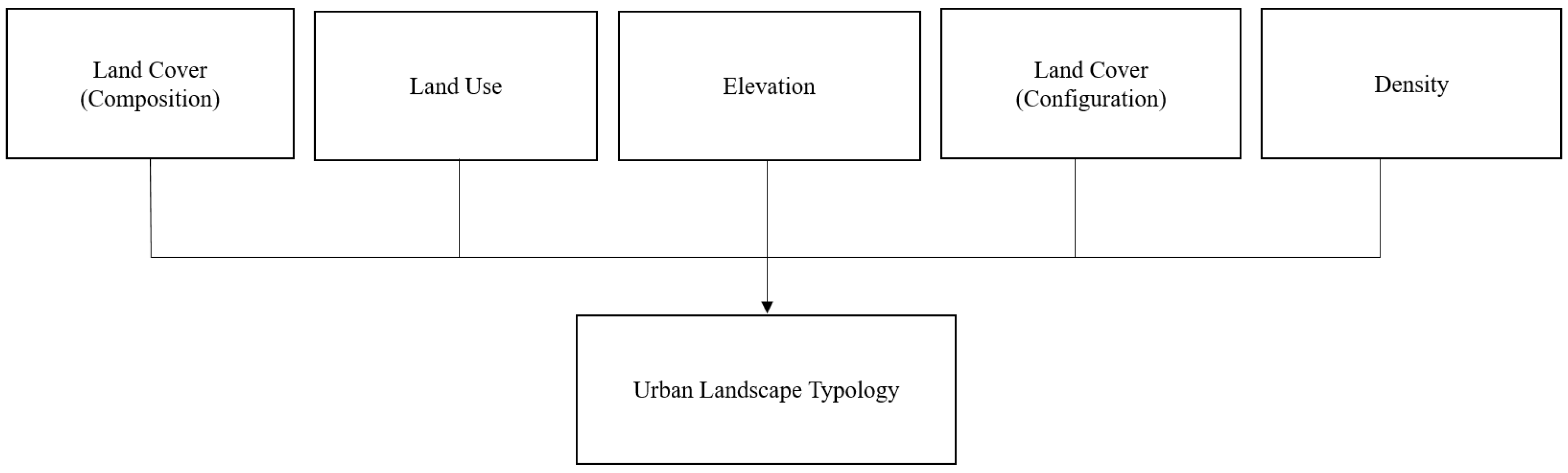
Table 1.
Landscape metrics employed to characterize the spatial pattern of land cover and land use in this research. You may refer to (McGarigal & Marks, 1995) for more details on the metrics.
Table 1.
Landscape metrics employed to characterize the spatial pattern of land cover and land use in this research. You may refer to (McGarigal & Marks, 1995) for more details on the metrics.
| Landscape Metric | Abbreviation | Description | Unit |
|---|---|---|---|
| Percentage of Landscape | PLAND | The proportional area occupied by a given patch type | Percent |
| Patch Density | PD | The number of patches of a given type over landscape’s total area | Number per 100 hectares |
| Shannon’s Diversity Index | SHDI | A composite measure of patch richness and proportional area of different patch types | Information |
Table 2.
Qualitative description of ULTs. The order of the ULTs is based on the ordinal category of variables ordered based on their relative importance as identified by the decision tree classifier.
Table 2.
Qualitative description of ULTs. The order of the ULTs is based on the ordinal category of variables ordered based on their relative importance as identified by the decision tree classifier.
| ULT Number | ULT Components | |||||
|---|---|---|---|---|---|---|
| PLAND IS | LC DIVERSITY | LU DIVERSITY | ME | PLAND W | BD | |
| 9 | Very high | Very low | Low | Low | Very low | Low |
| 1 | High | Medium | High | Medium | Very low | High |
| 2 | High | Medium | Medium | Low | Very low | Medium |
| 4 | Medium | High | High | High | Very low | Medium |
| 5 | Medium | High | High | Medium | Very low | Medium |
| 3 | Very low | High | Medium | Low | Very high | Very low |
| 6 | Very low | High | Very low | Medium | Very low | Very low |
| 7 | Very low | Very low | Very low | High | Very low | Very low |
| 10 | Very low | Very low | Very low | Low | Very high | Very low |
Disclaimer/Publisher’s Note: The statements, opinions and data contained in all publications are solely those of the individual author(s) and contributor(s) and not of MDPI and/or the editor(s). MDPI and/or the editor(s) disclaim responsibility for any injury to people or property resulting from any ideas, methods, instructions or products referred to in the content. |
© 2024 by the authors. Licensee MDPI, Basel, Switzerland. This article is an open access article distributed under the terms and conditions of the Creative Commons Attribution (CC BY) license (http://creativecommons.org/licenses/by/4.0/).
Copyright: This open access article is published under a Creative Commons CC BY 4.0 license, which permit the free download, distribution, and reuse, provided that the author and preprint are cited in any reuse.


