Forecasting and Intervention Time Series Analysis Using Autoregressive Integrated Moving Average (ARIMA) Models: Evaluating the impact of 2018 and 2021 Rift Valley Fever Outbreaks on Kenyan food Price Index

1. Introduction

In recent years, there has been an increase in the number of infectious disease outbreaks in sub-Saharan Africa, which poses a threat to the food security [1]. Food security pillars; availability, access, utilization, and stability are central to economic sustainability, especially in regions susceptible to agricultural shocks [2]. Many countries in Africa are not able to effectively control these infectious disease outbreaks due to their limited capacity to predict and manage the risks using the most appropriate intervention measures, and Kenya is not an exception in this case [3]. Kenya, a country with diverse climatic regions and varying access to markets, faces food price volatility influenced by environmental factors, market dynamics, and external shocks like infectious disease outbreaks [4]. The first outbreak of RVF was first reported in Kenya in 1930 [5] , and since then, there have been several outbreaks, the most recent of which occurred in 2015/2016, 2018 and 2021. Being a zoonotic disease, RVF outbreaks are significant events to food security. RVF impacts livestock health, restricts market access, and drives up food prices, affecting food security and household economic stability [6].

Multiple RVF outbreaks have occurred in Kenya, where the agricultural sector contributes largely to the economy's growth [7]. These outbreaks have adverse effects on the food prices of commonly consumed items, especially animal-based foods [8]. Proper and timely interpretations of the food price dynamics are crucial for the key policymakers and stakeholders who work towards taking mitigation measures to control such shocks in the economy [9]. Several studies have used ARIMA and intervention time series methodologies to forecast food prices and disease outbreaks both in Kenya and beyond. For instance, [11] used the intervention time series approach to investigate the impact of Free Maternal Health Care on the child’s infant mortality. During the COVID-19 era, [12] did a study on the interruption time series analysis of the impact of COVID-19 on the epidemic trend of gonorrhea in China using ARIMA model. [13] Used an Artificial-Intelligence-Based Time-Series Intervention Model to assess the impact of the COVID-19 pandemic on tomato supply and prices in Hyderabad, India.

This study uses an ARIMA time series modeling approach to analyze food price trends across various Kenyan towns and assess the impact of the RVF outbreak on market prices. Time series data, including historical price indices, were collected for the major towns in Kenya. Following data validation and stationarity testing, ARIMA models were developed for each town's food price index to understand both baseline price trends and the influence of RVF on price fluctuations. Intervention analysis was applied to evaluate the extent of the outbreak's impact on food prices, providing insights into both the immediate and longer-term effects on food markets.

This research aimed at using the commonly used ARIMA model to forecast a two-year food price index with close consideration to the most recent RVF outbreaks in Kenya. To quantify and analyze the effect of RVF outbreaks on food prices, the study further employed the intervention time series model to measure the impact of the 2018 and 2021 RVF outbreaks [10]. The integration of the two time series approaches was expected to yield a more robust model to evaluate the impact of the RVF outbreaks on food prices. This study also aimed at informing policy strategies to improve food price stability in the face of recurring shocks. The findings from this study will add new knowledge to existing methodologies and provide policy makers with insights on ways to stabilize food prices during disease outbreak periods.

2. Materials and Methods

2.1. Data Collection and Preparation

Data was collected from the World Bank Micro data library for 62 markets, available at https://microdata.worldbank.org/index.php/catalog/6167/get-microdata; The dataset included time series data on food price indices for multiple Kenyan major towns; Mombasa, Nairobi, Eldoret, Kisumu, Nyeri and Kitui spanning from 2007 to 2024. The key descriptive statistics were computed for each town’s food price index, including minimum, first quartile, median, mean, third quartile, and maximum values.

2.2. Stationarity Testing

To ensure suitability for time series modeling, stationarity tests were conducted for each town’s food price index data using the Augmented Dickey-Fuller (ADF) test [14], considering level constant and trend. Most variables were found to be integrated at order zero, \ (I (0) \), confirming stationarity and justification for ARIMA modeling.

2.3. ARIMA Model Specification and Estimation

For forecasting, ARIMA model was specified for each town’s time series. The selection of ARIMA parameters \((p, d, q)\) was guided by the Akaike Information Criterion (AIC), corrected AIC (AICc), and Bayesian Information Criterion (BIC) [15]. The model performance was assessed through the metrics; Mean Absolute Error (MAE), Root Mean Squared Error (RMSE), Mean Absolute Scaled Error (MASE), and Mean Percentage Error (MPE) [16] , which indicated the fit quality of the model across different towns

2.4. Intervention Analysis

An intervention analysis (also referred to as interrupted time series analysis), which is one of the most valuable tool for measuring the impact of an intervention [17], was performed to assess the impact of the RVF outbreak on food price indices. This analysis involved comparing the forecasted food prices with actual values post-intervention to identify deviations likely attributable to the RVF outbreak. The intervention effect was measured through metrics such as Absolute Effect and Relative Effect (%) to quantify the outbreak’s impact on price dynamics.

2.5. Forecasting

Using the final ARIMA models, forecasts were generated for the subsequent periods, projecting food prices for each town until 2026, e.g., two years after the most recent RVF outbreak. The forecasted values provided insights into potential trends in the absence of further interventions.

2.6. Model Validation

The model’s forecasting accuracy was validated through comparison between observed and predicted values over an in-sample period [18]. This involved calculating Absolute Effect and Relative Effect (%) [19] to quantify discrepancies between predicted and true values across towns such as Hola (Tana River), Shonda (Mombasa), and Kitui.

3. Results

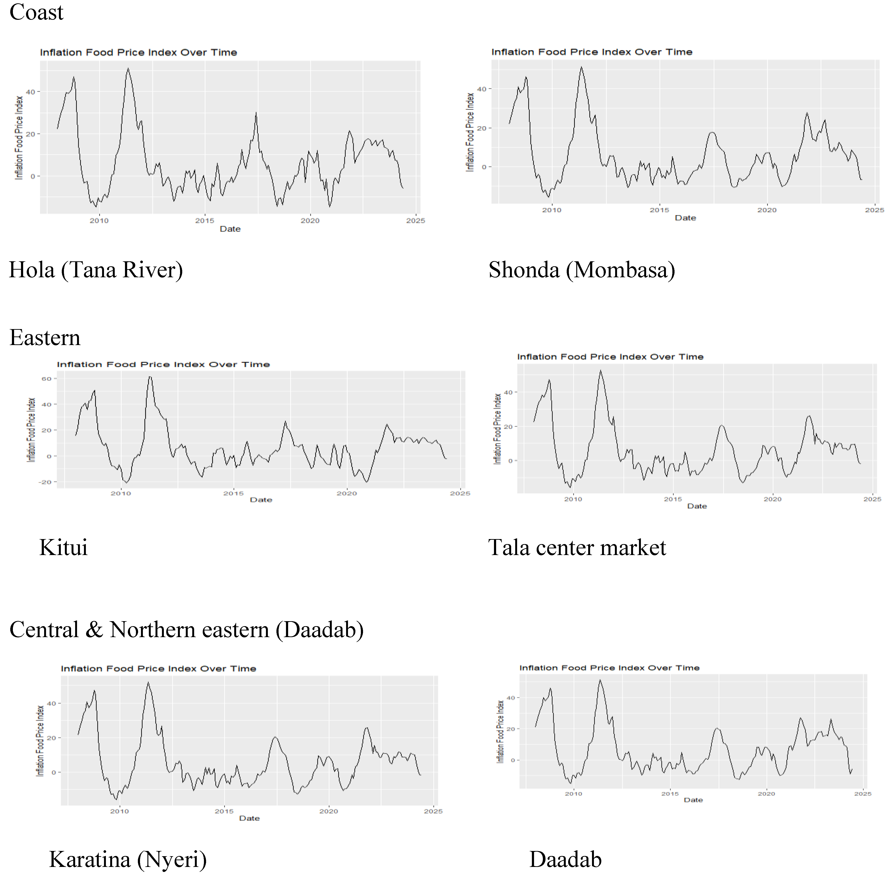
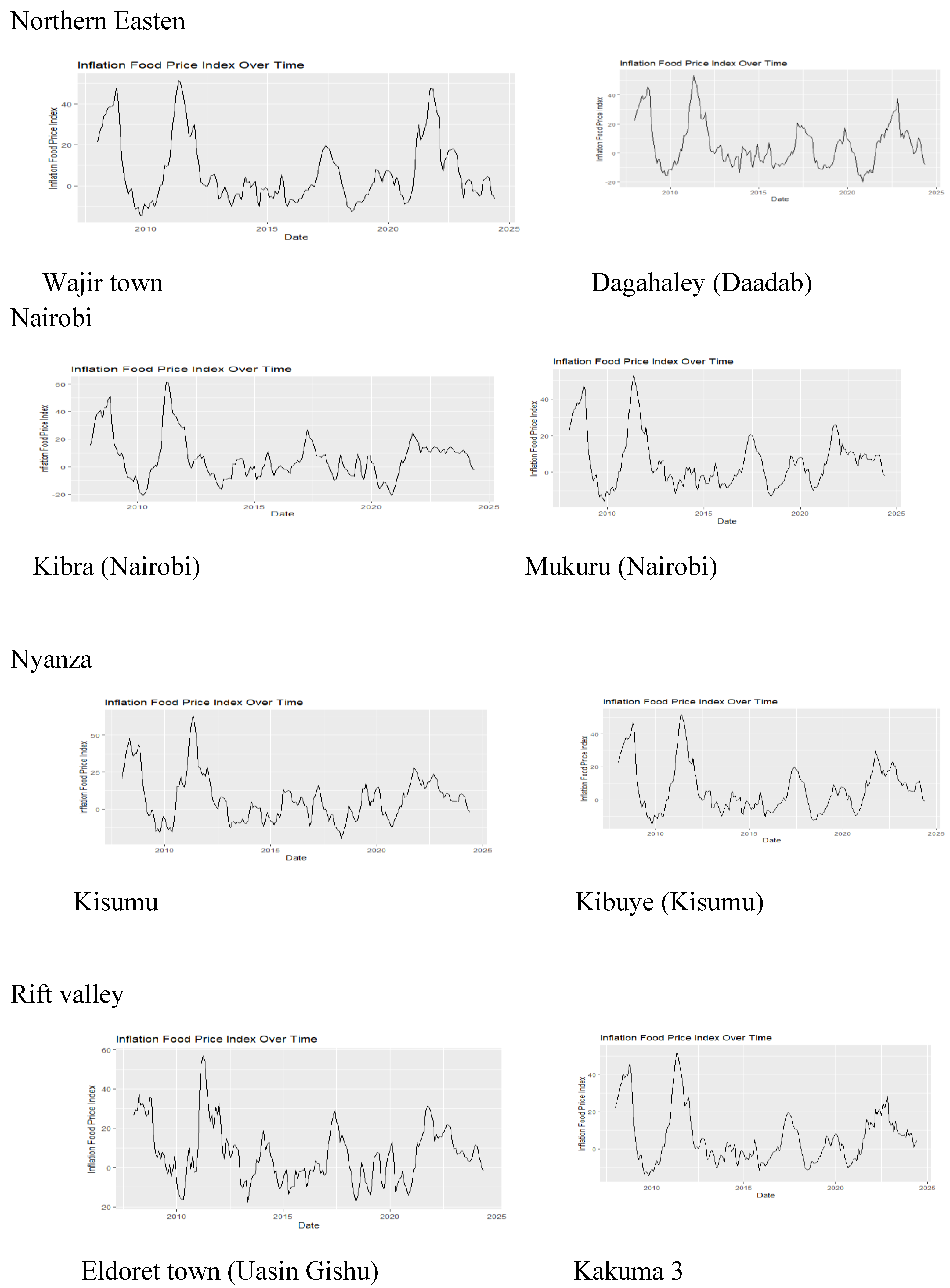
3.1. Descriptive Analysis

Table 1 below represents the desciptive analysis of selected markets in Kenya.

In Dadaab town, the lowest recorded value was -15.120, 25% of the observations were below -4.875, the middle value was 2.250, the average value was 6.507, 75% of the observations are below 14.830, and the highest recorded value was 51.630. In Dagahaley (Daadab), the lowest recorded value was -19.980, 25% of the observations were below -6.782, the middle value was 1.705, the average value was 5.347, 75% of the observations were below 13.033, and the highest recorded value was 53.540.

In Eldoret town (Uasin Gishu), the lowest recorded value was -17.750, 25% of the observations were below -3.257, the middle value was 5.180, the average value was 6.767, 75% of the observations were below 14.755, and the highest recorded value was 57.180. Hola (Tana River), the lowest recorded value was -14.890, 25% of the observations were below -3.647, the middle value was 2.315, the average value was 6.121, 75% of the observations were below 13.730, and the highest recorded value was 51.290.

Kakuma 3, the lowest recorded value was -14.590, 25% of the observations were below -5.140, the middle value was 1.430, the average value was 5.807, 75% of the observations were below 12.643, and the highest recorded value was 52.200. Karatina (Nyeri), the lowest recorded value was -16.090, 25% of the observations are below -4.780, the middle value is 1.965, the average value is 5.597, 75% of the observations are below 10.883, and the highest recorded value was 52.160. Kibra (Nairobi), the lowest recorded value was -14.970, 25% of the observations were below -4.527, the middle value was 2.475, the average value was 6.014, 75% of the observations were below 10.742, and the highest recorded value was 51.450.

Kibuye (Kisumu), the lowest recorded value was -14.300, 25% of the observations were below -4.805, the middle value was 2.280, the average value was 6.292, 75% of the observations were below 13.672, and the highest recorded value was 52.310. Kisumu, the lowest recorded value was -19.860, 25% of the observations were below -5.800, the middle value was 4.930, the average value was 6.752, 75% of the observations were below 14.825, and the highest recorded value was 62.910.

Kitui, the lowest recorded value was -20.930, 25% of the observations were below -3.868, the middle value was 4.615, the average value was 6.353, 75% of the observations were below 12.845, and the highest recorded value was 61.500. Mukuru (Nairobi), the lowest recorded value was -16.000, 25% of the observations were below -5.000, the middle value was 1.865, the average value was 5.412, 75% of the observations are below 10.360, and the highest recorded value was 50.870.

Shonda (Mombasa), the lowest recorded value was -15.670, 25% of the observations were below -4.870, the middle value was 1.900, the average value was 5.698, 75% of the observations were below 12.170, and the highest recorded value was 51.420. Tala Centre Market, the lowest recorded value was -15.920, 25% of the observations were below -4.798, the middle value is 2.035, the average value is 5.688, 75% of the observations are below 10.815, and the highest recorded value was 52.890.

Wajir town, the lowest recorded value was -14.590, 25% of the observations were below -4.875, the middle value was 1.230, the average value was 6.507, 75% of the observations were below 13.707, and the highest recorded value was 13.707.

3.2. Test for Stationarity

The Table 2 below presents the results of an Augmented Dickey-Fuller (ADF) test performed on the variables representing various towns. The ADF test is commonly used to check for the presence of a unit root, which indicates whether a time series is stationary or not [20]. A time series is stationary if its statistical properties (like mean and variance) do not change over time [21]. Most p-values were significant at the 5% level, suggesting strong evidence against the null hypothesis of a unit root, implying that the data series are stationary. In conclusion, all the variables are stationary at level (I (0)), and none of them require differencing to achieve stationarity. This implies that the data exhibits consistent statistical properties over time without a need for further transformations.

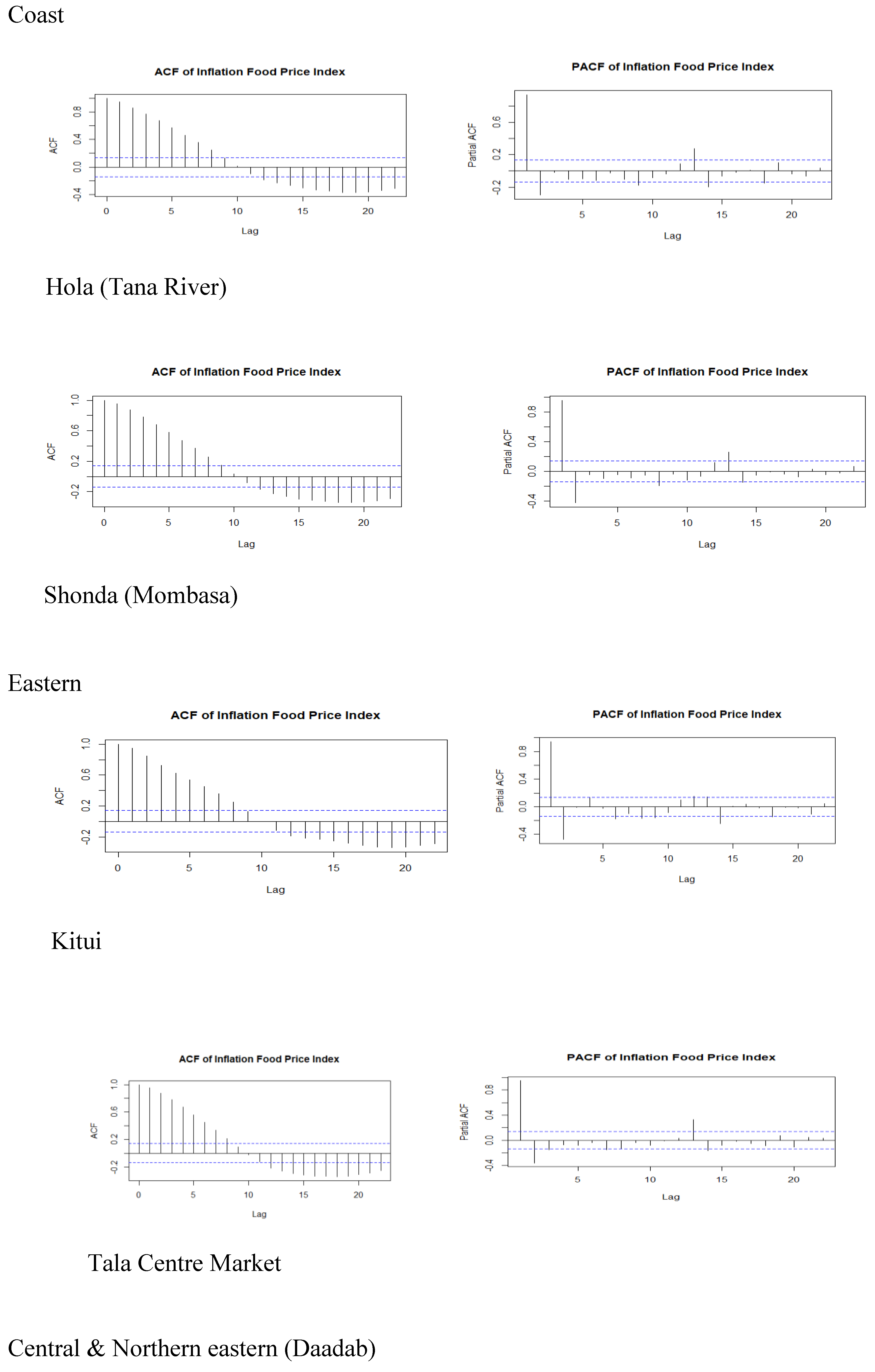
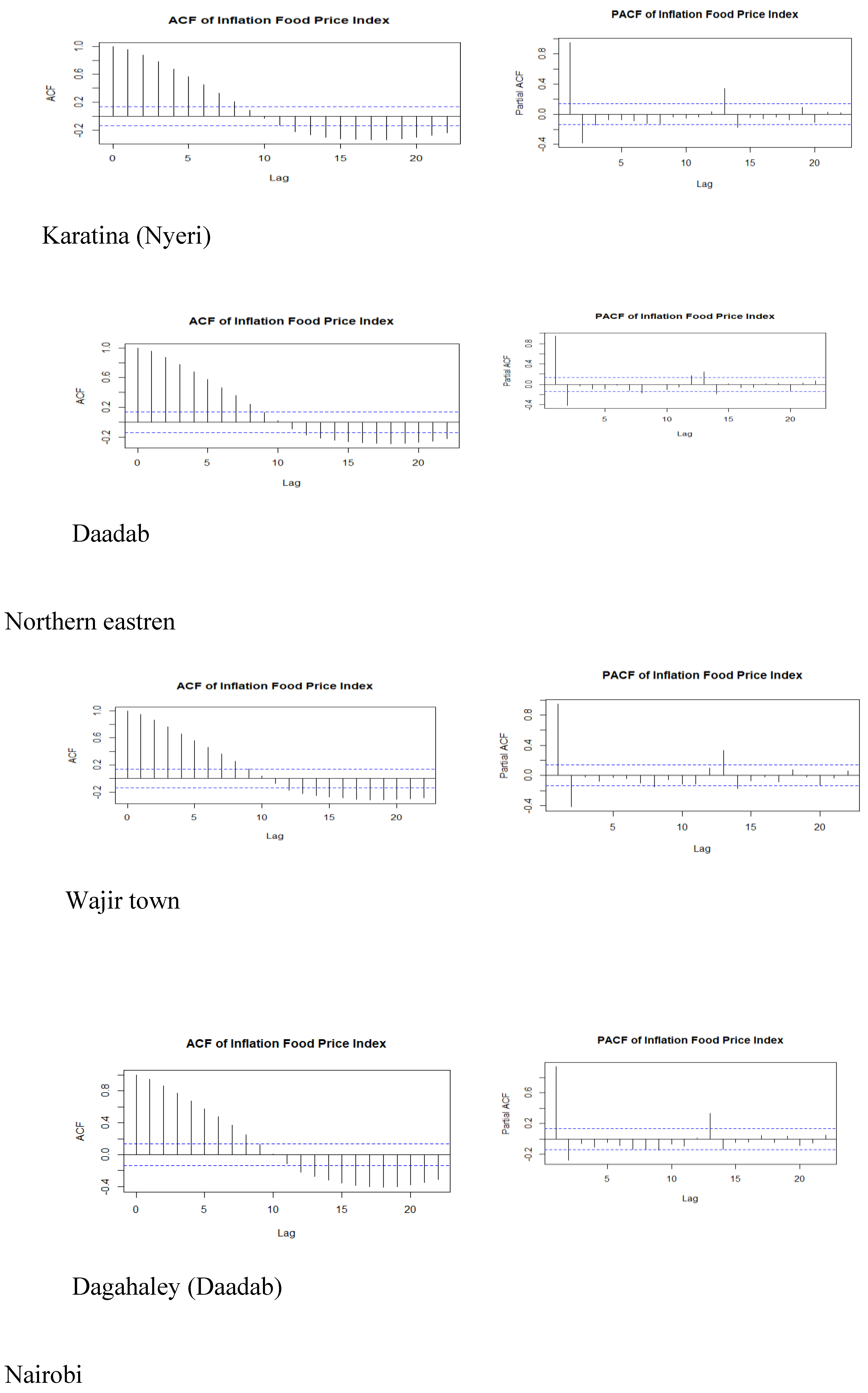
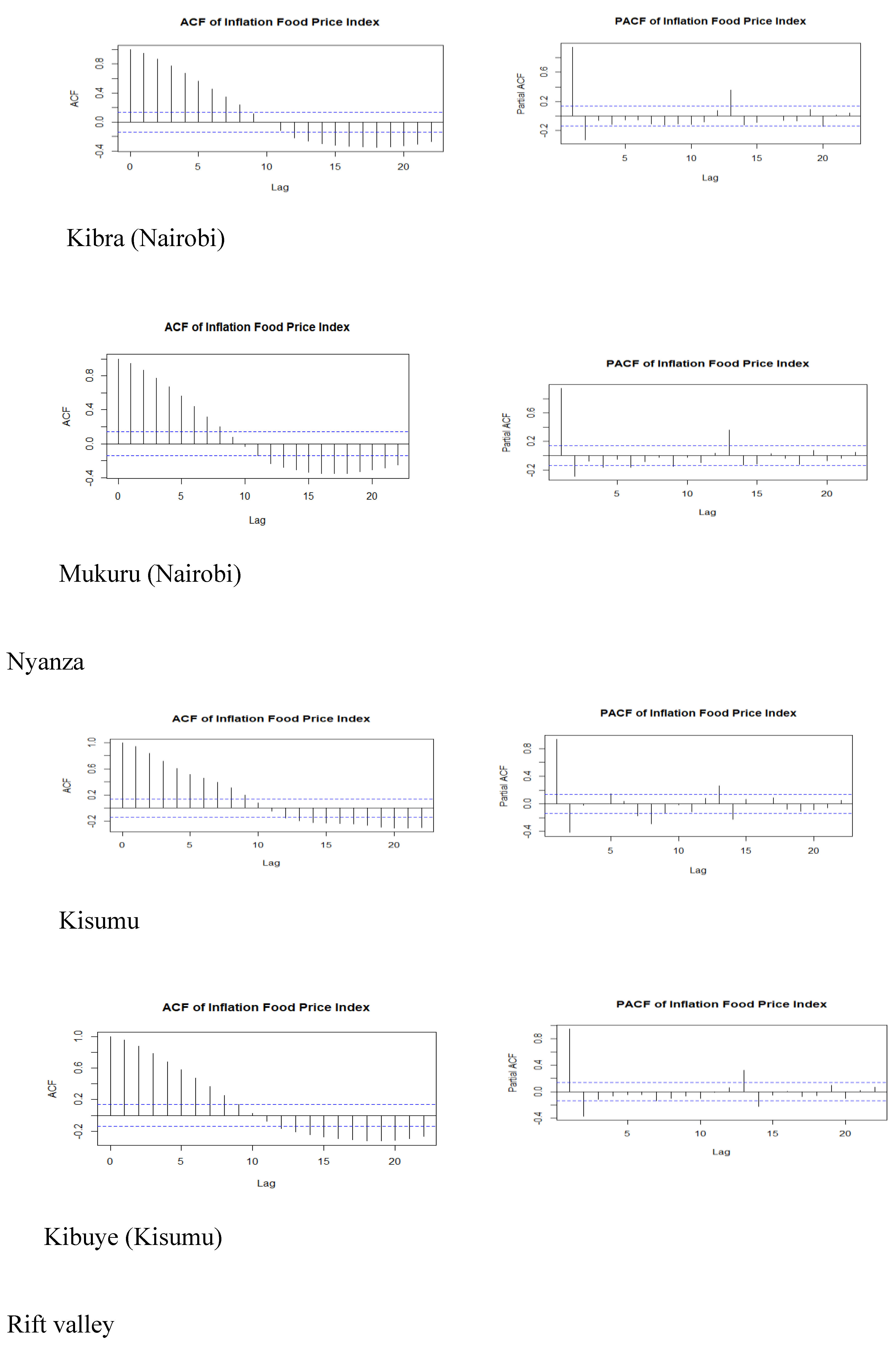
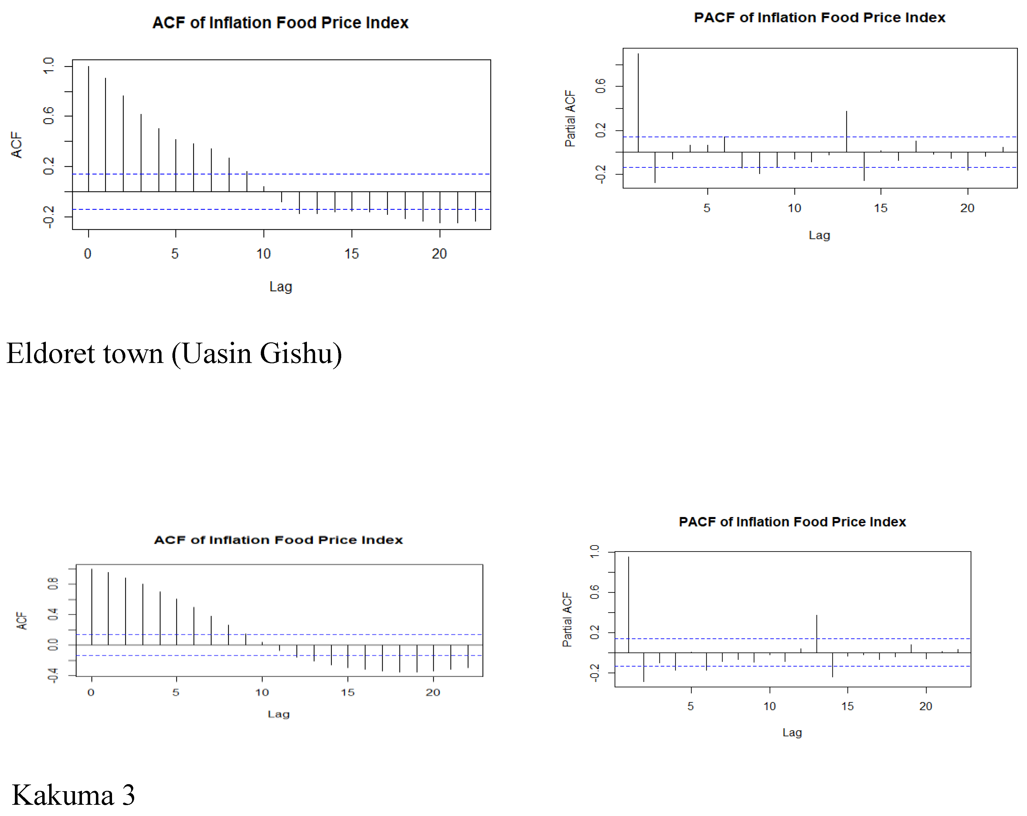
3.3. Autocorrelation (ACF) and Partial Autocorrelation Plots (PACF)

Plot Data

Figure 1 below illustrates the monthly food price index data for Kenya from January 2007 to June 2024. The pre-intervention period covers January 2007 to December 2014, while the post-outbreak period started from January 2017. As depicted in Figure below, there was a marked increase in food prices during the early stages of the 2015/16 outbreak, followed by fluctuations and eventual stabilization. The data also exhibit clear periodic and trends over the period from January 2007 to June 2024. However, all the figures indicate that the data are stationary, meaning no observable trends were present across the series. This suggests that the variables remained stable over time, without significant long-term shifts, which is essential for accurate forecasting and analysis for outbreaks on food prices index.

3.4. Autocorrelation (ACF) and Partial Autocorrelation Plots (PACF)

The ACF (Autocorrelation Function) and PACF (Partial Autocorrelation Function) graphs are key tools for determining the AR (autoregressive) and MA (moving average) components of an ARIMA model [22]. ACF helps identify MA terms by showing correlations between the series and its lags, while PACF pinpoints AR terms by isolating the direct effect of each lag. These plots guide model selection by highlighting significant lags, helping to fine-tune the ARIMA parameters for accurate forecasting. Figure 2 below shows the ACF and PACF plots of different regions used in this study

The optimal model, as shown in Table 3 below was selected by minimizing both the AIC and prediction variance. To determine the ARIMA model components, we utilized the automated auto.arima() function from the prediction package in R [23]. This algorithm systematically explores various ARIMA models to identify the one with the lowest AIC or BIC.

The auto.arima() function was applied to model inflation food price index data from January 2007 to June 2024. Following the execution of the algorithm, the best-fitting ARIMA model was identified, incorporating step and pulse changes for the respective towns.

Residual checks, as shown in the Figure 3 below, indicate a stable variance with a mean close to zero. No noticeable patterns or significant autocorrelation were detected in the residuals, suggesting that they follow a normal distribution. These findings confirm a good fit for the selected model.

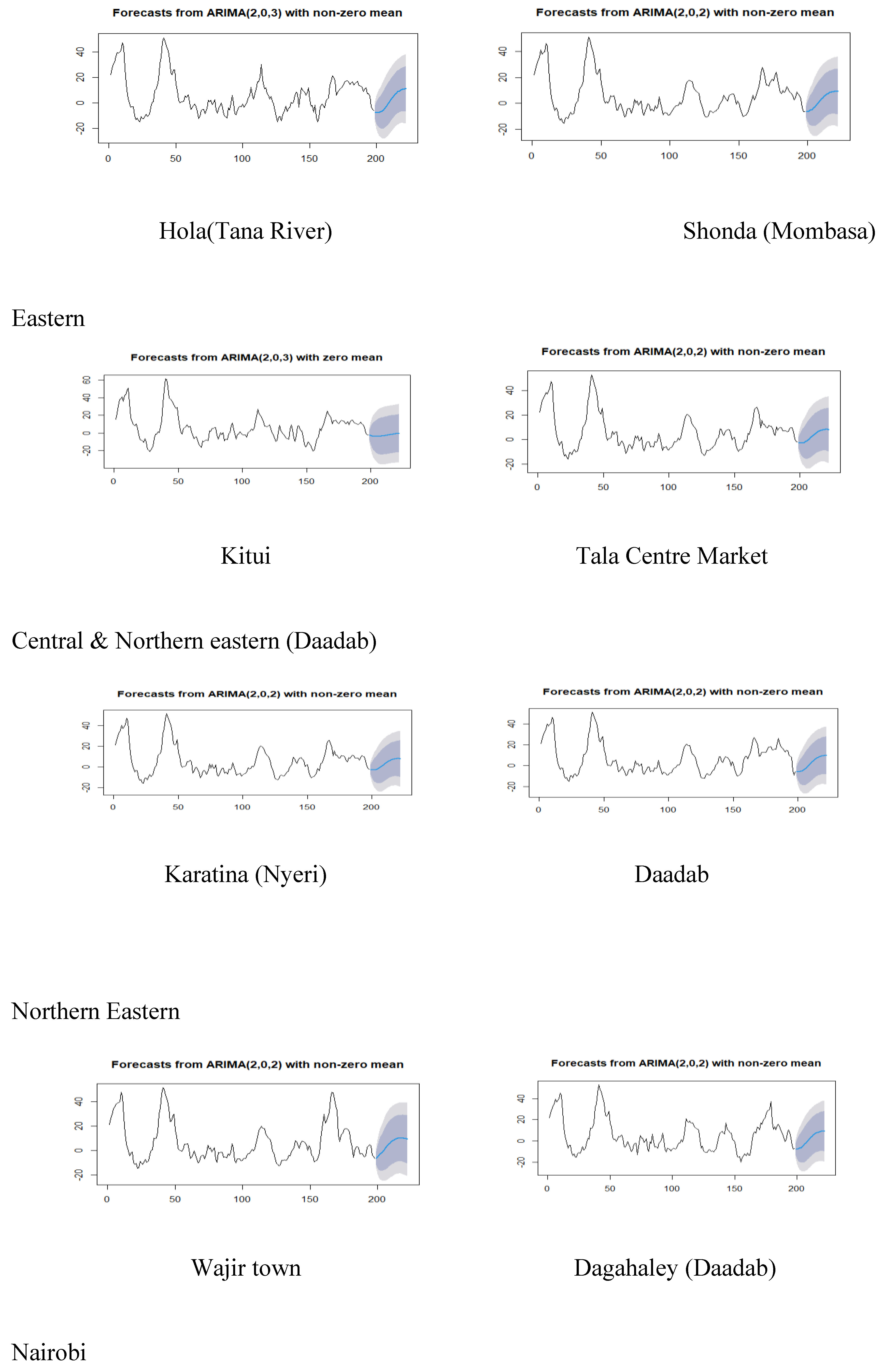
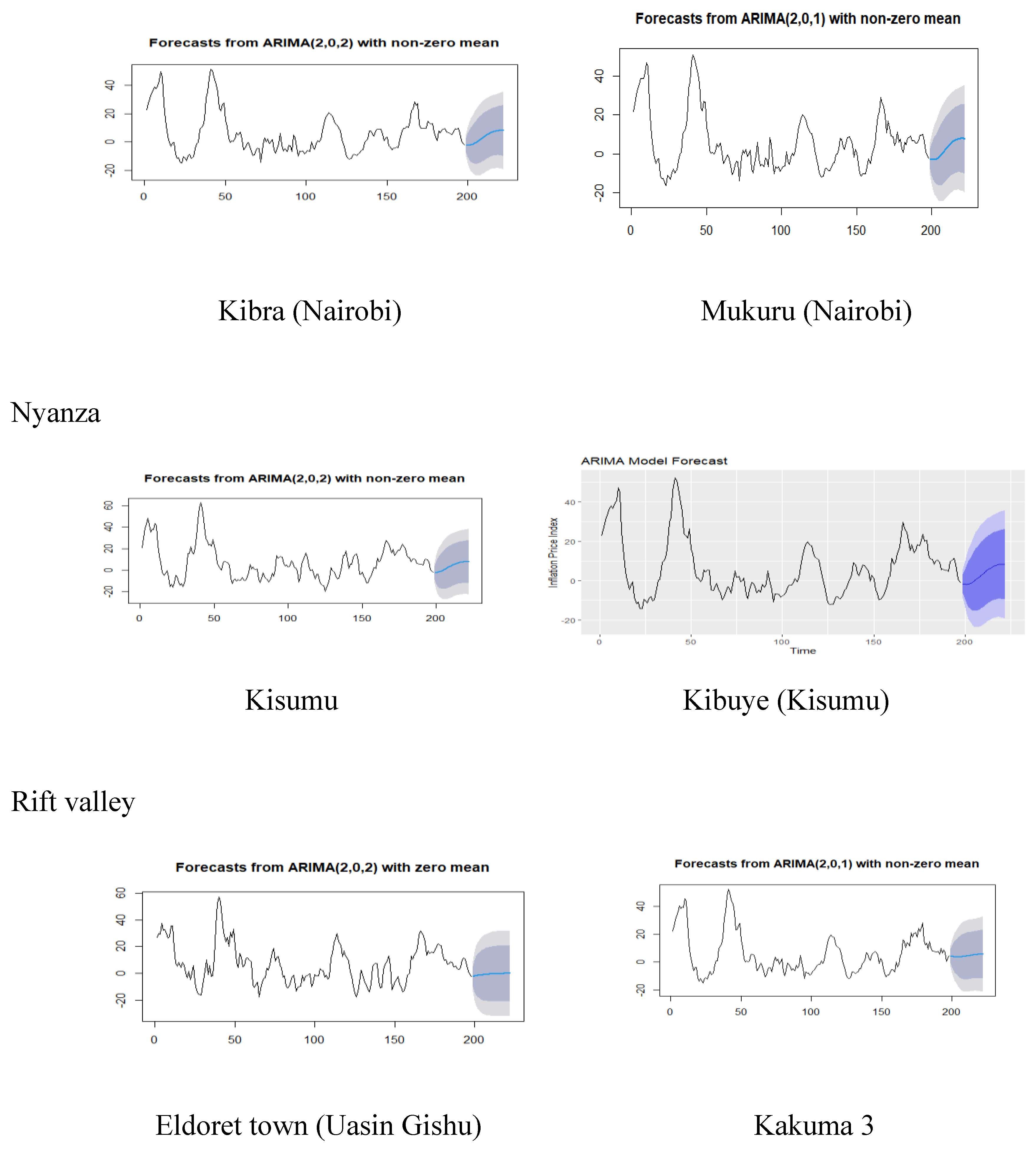
3.4. Comparison of the Forecasted and Actual Values at Various Response Levels Using the ITS-ARIMA Model from June 2018 to February 2021

The Table 4 compares the true values (actual data) and predicted values using the ITS-ARIMA model to evaluate the impact of inflation on food price indices across various markets in Kenya from June 2018 to February 2021. The absolute effect reflects the difference between the predicted and actual values, while the relative effect shows this difference as a percentage [24].

Predictions in Hola (Tana River) and Shonda (Mombasa) varied significantly, with large errors in both under- and over-estimations, especially in April 2019 and February 2021. For instance, in April 2019, Hola showed a 102.29% relative error, indicating severe model misestimation, while Shonda showed a 94.69% error. Kitui's predictions were consistently underestimated, with errors peaking at 66.75% in February 2021. Tala Centre's forecast in November 2020 had a massive 311.09% overestimation, highlighting significant volatility. Karatina exhibited extreme deviations, especially in June 2018, with a 317.18% relative error. Daadab’s predictions were more stable, with the largest relative error being 136.36% in February 2021.

Predictions for Wajir showed significant discrepancies, particularly in February 2021, where there was a 170.01% relative error. Dagahaley’s predictions were generally closer to actual values, except for November 2020, which saw an 81.99% overestimation. Kibra’s predictions were substantially underestimated in June 2018 by 397.58%, reflecting large deviations. Mukuru exhibited moderate errors, with the most significant being 88.71% in February 2021. Kisumu's forecast errors ranged from moderate to large, with an extreme overestimation of 110.98% in February 2021. Kibuye also showed large deviations, particularly in June 2018, with a 431.44% error. Predictions in Eldoret were more accurate, though there was a notable underestimation of 130.82% in April 2019. Kakuma's predictions showed moderate accuracy, with errors typically under 100%.

The ITS-ARIMA model exhibited varying prediction accuracy, with some markets experiencing large forecasting errors, especially during key periods of inflation fluctuations. The results indicate that inflation impacted different regions unevenly, and the model struggled to consistently predict these variations accurately.

Table 5 (attached in the supplementary material) displays the forecasted values for various markets in Kenya over time, focusing on different towns and markets, from July 2024 to June 2026. The values are a mix of positive and negative numbers, which reflect the predicted fluctuations in the economic or market variable being analyzed (likely related to food prices given the context).

Dadaab Town and Dagahaley, both towns begin with similar negative values in 2024, indicating a possible downturn or negative pressure on the index being measured. However, they gradually show recovery and positive growth by 2026. Kakuma 3 and Kibra (Nairobi), these towns start with positive forecasts, indicating some stability or improvement from the outset, and this continues to grow over time. However Kitui and Karatina exhibit an initial negative trend that turns positive around early 2025, suggesting a recovery from the earlier downturn.

In Eldoret Town starting with slightly negative values, Eldoret shows the smallest fluctuations among the towns, maintaining a moderate downward trend, but with smaller negative shifts than other locations. By the middle of 2025, most of the locations show positive values, with slight fluctuations around that period. The positive numbers indicate a forecast of economic improvement or market recovery in these areas. Exception in Kitui consistently records relatively high negative values in 2024 (-2.500 to -3.576), but there is a turning point in mid-2025 when the forecast starts improving. Shonda (Mombasa) started with a large negative value (-6.522 in July 2024), this town shows a steady positive improvement, reaching 9.157 by May 2026. This indicates a significant recovery or growth, perhaps linked to infrastructure or economic recovery.

Wajir Town also exhibits similar improvements, starting with -6.209 in July 2024 and recovering steadily to 9.223 in June 2026. This suggests a gradual but significant improvement. This forecasting Table projects gradual economic recovery across the towns in Kenya from mid-2024 to 2026. While most locations begin with negative values (indicating downturns or economic difficulties), there is a noticeable improvement as time progresses. By 2026, almost all towns show positive values, forecasting potential economic stability or growth across these regions. The forecasts could help policymakers and stakeholders in these regions prepare for and manage economic changes, possibly tied to food price indices or related market variables. The non-zero mean forecasts are illustrated in Figure 4.

4. Discussion

The intervention time series (ITS) analysis, with its flexibility in modeling various impacts, serves as a crucial tool for assessing the effectiveness of interventions [25]. The results unveils significant regional variability in the inflationary impact of unavoidable disruptions, such as the RVF outbreak, on Kenya’s food price index. The ARIMA model successfully identified trends in most markets, though forecast errors were notable in regions like Kisumu, Kibra, and Karatina, where inflation predictions deviated substantially from actual values. These discrepancies suggest that certain areas experienced more volatile market responses, possibly due to supply chain disruptions, market dynamics and localized economic factors

For instance, Kisumu and Kibuye showed extreme deviations, with forecast errors as high as 431%, indicating significant high volatility in food prices. This skyrocket could be attributed to the disruption of agricultural activities and transportation, especially in areas dependent on local markets. Conversely, regions like Dagahaley and Eldoret exhibited more stable trends, with relatively lower forecast errors, suggesting more resilience to economic shocks and disruptions.

These results stresses on the importance of tailored interventions to stabilize food prices across all the regions. Policymakers should prioritize infrastructure investments in volatile markets and strengthen supply chains to mitigate the impact of future disruptions. Additionally, the ITS-ARIMA model offers a valuable tool for continuous monitoring and forecasting of market trends, enabling proactive decision-making to maintain economic stability.

These findings underscore the critical role of thorough research by the regional dynamics and global organizations in shaping economic outcomes and the need for localized strategies to address inflation and food security challenges in Kenya.

5. Conclusion

In the context of our study, the ITS-ARIMA model has been utilized to evaluate the influence of RVF outbreaks on Kenya's inflation price index. This model, known for its proficiency in trend assessment and adjustment for serial correlation and seasonal impact, has been instrumental in predicting the inflation price index's trajectory, thereby providing a solid basis for effective economic strategies.

Our study indicates a consistent rise in the inflation price index since the start of outbreak in June 2018, April 2019, November 2020 and February 2021. This increase is not solely attributable to the direct effects of the RVF outbreaks but is also influenced by factors such as shifts in consumer behavior and market dynamics [26]. As we navigate the easing of restrictions, it becomes imperative to prioritize economic recovery measures and promote strategies that can effectively manage inflation and stabilize the economy. These findings provide valuable insights for policymakers and stakeholders in making informed decisions and strategies to manage inflation and stabilize the economy during and after the RVF outbreaks.

References

1. P. Bonnet, M. Tibbo, A. Workalemahu, and M. Gau, “Rift Valley Fever an emerging threat to livestock trade and food security in the Horn of Africa : a review,” Proceedings of the 9th National Conference of the Ethiopian Society of Animal Production (ESAP). 30-31 August 2001. Addis Ababa, Ethiopia. Accessed: Oct. 23, 2024. [Online]. Available: https://agritrop.cirad.fr/559463/.
2. “Food Security in an Era of Economic Volatility - Naylor - 2010 - Population and Development Review - Wiley Online Library.” Accessed: Oct. 26, 2024. [Online]. Available: https://onlinelibrary.wiley.com/doi/abs/10.1111/j.1728-4457.2010.00354.x.
3. D. Manheim, M. Chamberlin, O. Osoba, R. Vardavas, and M. Moore, Improving Decision Support for Infectious Disease Prevention and Control: Aligning Models and Other Tools with Policymakers’ Needs. RAND Corporation, 2016. [CrossRef]
4. C. Meyimdjui, “Food Price Shocks and Government Expenditure Composition: Evidence from African Countries.” Feb. 06, 2017. Accessed: Oct. 26, 2024. [Online]. Available: https://shs.hal.science/halshs-01457366.
5. M. O. Nanyingi et al., “A systematic review of Rift Valley Fever epidemiology 1931–2014,” Infection Ecology & Epidemiology, Jan. 2015. [CrossRef]
6. E. Omosa, B. Bett, and B. Kiage, “Climate change and Rift Valley fever disease outbreak: implications for the food environment of pastoralists,” The Lancet Planetary Health, vol. 6, p. S17, Oct. 2022. [CrossRef]
7. K. N. Gerken et al., “Exploring potential risk pathways with high risk groups for urban Rift Valley fever virus introduction, transmission, and persistence in two urban centers of Kenya,” PLOS Neglected Tropical Diseases, vol. 17, no. 1, p. e0010460, Jan. 2023. [CrossRef]
8. R. Espinosa, D. Tago, and N. Treich, “Infectious Diseases and Meat Production,” Environ Resource Econ, vol. 76, no. 4, pp. 1019–1044, Aug. 2020. [CrossRef]
9. I.F. P. Research Institute (Ifpri), “2011 Global Hunger Index The Challenge of Hunger: Taming price spikes and excessive food price volatility,” International Food Policy Research Institute, Washington, DC, 2011. [CrossRef]
10. “A SIMPLIFIED TIME-SERIES ANALYSIS FOR EVALUATING TREATMENT INTERVENTIONS - Tryon - 1982 - Journal of Applied Behavior Analysis - Wiley Online Library.” Accessed: Oct. 23, 2024. [Online]. Available: https://onlinelibrary.wiley.com/doi/abs/10.1901/jaba.1982.15-423.
11. J. Kisabuli, J. Ong’ala, and E. Odero, “Intervention Time Series Modeling of Infant Mortality: Impact of Free Maternal Health Care,” AJPAS, pp. 38–47, Sep. 2020. [CrossRef]
12. Y. Li, X. Liu, X. Li, C. Xue, B. Zhang, and Y. Wang, “Interruption time series analysis using autoregressive integrated moving average model: evaluating the impact of COVID-19 on the epidemic trend of gonorrhea in China,” BMC Public Health, vol. 23, no. 1, p. 2073, Oct. 2023. [CrossRef]
13. G. Chitikela et al., “Artificial-Intelligence-Based Time-Series Intervention Models to Assess the Impact of the COVID-19 Pandemic on Tomato Supply and Prices in Hyderabad, India,” Agronomy, vol. 11, no. 9, Art. no. 9, Sep. 2021. [CrossRef]
14. “MACROECONOMIC VARIABLES AND FOOD PRICE INFLATION IN NIGERIA (1980-2018).” Accessed: Oct. 26, 2024. [Online]. Available: https://ageconsearch.umn.edu/record/313621?v=pdf.
15. C. Han, “Cross-validation for autoregressive models.,” University of Louisville, 2022. [CrossRef]
16. S. Ali, S. Bogarra, M. N. Riaz, P. P. Phyo, D. Flynn, and A. Taha, “From Time-Series to Hybrid Models: Advancements in Short-Term Load Forecasting Embracing Smart Grid Paradigm,” Applied Sciences, vol. 14, no. 11, Art. no. 11, Jan. 2024. [CrossRef]
17. “Interrupted time series regression for the evaluation of public health interventions: a tutorial | International Journal of Epidemiology | Oxford Academic.” Accessed: Oct. 26, 2024. [Online]. Available: https://academic.oup.com/ije/article/46/1/348/2622842.
18. Y. K. Lee, E. Mammen, J. P. Nielsen, and B. U. Park, “Operational Time and in-Sample Density Forecasting,” The Annals of Statistics, vol. 45, no. 3, pp. 1312–1341, 2017.
19. D. G. Mayer and D. G. Butler, “Statistical validation,” Ecological Modelling, vol. 68, no. 1, pp. 21–32, Jul. 1993. [CrossRef]
20. A. Hall, “Testing for a Unit Root in Time Series With Pretest Data-Based Model Selection,” Journal of Business & Economic Statistics, vol. 12, no. 4, pp. 461–470, Oct. 1994. [CrossRef]
21. .
22. “Autocorrelation and partial autocorrelation functions to improve neural networks models on univariate time series forecasting.” Accessed: Oct. 23, 2024. [Online]. Available: https://ieeexplore.ieee.org/abstract/document/6252470.
23. T. M. Awan and F. Aslam, “Prediction of Daily Covid-19 Cases in European Countries Using Automatic Arima Model,” Journal of Public Health Research, vol. 9, no. 3, p. jphr.2020.1765, Jul. 2020. [CrossRef]
24. M. Noordzij, M. van Diepen, F. C. Caskey, and K. J. Jager, “Relative risk versus absolute risk: one cannot be interpreted without the other,” Nephrology Dialysis Transplantation, vol. 32, no. suppl_2, pp. ii13–ii18, Apr. 2017. [CrossRef]
25. S. Gilmour, L. Degenhardt, W. Hall, and C. Day, “Using intervention time series analyses to assess the effects of imperfectly identifiable natural events: a general method and example,” BMC Med Res Methodol, vol. 6, no. 1, p. 16, Dec. 2006. [CrossRef]
26. Y. Li, X. Liu, X. Li, C. Xue, B. Zhang, and Y. Wang, “Interruption time series analysis using autoregressive integrated moving average model: evaluating the impact of COVID-19 on the epidemic trend of gonorrhea in China,” BMC Public Health, vol. 23, no. 1, p. 2073, Oct. 2023. [CrossRef]
Figure 1. Monthly food price index.
Preprints 140473 g001aPreprints 140473 g001b
Figure 2. ACF and PACF plots.
Preprints 140473 g002aPreprints 140473 g002bPreprints 140473 g002cPreprints 140473 g002d
Figure 3. Residual checks.
Preprints 140473 g003aPreprints 140473 g003b
Figure 4. The non-zero mean forecasts.
Preprints 140473 g004aPreprints 140473 g004bPreprints 140473 g004c