Submitted:
24 November 2024
Posted:
25 November 2024
You are already at the latest version
Abstract
Airborne LiDAR point cloud data, as a commonly used spatial data, is also the main source for obtaining high-quality Digital Elevation Model (DEM) at present. In order to study the relationship between point cloud data and interpolation algorithms under different sampling densities on the accuracy of DEM construction, and to verify that the test area can form high-quality DEM topographic maps in 1:500 and 1:1000 large-scale topographic maps to meet the mapping standards, this paper uses airborne point cloud data under flat and gully terrain conditions as the experimental objects. Firstly, the KD tree is constructed to find the effective point cloud according to the distance threshold, in order to further enhance the filtering effect, the bilateral filtering factor is used to determine the noise points to achieve multi-scale denoising, and then the fabric filtering algorithm is used to find the seed points to achieve the accurate separation of the ground points from the non-ground points; secondly, the ground point data are randomly sampled into different densities, and the ground point data are randomly sampled into different densities by establishing a spatial interpolation algorithm (Kriging (Ordinary Kriging, OK), Radial Basis Function (RBF), and Inverse Distance Weighting (IDW) to generate DEMs at different densities, and use the root-mean-square error for accuracy assessment. The results show that: 1. The accuracy of the DEM generated by the interpolation algorithm all decreases with the reduction of the point cloud density, and the accuracy of different interpolation algorithms is obviously different, when the sampling rate reaches 50% OK and IDW accuracy is optimal, the topographic features are clearly characterised and the RBF accuracy is the lowest; 2. With the enhancement of the density of point cloud on the ground, the level of accuracy of the DEM tends to be gradually stabilised. When the sampling density reaches below 30%, the DEM accuracy decreases linearly.
Keywords:
LiDAR
; digital elevation model
; point cloud filtering
; point cloud density
; spatial interpolation
1. Introduction
With the continuous development of China's smart mines, mining and construction by the traditional industry to modernise the industry transformation and gradually towards intelligent intelligent mines, mine monitoring the degree of refinement continues to improve, and accordingly to the mine survey workers also put forward higher requirements [1,2,3,4,5].Most of the mining in our country is in the remote mountainous areas, due to the complex environment, poor conditions and other factors that lead to mine surveying staff work is extremely difficult, in the steep slopes and valleys in the measurement, personnel and equipment safety can not be guaranteed, and therefore in the terrain of the village section is also prone to all the trouble is not suitable to carry out the work of surveying. Digital Elevation Model (DEM) is a form of digitally describing the elevation information and thus representing the ground surface [6,7,8,9]. As the basic data for remote sensing geomorphological analysis and simulation, DEM is widely used in Geographic Information System (GIS), remote sensing, geological research, urban planning, real-image three-dimensional, flood prediction and water resources, The traditional methods of obtaining DEMs are mostly ground surveys and aerial photogrammetry, but in recent years, with the rapid development of remote sensing technology and LiDAR (Light Detection and Ranging), it has become the main source of high-quality DEMs by virtue of its high-precision data acquisition [14,15,16].
Nowadays, the state actively promotes the low altitude economy to use the field to carry out multi-scenario applications [17,18,19], the rise of UAV and photogrammetry technology can be well applied to the field of mines, the use of three-dimensional spatial surveying technology to measure and process the terrain of mines, which greatly reduces the burden of the external operators; Chen Bangsong [20] and others proposed an optimal collection point density calculation method based on local terrain complexity and discrete difference peak-finding method, and investigated the optimal point density at different scales and depression degrees, but the applicability in different regions and geological conditions is yet to be verified, and the selection of the optimal scale still lacks systematic research; Bei Yixuan [21] studied and evaluated the impact of airborne LiDAR point cloud density and interpolation methods on the accuracy of digital elevation model (DEM) and surface roughness in three regions with different terrain features; Liu Yicheng [22] and others used random sampling algorithm to thin the point cloud data in the mountainous area of Yongxing Township, Huaping County, Yunnan Province, for the complex mountainous terrain conditions under different point densities, and carried out DEM modelling and accuracy assessment for them, and the point cloud retention rate was positively correlated with the DEM accuracy, but there were fewer studies on further refinement of the complex terrain, and other factors that might affect the accuracy of the DEM were not taken into account; By selecting two types of terrains, flat and mountainous, as the test area, Xiao J. [23] et al. used an irregular triangular mesh-based point cloud thinning algorithm to thin the ground point cloud data with different retention rates and assessed the accuracy of the generated DEMs; Zhang Hongyue [24] study combines the advantages of two algorithms, progressive encrypted triangular mesh filtering and fabric simulation filtering, through the noise point constraints and seed point selection and other steps to effectively remove the noise points in the point cloud data, compared with a single filtering algorithm, the error is significantly reduced accuracy is higher, however, in the study of the applicability to the complex region needs to be further optimised; Yuan Zhuang [25] and others studied and verified the feasibility of the application of UAV 3D laser scanning technology in the mining area under the complex terrain conditions, and put forward the application method of UAV 3D laser scanning technology in the mining area for the rock shift observation, but there are limitations in the separation of ground point and non-ground point methods in the filtering of low vegetation, and the measurement accuracy needs to be further optimised in order to reduce the systematic error; Zhou D [26] and others validated the method of monitoring subsidence in coal mine area by combining GPS and terrestrial three-dimensional laser scanner (TLS) technology, but due to the high operational complexity, further optimisation of the algorithm and process is needed to improve the efficiency, and the alignment error of the point cloud data may still affect the monitoring results, which is yet to be improved in the alignment algorithm; Hao J [27] used unmanned aerial digital photogrammetry (UAV-DP) technology to acquire high-resolution images, used structure-from-motion algorithms to construct a 3D point cloud model of the slope surface, performed coplanarity detection and K-means clustering to identify the structural surfaces, and finally analysed the slope's stability and instability modes by stereographic projection and discrete element methods, but the insufficient density of the studied point cloud may lead to fineinaccurate identification of structural surfaces, which affects engineering applications; Meng X [28] proposed a multilayer adaptive filtering (MAF) algorithm based on morphological reconstruction and thin-plate spline interpolation for airborne LiDAR point cloud filtering, which ultimately achieves effective filtering of complex terrain by stepwise generating a digital elevation model, extracting the ground pixels using morphological reconstruction and compensating the residual thresholds according to the terrain gradient, but the selection of the initial ground seed has a significant impact on the filtering of theresults to be optimised, and the propagation effect of misclassification is considered in the subsequent iteration process to reduce the commissioning error; Li F [29] proposed a multilevel adaptive surface interpolation filtering method based on fabric simulation and terrain amplitude, which generates initial ground seed points by multilevel temporary digital elevation model raster surfaces and thin-plate spline interpolation combined with a fabric simulation algorithm, and sets the residual thresholds adaptively using terrain amplitude, thus achieving the capture and accurate classification of complex terrain features, but in the case of the complex terrain features containing a large number ofoutliers, complex regions still have high misclassification; Lian X [30] and others used terrestrial laser scanning technology to monitor and analyse the ground hazards in the Gaoyang coal mine in Shanxi, performing point cloud data acquisition, modelling and spatial analysis, and comparing it with the total station monitoring method, but there are limitations in obtaining absolute displacement data.
Aiming at the above problems, this paper selects two different terrains as the test area, in order to verify that the test area can form high-quality DEM topographic maps in 1:500 and 1:1000 large-scale topographic maps to meet the cartographic standards, the airborne LiDAR point cloud data is used as the data source, and the commonly used interpolation algorithms are used to streamline the point clouds of these four groups (the streamlined point counts of the original point cloud counts of 90%, 70%, and 50%,30%) were interpolated to construct DEM data at different scales, and their accuracy and the generated shadow maps were analysed and evaluated, aiming to provide a more comprehensive understanding for the subsequent construction of high-precision DEMs.
2. Study Areas and Data
2.1. Study Area
The study area of this experiment is located in the Tinnan Coal Mining Area in Changwu County, Xianyang City, Shaanxi Province (34°59′39″–35°18′44″N, 107°38′53″–107°58′20″E), as shown in Figure 1. This region lies within the gully-dominated section of the Loess Plateau in northern Weihe River, characterized by complex terrain and rugged roads. The loess tablelands have steep slopes and loose surface soil. The topography of the Tinnan Coal Mine predominantly features typical loess remnants and gully landforms. From an aerial view, the loess tablelands often appear petal-shaped. The top surfaces of these tablelands are generally flat, with slopes ranging from 1° to 3°, and edges reaching up to approximately 5°. The area is surrounded by deeply incised valleys, with the highest elevation being 1,194 m (Hulin Village) and the lowest at 850 m (Heihe River in Tingbei Village), resulting in a maximum elevation difference of 344 m and a relative elevation difference of 200 m between tablelands and gullies. The geomorphic conditions make topographic surveying and surface movement monitoring challenging within the mining area. The ecological and geological environment of the mining area is highly fragile, with scarce water resources and an average vegetation coverage of approximately 15%, mainly consisting of xerophytic plants. The annual precipitation ranges between 400 and 500 mm, concentrated mainly in June to August, which accounts for 70-80% of the total yearly rainfall. The area experiences strong winds and frequent dust storms, indicative of a typical arid to semi-arid climate.
2.2. Data Acquisition and Preprocessing
The point cloud data collected by the VSurs-L-UMR UAV laser scanning system developed by Qingdao Xiushan Mobile Measurement Co. Ltd. was selected for this pilot study, carrying a multi-rotor UAV carrier platform with highly integrated high-performance sensors such as a satellite positioning receiver (GNSS), a laser scanner (LiDAR), an inertial measurement unit (IMU), and an industrial camera (CCD). The vehicle over the study area has an altitude of 600-800m, a speed of 8m/s, a scanning angle of ±36°and a laser pulse of 600kHz.The horizontal/vertical positioning accuracy of the surface points of the LiDAR system is 0.1 m/0.03 m, respectively.The obtained point cloud data consists of two parts: a low-density point cloud and a high-density point cloud (Figure 1-d), and the raw point cloud acquisition information is shown in Table 1.
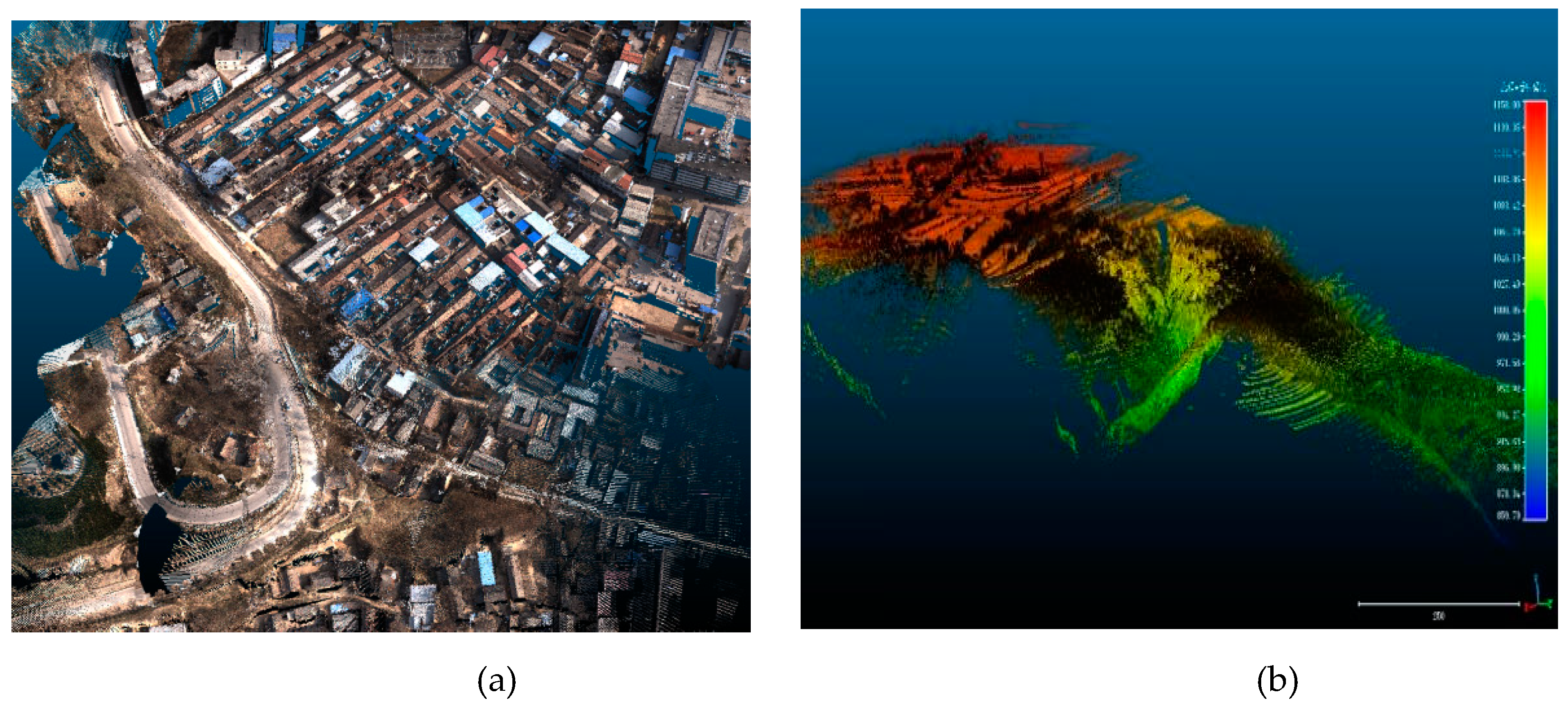
Figure 2.
Point cloud data under flat terrain and gully terrain conditions: (a) Flat terrain; (b) Gully relief.
Figure 2.
Point cloud data under flat terrain and gully terrain conditions: (a) Flat terrain; (b) Gully relief.
3. Methodology
This section may be divided by subheadings. It should provide a concise and precise description of the experimental results, their interpretation, as well as the experimental conclusions that can be drawn.
3.1. Combinatorial Filtering Algorithm Based on Multiple Conditions
In addition to the constraints of removing noise points from the original point cloud data, this paper proposes a filtering method that firstly takes into account the influence of the selection of seed points, and then uses the fabric filtering algorithm to identify seed points with the progressive encrypted triangular mesh filtering method for the iterative identification of the ground points, which constrains the seed points to form a new combined filtering algorithm.
As shown in Figure 3-(b),the original point cloud will be constructed KD tree to search for noise points in accordance with the set distance threshold to confirm whether it is a valid point cloud, after which the bilateral filtering factor is used to determine the noise points so as to realise the noise removal through the large scale and small scale; subsequently, the fabric filtering algorithm is used to search for the seed point location to obtain the seed point, and the establishment of the structure with triangular mesh for the encryption of the network to carry out the calculation of the remaining points, and at the same time should take into account the distance between the to-be-seeked points and the structure of the network and theangle, when the corresponding threshold conditions are met, the point can be judged as a ground point, thus completing the encrypted triangular mesh.
In the progressive triangular mesh filtering processing of point clouds, it is necessary to judge the spatial location of the point cloud in order to construct the triangular mesh and encrypt the subsequent triangular mesh, so the parameters are relaxed in the selection of the seed points, and the spline interpolation algorithm is introduced to obtain accurate ground seed points using the seed point identification in the fabric filtering method.
The advantage of the thin-plate spline interpolation method is that it can achieve a distribution of points within a region using a limited number of reference points, and even if the reference points are sparse, it can still generate a high-quality interpolated surface. Meanwhile, in order to prevent elevation anomalies from adversely affecting the interpolation function, regularised thin-plate spline interpolation is introduced when it is not possible to ensure that the initial seed points are completely accurate. By adjusting and modifying the coefficients of the regularisation terms, the degree of deformation of the interpolated surfaces can be effectively adjusted to simulate the topography more realistically and to reduce the influence of low-quality interpolation points. The TIN is constructed through the point cloud data of the survey area, and the ground point cloud is obtained according to the processed point cloud, based on which an irregular triangular grid is generated through a series of points, and the triangular grids are connected with each other to form a kind of spatial three-dimensional structure, thus forming a digital elevation model.There are two main types of common irregular grid construction Voronoi diagram and Delaunay grid construction, both of which are used to analyse the area through the use of discrete data, and are currently commonly used grid construction algorithms.
3.2. Establishment of DEM Interpolation Algorithm
When generating a digital elevation model, the parameters of raster cell size, in the x-direction and y-direction resolution, are required to be set, and the interpolation method used to determine the raster cell size, requires a certain buffer to be set, in terms of the grid. The DEM is extracted based on ground point interpolation algorithms, generally using inverse distance weighting algorithm, radial basis function interpolation algorithm, kriging interpolation algorithm.
(1)Inverse distance weighting algorithm
Inverse distance weighted interpolation algorithm is a spatial interpolation algorithm, spatial neighbouring sample points to the estimation of the point of the influence of the distance increases and decreases, the size of the weight is related to the distance between the sampling point and the interpolation point, the algorithm is essentially similar for the weighted average method, the first step is to specify the value of the weights of each sample point, and then multiply with the value of the individual sample points and sum up to get the overall value, and then divided by the sum of the weights of the individual sample points [31].sum of the weights of each sample point [31].Assuming that Zi is the value of the known sample point, Pi is the corresponding weight value of the known sample point, and Zp is the value of the interpolation point to be sought, it is calculated according to the following formula:
The value of the weights in the inverse distance weighting is determined by the following equation:
where, di is the distance between the interpolated point and the known point; u is the weight index, i.e., the control parameter, the larger the value of u, the weight decreases with the increase of the distance; usually u takes 1-3.
(2) Radial Basis Function Interpolation Algorithm
Radial basis functions are a mathematical method used for interpolation and regression to generate continuous elevation surfaces using elevation values at discrete points when constructing terrain modelling and digital elevation models. The RBF is a distance-dependent function, the value of which depends on the distance between some centre point and the input point, and is commonly of the form ; where x is the position of the input point (the position to be interpolated) and c is the centre point (the elevation value of the known point), is the Euclidean distance (or other measure) between the input point and the centre point.
is the radial basis function, commonly used radial basis functions are generally Gaussian function, binomial function, thin plate spline function and so on. Then an interpolation function is built based on the discrete points to estimate the elevation value of any point. This interpolating function is usually a weighted sum form of a known radial basis function:
where is the weight to be sought, is the elevation value of the known discrete points, and is a polynomial to deal with the global trend; a system of linear equations is constructed to solve for the weights by using the known elevation data points, and finally an interpolation function is used to compute the elevation value of each raster in the target area, thus generating a continuous elevation surface. The elevation value of each raster point is inferred from the neighbouring known points by the number of interpolated values.
(3) kriging interpolation algorithm
The DEM model is built by interpolating the regional data through the optimal interpolation estimation, which is more adaptable to the regions with distinctive terrain undulation features. This interpolation algorithm is mainly embodied in estimating the attribute values of the point cloud in the space.
For any point (x, y, z) on the space, which can be expressed as z=(x, y), the required interpolation point attribute value is Z(x0), then the attribute value of any point is Z(xi), and the result obtained by using the Kriging Interpolation algorithm is that Z*(x0) is the weighted sum of the attribute values of the known sampling points, Z(xi), that is:
where λi is the pending weight coefficient, determine the criteria for the selection of the pending weight coefficient λi to obtain the unbiased optimum satisfies the following function:
E[Z(x)] is known to be a constant and can be found from the above equation:
The relation can be derived:
Estimating the minimum variance is obtained:
Obtained by applying the Lagrange multiplier method of conditional extremes:
Among them, , a system of linear equations of order n+1, known as the Kriging system of equations, is obtained by further derivation and is publicised as follows:
Among them, is the covariance function of Z(xi) and Z(xj).
3.3. DEM Accuracy Evaluation Index
The commonly used accuracy evaluation metric, Root Mean Square Error (RMSE), is defined by the following formula:
In the formula, Zi represents the elevation value at sampling point i; z represents the elevation value at checkpoint i; and n denotes the number of checkpoints. Let .
4. Results and Discussion
4.1. Result Analysis of Combined Filtering Algorithm
4.1.1. Qualitative Analysis
To evaluate the effectiveness of filtering, both qualitative and quantitative analyses are commonly used to assess the quality of the filtering results, thereby determining the feasibility of the method.
Figure 4.
The section effect of each filter algorithm:(a) Planar topographic map;(b) Actual topographic profile of the original point cloud;(c) Ground points;(d) Fabric filtering algorithm terrain filtering effect profile;(e) Ground points;(f) Progressive triangulation filter terrain filtering effect profile;(f) Progressive triangulation filter terrain filtering effect profile;(g) Ground points;(h) Combined filtering algorithm terrain filtering effect profile.
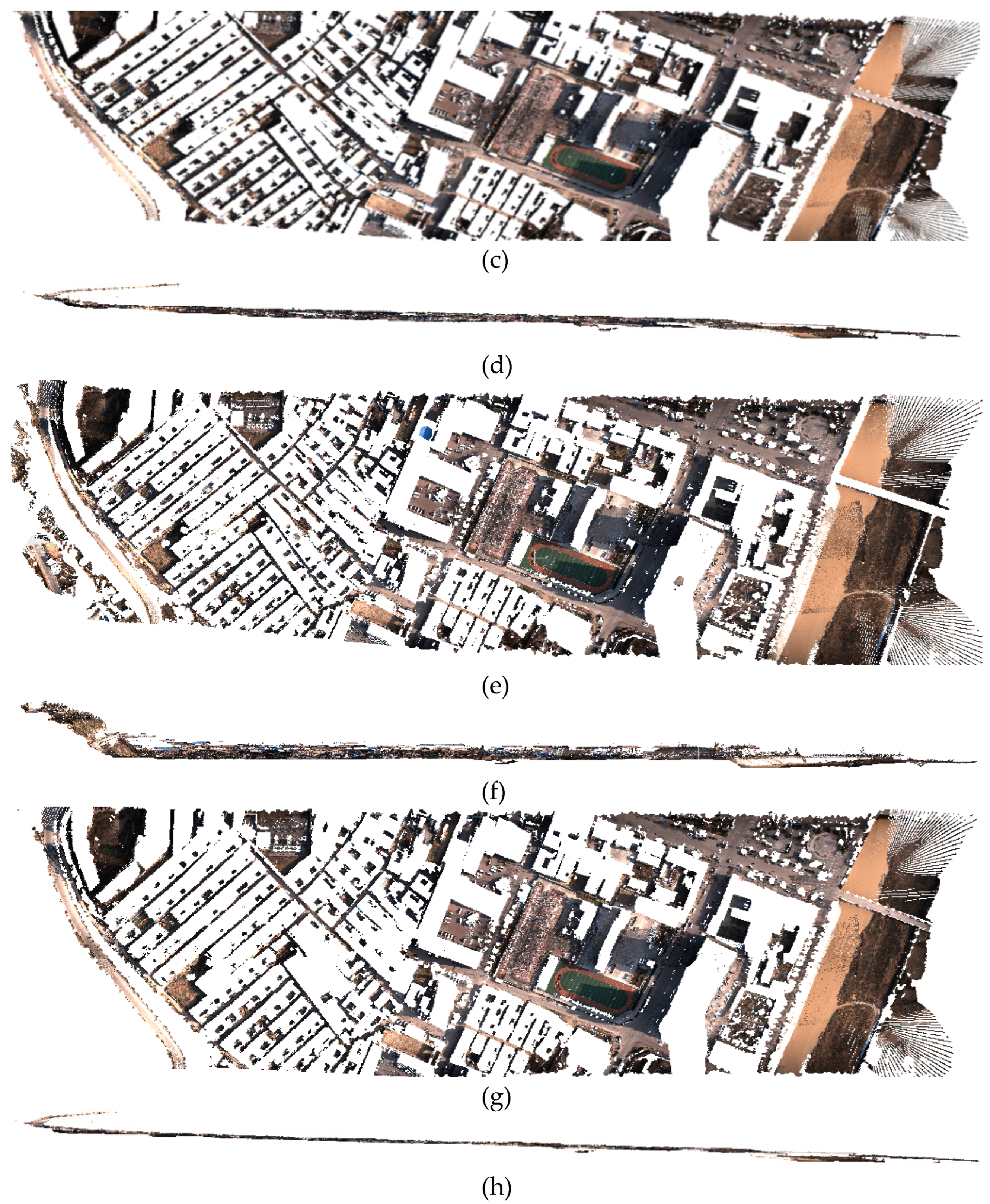
From the profile data obtained after filtering, the quality of the filtering results can be assessed to evaluate the performance of different algorithms. As shown in the figure, for flat terrain areas, the progressive triangulated irregular network (TIN) filtering algorithm exhibits incomplete removal of non-ground points, with some non-ground points mistakenly classified as ground points. This issue arises due to suboptimal parameter selection, particularly in angle settings. In contrast, both the cloth simulation filtering algorithm and the combined filtering algorithm show better filtering performance. Additionally, the combined filtering algorithm is able to preserve more ground points, further enhancing its effectiveness.
4.1.2. Quantitative Analysis
In order to analyse the magnitude of the accuracy of the filtered ground point cloud, it can be judged according to the cross-tabular evaluation system [32], which takes into account the precise determination of the number of correctly classified and incorrectly classified points after the filtering, with correctly classified points divided into ground and non-ground points, denoted as a and d, and incorrectly classified points with incorrectly classified non-ground points and incorrectly classified ground points, denoted as b and c. According to the structure in the cross-tabulation, the errors in point cloud filtering can be classified into three categories: one type of error, also called according to the truth error, denoted as Error1, which indicates the probability that a ground point is misclassified as a non-ground point; two types of error, also called nano-pseudo error, denoted as Error2, which indicates the probability that a non-ground point is misclassified as a ground point; and the total error, denoted as Error, which indicates that the classification effect is not in agreement with the reference data of theprobability; and thus a quantitative analysis of cross judgement based on the number of points.

Table 2.
Accuracy evaluation table of ground filtering algorithm.
| Terrain Data | a | b | c | d | Error1 | Error2 | Error |
|---|---|---|---|---|---|---|---|
| Flat Terrain | 7611447 | 42365 | 8562 | 4031680 | 0.55 | 0.21 | 1.26 |
| Ravine Terrain | 18451578 | 3528642 | 485642 | 16735268 | 16.05 | 2.82 | 10.24 |
From the above table, it can be seen that for the flat terrain filtered data, the first class error is 0.55 per cent, the second class error is at 0.21 per cent, and the total error is 1.26 per cent; for the gully terrain data, the first class error is 16.05 per cent, the second class error is at 2.82 per cent, and the total error is 10.24 per cent; from the table, it can be seen that the second class error is smaller. The greater density of surface points leads to a smaller impact of a class of errors, which shows that the algorithm is more suitable for filtering processing of surface deformation observations in mining areas.
4.2. Analysis of DEM Results Formed at Different Cloud Densities
4.2.1. Selection of Point Cloud Density
By constructing a digital elevation model, the elevation information of the surveyed area can be directly observed and analysed, which is a very important part of the survey results.3D laser point cloud data contains a huge number of measured points and the elevation information of these points is usually also very rich, which leads to a large amount of computation when generating a digital elevation model (DEM).Even with proper streamlining of the point cloud data, the dataset will still contain a large number of elevation points. In the actual process of generating the DEM, the large amount of point cloud data will put high demands on the computer and require a long computing time.
If the generated DEM model can still maintain a high accuracy after properly streamlining the point cloud data, it will be easier to handle and manipulate the 3D elevation point data in actual production. Therefore, a reasonable point cloud density needs to be selected in the process of generating the DEM to ensure the accuracy of the DEM.
Table 3.
Overview of the Raw Point Cloud Data.
| Resampling Percentage | Number of Flat Terrain Point Clouds | Average Elevation/m | Number of Point Clouds in Gully Terrain | Average Elevation/m |
|---|---|---|---|---|
| 90 | 3628512 | 867.71 | 15061742 | 1125.84 |
| 70 | 2539958 | 865.52 | 12049394 | 1125.71 |
| 50 | 1814256 | 862.63 | 9037045 | 1125.03 |
| 30 | 1088553 | 858.90 | 6024696 | 1124.07 |
| 10 | 362851 | 854.12 | 1506174 | 1102.36 |
According to the idea proposed by Heng [33], the optimal grid resolution for constructing the DEM is halfway between the point spacing, so before studying the interpolation method chosen in the region, to analyse the effect of different sampling densities on the accuracy of the DEM, the original point cloud data were randomly sampled at 90%, 70%, 50%, and 30% of the full density, and the density conditions are shown in Figure 5 and Figure 6 show the histograms of elevation frequency generated from the point clouds of flat terrain and gully terrain under each density condition, in which it can be seen that with the sampling rate in the process of decreasing, the estimated value of the point clouds in the histograms is also decreasing, and the detailed information of the formed DEM will also decrease.
4.2.2. Analysis of DEM Results
Digital Elevation Models (DEMs) of 0.25m grid for flat and mountainous areas were generated according to different ground point abstraction dilution retention rates, as shown below. From the figure, it can be seen that when the ground point cloud retention rate is between 10% and 100%, the DEM features of different ground point cloud densities do not change much in both flat and mountainous areas, and all of them can reflect the topographic features well; however, when the ground point cloud retention rate drops below 30%, the DEM maps of flat and mountainous areas are slightly rough.
Figure 7, Figure 8, Figure 9 and Figure 10 show the DEMs formed by the interpolation algorithm for flat terrain surfaces under different density conditions, and Figure 11, Figure 12, Figure 13 and Figure 14 show the DEMs formed by the interpolation algorithm for gully terrain surfaces under different density conditions, respectively. It can be seen from the figures that the DEMs generated at 70% density have a larger distribution of height differences in the gentle areas and terrain surfaces of the flat terrain as well as in the gully terrain condition. The DEMs generated at 70% density, the flat terrain and the surface of the terrain and the gully terrain with a large distribution of elevation differences are more completely expressed, while the DEMs generated at 50% density, especially the DEMs generated by the Kriging interpolation algorithm, are partially missing, and the DEMs generated at 30% density or less are obviously missing.
In order to ensure that more detailed information is retained to a greater extent in the formation of the DEM, the use of a reasonable sampling density reduces the amount of data to be computed in the process. It can be seen that the point cloud at a sampling rate of 70% can maximise the information in the DEM itself to save computation time.
4.3. Discussion and Analysis
Different interpolation algorithms are used to calculate the DEM errors for five types of point cloud densities at different sampling rates, as can be seen from Figure 15, which exhibits the root mean square errors of the three interpolation methods at different data densities, and the various interpolation algorithms errors are inversely proportional to the densities of the point clouds, and the root mean square error decreases with the density of the point clouds; At the same time, combined with the analysis of Table 4, it can be seen that the gully terrain data to construct DEM as an example to further illustrate, in the case of higher data density of 90%, the three interpolation algorithms have lower error values, are kept within 0.2, the three methods perform relatively consistent, the difference in the error value of the error value is small, which indicates that in high data density, the different interpolation methods on the results of the impact of the results of the relatively small, the performance of the IDW and the OK is almost consistent, while RBF is less effective; At a data density of 70%, the error value of the OK method rises significantly to about 0.35 m, while the error values of the IDW and RBF remain at a low level of about 0.2 m or so. This indicates that the performance of the OK method decreases significantly, exhibiting a larger error than the other two methods, probably due to the change in spatial distribution leading to a decrease in the predictive ability of OK at that density; when the data density is reduced to 50 per cent, the error values of the IDW, OK and RBF methods converge once again, remaining between 0.25 m and 0.3 m, indicating that the three algorithms are relatively close to each other in terms of their impact on the prediction results, there is no obvious difference between the advantages and disadvantages; At lower data densities (30%), the error values of IDW and RBF continue to increase, both approaching 0.4 m, while the error of the OK method remains relatively low at about 0.3 m, indicating that the performance of the OK method improves at lower densities as data densities are reduced, while IDW and RBF exhibit larger error fluctuations in the presence of sparse data; When the data density is 10, the errors of all three methods increase significantly, with the errors of both IDW and RBF reaching about 0.45 m or so, and the error of the OK method being slightly lower at about 0.4 m In the case of very low data densities, the prediction accuracy of the algorithms all decreases significantly, with the errors increasing significantly, especially in the case of IDW and RBF.
The overall trend shows that the root mean square error of all three interpolation methods tends to increase as the data density decreases. However, the performance of the methods varies greatly under different data density conditions, with the IDW algorithm performing more consistently and with less error for the IDW method at high data densities (90% and 70%).As the data density decreases, the error of the IDW gradually increases and performs poorly especially at low densities of 30% and 10%.This is due to the fact that the IDW method strongly relies on distance in the interpolation process, and when the data are sparse, the effect of distance becomes more significant, leading to an increase in the interpolation error. The performance of the OK method fluctuates greatly under different data densities, especially at 70% data density, where the error is significantly higher than the other two methods, indicating that the OK method may be more sensitive to spatial data distribution at this data density. However, at low densities of 30% and 10%, the OK method shows some advantages with relatively small errors, indicating that the OK method has better prediction ability than IDW and RBF in the case of data sparsity. The RBF method performs better at high and medium densities (90%, 50%), but at low densities of 30% and 10%, the error increases significantly, especially at very low densities where the error is similar to that of the IDW method is close. This may be due to the difficulty of the RBF method to accurately fit complex spatial variations when the data are sparse, which leads to an increase in the interpolation error.
5. Conclusion
In order to study the influence of interpolation algorithms on the generated DEM products under the optimisation of airborne LiDAR point cloud density in different terrain conditions, and at the same time to further improve the efficiency of UAV airborne LiDAR production of DEMs, this paper selected two different conditions of data, flat terrain and gully terrain, and three commonly used interpolation algorithms, and resampled and interpolated five groups of point cloud data with different terrain conditions. Firstly, a combined filtering algorithm is constructed to filter the original point cloud, separate the ground points from non-ground points, and resample the terrain data with different densities after obtaining the terrain data, and the effect of different point cloud densities on the accuracy of the generated DEMs is analysed by using the RMSE as the main reference accuracy index. The conclusions are as follows:
(1) DEM generated by interpolation algorithm, the accuracy is reduced with the reduction of point cloud density, in order to ensure the quality of DEM products, the sampling rate can be reduced to about 50%, also considering the data reduction will be affected by the terrain features and resolution, when the sampling rate reaches 50% of the highest accuracy, the terrain features are clearly characterised.
(2) Under high data density, all three interpolation methods have small errors and show similar interpolation effects, with the RBF method being slightly inferior. Under medium data density, for flat terrain data, the OK method has the most stable performance, and the errors of the IDW and RBF methods are relatively large. For gully terrain data, the OK method may show an increase in error when the data distribution is not uniform, and at low data density, the OK method has a significant advantage, and the errors of IDW and RBF increase significantly, especially for the RBF method. In the case of more sparse data, the OK method is significantly better than the other two methods.
In the actual DEM production process, the requirement of point cloud density selection is usually for the original point cloud density acquired, so the ground point cloud density after filtering non-ground points needs to be considered in practice. In addition, although a higher density of ground point cloud can represent microtopographic changes more finely, too high a density may lead to a DEM surface that is too rough and not smooth enough, which in turn affects its modelling effect.
Author Contributions
Methodology, J,L and M,T; Verification, H,W; Analysis, J,L; Investigation, J,L; Resources, Y,R; Data Management, Y,R; Writing-Manuscript preparation, J,L; Writing-Review Editor, J,L; Visualization, J,L; Project Management, M,T; All authors have read and agreed to the published version of the manuscript.
Funding
This study was funded by the National Natural Science Foundation of China under Grant No. 42001414 and 42301519.
Data Availability Statement
Data supporting the findings of this study are available in the article.
Thanks
Thanks to Qingdao Xiushan Mobile Surveying Co., Ltd. for providing the point cloud image data from the drone and aerial flight.
Conflicts of Interest
The authors declare that there is no conflict of interest.
References
- Wang Guofa, Pang Yihui, Ren Huaiwei, et al.Research and practice of intelligent mine system engineering and key technology[J].Journal of Coal,2024,49(01):181-202. [CrossRef]
- DING Enjie, YU Xiao, XIA Bing, et al.Development of mine informatisation and key technology of smart mine with digital twin as core[J].Journal of Coal,2022,47(01):564-578. [CrossRef]
- Zhang Jianzhong,Guo Jun. Discussion on the technical architecture of industrial internet for smart mines[J]. Coal Science and Technology, 2022,50(05):238-246. [CrossRef]
- CHEN Long,WANG Xiao,YANG Jianjian,et al. Parallel mining:from digital twin to mine intelligence[J].Journal of Automation,2021,47(07):1633 1645. [CrossRef]
- DING Enjie, YU Xiao, XIA Bing, et al.Development of mine informatisation and key technology of smart mine with digital twin as core[J].Journal of Coal,2022,47(01):564-578. [CrossRef]
- Khan R H N ,Kumar V S .Terrestrial LiDAR derived 3D point cloud model, digital elevation model (DEM) and hillshade map for identification and evaluation of pavement distresses[J].Results in Engineering,2024,23102680-102680. [CrossRef]
- Szafraniec E J .A dataset of high-resolution digital elevation models of the Skeiðarársandur kettle holes, Southern Iceland.[J].Scientific data,2024,11(1):660-660. [CrossRef]
- CHEN Chuanfa, WANG Mengzhu, YANG Shuai, et al.A multiresolution hierarchical interpolation filtering method applicable to airborne LiDAR point clouds in forest areas[J].Journal of Shandong University of Science and Technology(Natural Science Edition),2021,40(02):12-20. [CrossRef]
- Mengzhen Wang.Research on multi-resolution hierarchical interpolation filtering method for airborne LiDAR point cloud in forest area [D].Shandong University of Science and Technology,2020. [CrossRef]
- LIU Yan, SUN Yanning, CHEN Chuanfa, et al.Digital elevation model correction method for urban areas: an interpretable random forest model taking into account spatial heterogeneity[J].Journal of Geo-Information Science,2024,26(04):978-988.
- WU Fu, LIAO Zeyuan, HE Na, et al. Optimization of LiDAR point cloud density for geohazard investigation in mountainous areas with dense vegetation[J/OL]. Journal of Wuhan University (Information Science Edition),1-11[2024-08-22]. [CrossRef]
- LI Zihao, KUANG Haipeng, ZHANG Hong, et al.Target localisation method for aerial images based on fast iteration of digital elevation model elevation[J].Chinese Optics(in English),2023,16(04):777-787.
- H.M. Zhang, S.H. Fan, R.X. Chen, et al. Extraction method of river network in silt dam area based on digital elevation model[J].Journal of Agricultural Machinery,2023,54(09):246-253+269.
- YANG Zaisong, GAN Shu, YUAN Xiping, et al. Study on the construction of digital geomorphological model of backslope by UAV-LiDAR point cloud in Lufeng Dinosaur Valley[J].Laser and Infrared,2023,53(06):859-868.
- LUO Yuxuan, ZHU Peng, MOU Chao, et al. Application of Pegasus D20 LiDAR in the construction of digital twin watershed platform[J].Surveying and Mapping Bulletin,2023,(S1):130-135. [CrossRef]
- YANG Fan, REN Gang, QU Dan, et al. Application of airborne LiDAR technology in mine surface subsidence disaster monitoring[J].Surveying and Mapping Engineering,2023,32(04):59-68. [CrossRef]
- LIAO Xiaohan, ZHANG Jie, HUANG Yaohuan. Analysing the characteristics of low altitude geography and its expansion to geography[J].Journal of Geography,2024,79(03):551-564.
- TIAN Yuan, WU Feng, OU Yang Jun, et al.Analysis on the progress of UAV communication and standards for low altitude economy[J].Information and Communication Technology,2023,17(05):38-44.
- FAN Bangkui, LI Yun, ZHANG Ruiyu.Analysis of Low Altitude Intelligent Networking and UAV Industry Application[J].Progress in Geoscience,2021,40(09):1441-1450.
- Chen Bangsong, Sima Jinsong, Zhao Guangzu, et al.Experimental study on optimal density of airborne LiDAR data acquisition in densely vegetated mountainous areas[J/OL].Journal of Wuhan University (Information Science Edition),1-14.
- Bei Yixuan, Chen Chuanfa, Wang Xin, et al.Analysis of the impact of airborne LiDAR point cloud density and interpolation method on DEM and surface roughness accuracy[J].Journal of Geo-Information Science,2023,25(02):265-276.
- LIU Yicheng, LIU Bin, XIA Yan, et al.DEM construction of light airborne LiDAR data for complex mountainous areas with different point densities[J].Surveying and Mapping Bulletin,2023,(S1):32-35. [CrossRef]
- J. Xiao.Analysis of the impact of UAV-borne LiDAR point cloud density on DEM accuracy[J].Surveying and Mapping Bulletin,2024,(04):35-40. [CrossRef]
- HONGYUE ZHANG, XINXIAO SHI.Lake area point cloud processing and application based on fusion filtering algorithm[J].Applied Laser,2023,43(09):123-133. [CrossRef]
- Yuan Zhuang.Research on rock shift observation in mining area based on UAV three-dimensional laser scanning technology [D].Shandong University of Science and Technology,2020. [CrossRef]
- Zhou D , Wu K , Chen R ,et al.GPS/terrestrial 3D laser scanner combined monitoring technology for coal mining subsidence: a case study of a coal mining area in Hebei, China[J].Natural Hazards, 2014, 70(2):1197-1208. [CrossRef]
- Hao J , Zhang X , Wang H W H .Application of UAV Digital Photogrammetry in Geological Investigation and Stability Evaluation of High-Steep Mine Rock Slope[J].Drones, 2023, 7(3).
- Meng X , Lin Y , Yan L ,et al.Airborne LiDAR Point Cloud Filtering by a Multilevel Adaptive Filter Based on Morphological Reconstruction and Thin Plate Spline Interpolation[J].Electronics, 2019(10). [CrossRef]
- Li F , Zhu H , Luo Z ,et al.An Adaptive Surface Interpolation Filter Using Cloth Simulation and Relief Amplitude for Airborne Laser Scanning Data[J].Remote Sensing, 2021, 13(15):2938. [CrossRef]
- Lian X , Hu H .Terrestrial laser scanning monitoring and spatial analysis of ground disaster in Gaoyang coal mine in Shanxi, China: a technical note[J].Environmental Earth ences, 2017, 76(7):287. [CrossRef]
- Seafloor DEM modelling method based on improved inverse distance weighting algorithm; WANG Kewei, GAO Lihua, JIANG Feng.Seabed DEM modelling method based on improved inverse distance weighting algorithm[J].Marine Surveying and Mapping,2021,41(01):61-64.
- Sithole G, Vosselman G .Experimental comparison of filter algorithms for bare-Earth extraction from airborne laser scanning point clouds[J].ISPRS journal of photogrammetry and remote sensing, 2004(1/2):59. [CrossRef]
- Hengl T. Finding the right pixel size[J]. Computers & Geosciences, 2006,32(9):1283- 1298. [CrossRef]
Figure 1.
Location of the study: (a) Location of the study area and detailed survey sites; (b) The extent of the Tinnan Coal Mining Area in Changwu County, Shaanxi Province; (c) Orthophoto of the study area; (d) Distribution map of LiDAR point cloud and field data.
Figure 1.
Location of the study: (a) Location of the study area and detailed survey sites; (b) The extent of the Tinnan Coal Mining Area in Changwu County, Shaanxi Province; (c) Orthophoto of the study area; (d) Distribution map of LiDAR point cloud and field data.
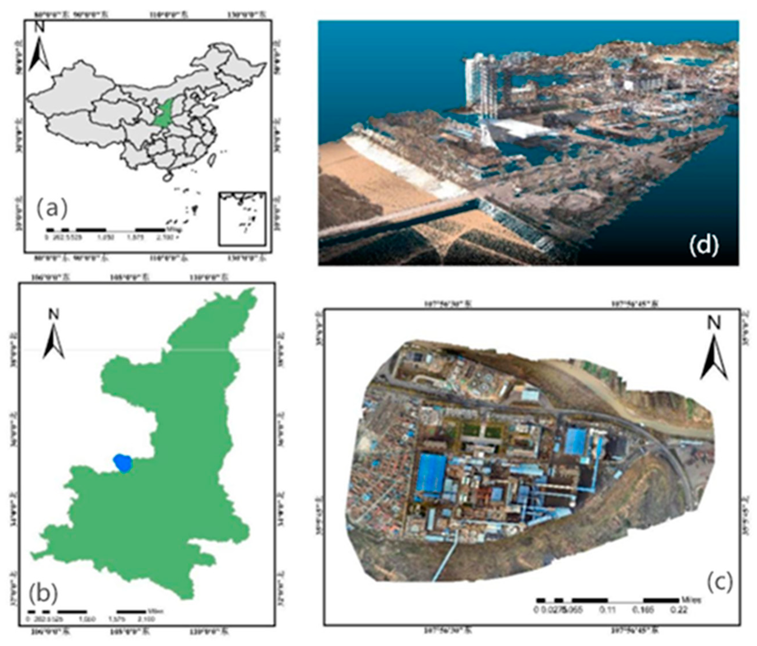
Figure 3.
Flowchart of the test method: (a)Technical Flow Chart; (b)Flowchart of Combined Filtering Algorithm.
Figure 3.
Flowchart of the test method: (a)Technical Flow Chart; (b)Flowchart of Combined Filtering Algorithm.
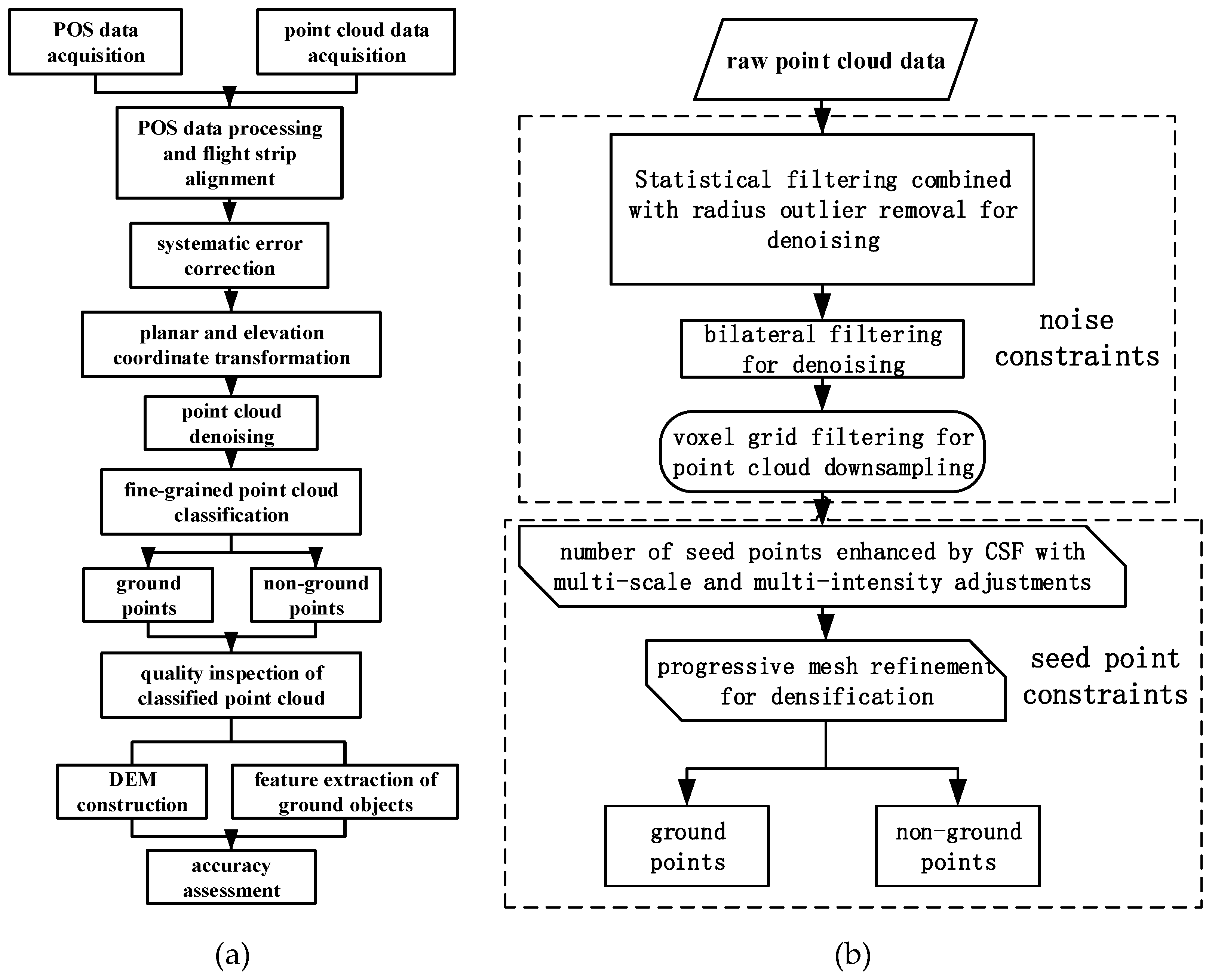
Figure 5.
At each density level, the point cloud of flat terrain generates elevation frequency histogram:(a) 90% Sampling rate ; (b) 70% Sampling rate; (c) 50% Sampling rate;(d) 30% Sampling rate.
Figure 5.
At each density level, the point cloud of flat terrain generates elevation frequency histogram:(a) 90% Sampling rate ; (b) 70% Sampling rate; (c) 50% Sampling rate;(d) 30% Sampling rate.
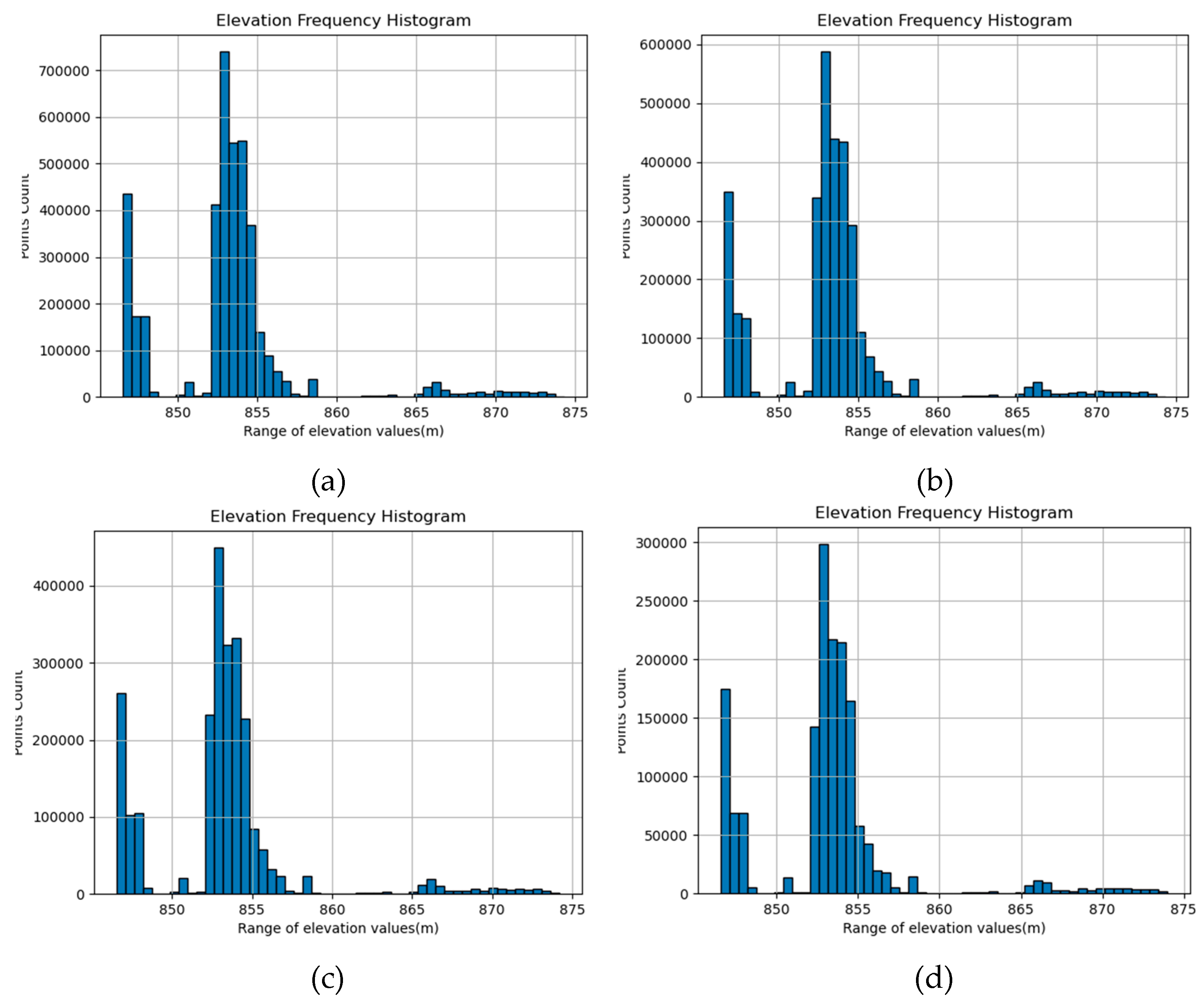
Figure 6.
The elevation frequency histogram is generated by the point cloud of gully topography at each density level: (a) 90% Sampling rate; (b) 70% Sampling rate;(c) 50% Sampling rate ; (d) 30% Sampling rate.
Figure 6.
The elevation frequency histogram is generated by the point cloud of gully topography at each density level: (a) 90% Sampling rate; (b) 70% Sampling rate;(c) 50% Sampling rate ; (d) 30% Sampling rate.
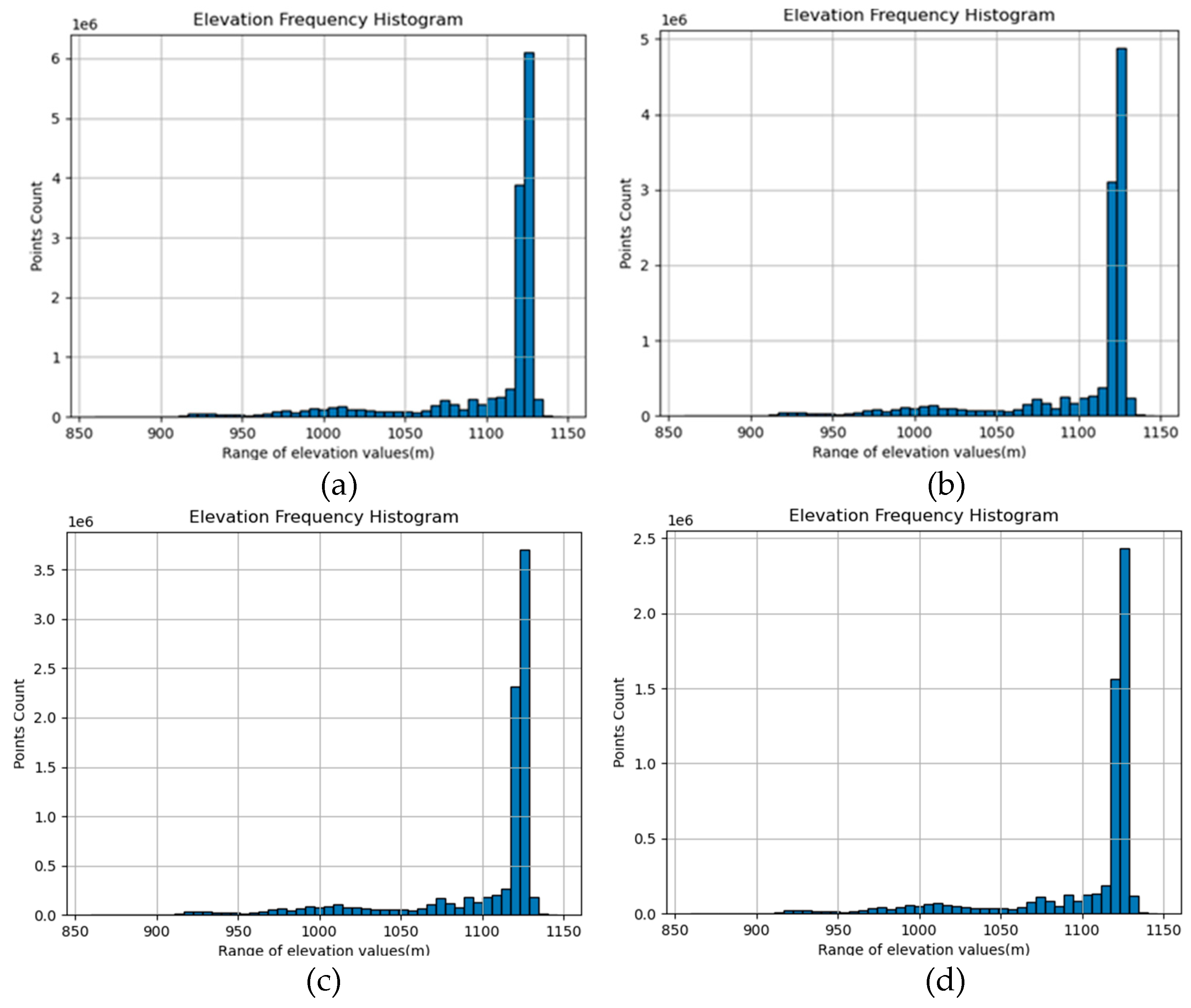
Figure 7.
Mountain shadow map formed by interpolation on flat terrain at 90% density:(a) IDW; (b) OK;(c) RBF.
Figure 7.
Mountain shadow map formed by interpolation on flat terrain at 90% density:(a) IDW; (b) OK;(c) RBF.
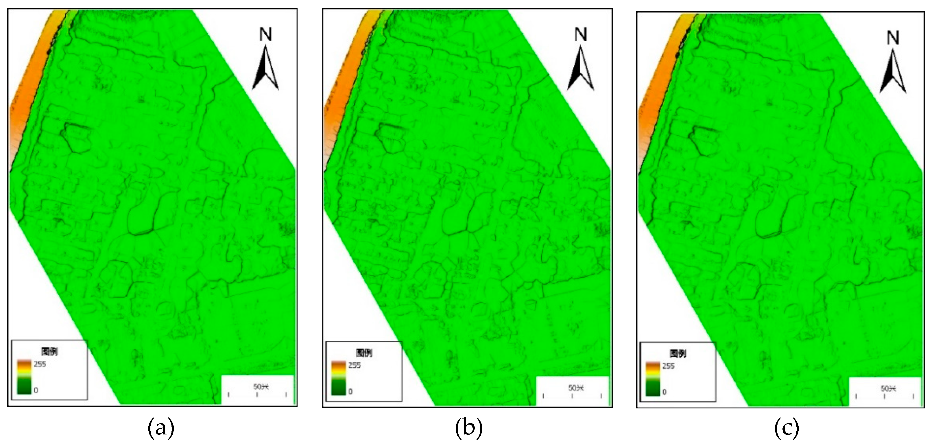
Figure 8.
Mountain shadow map formed by interpolation on flat terrain at 70% density:(a) IDW; (b) OK;(c) RBF.
Figure 8.
Mountain shadow map formed by interpolation on flat terrain at 70% density:(a) IDW; (b) OK;(c) RBF.
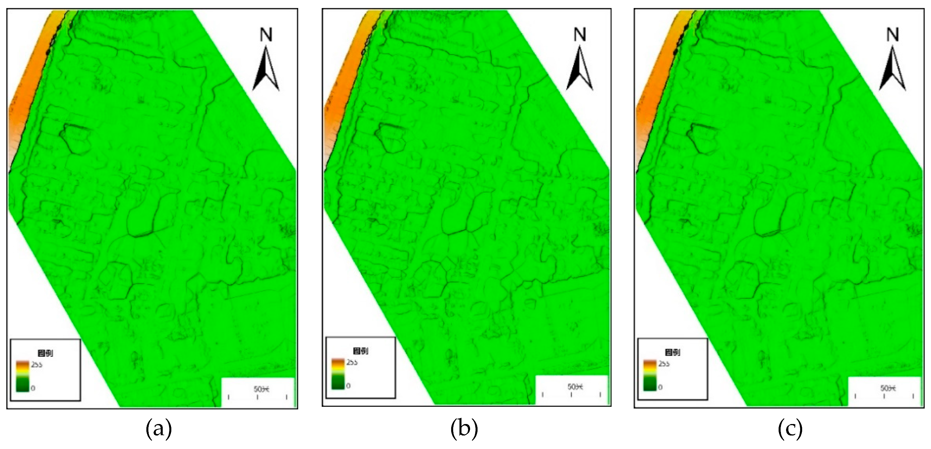
Figure 9.
Mountain shadow map formed by interpolation on flat terrain at 50% density:(a) IDW; (b) OK;(c) RBF.
Figure 9.
Mountain shadow map formed by interpolation on flat terrain at 50% density:(a) IDW; (b) OK;(c) RBF.
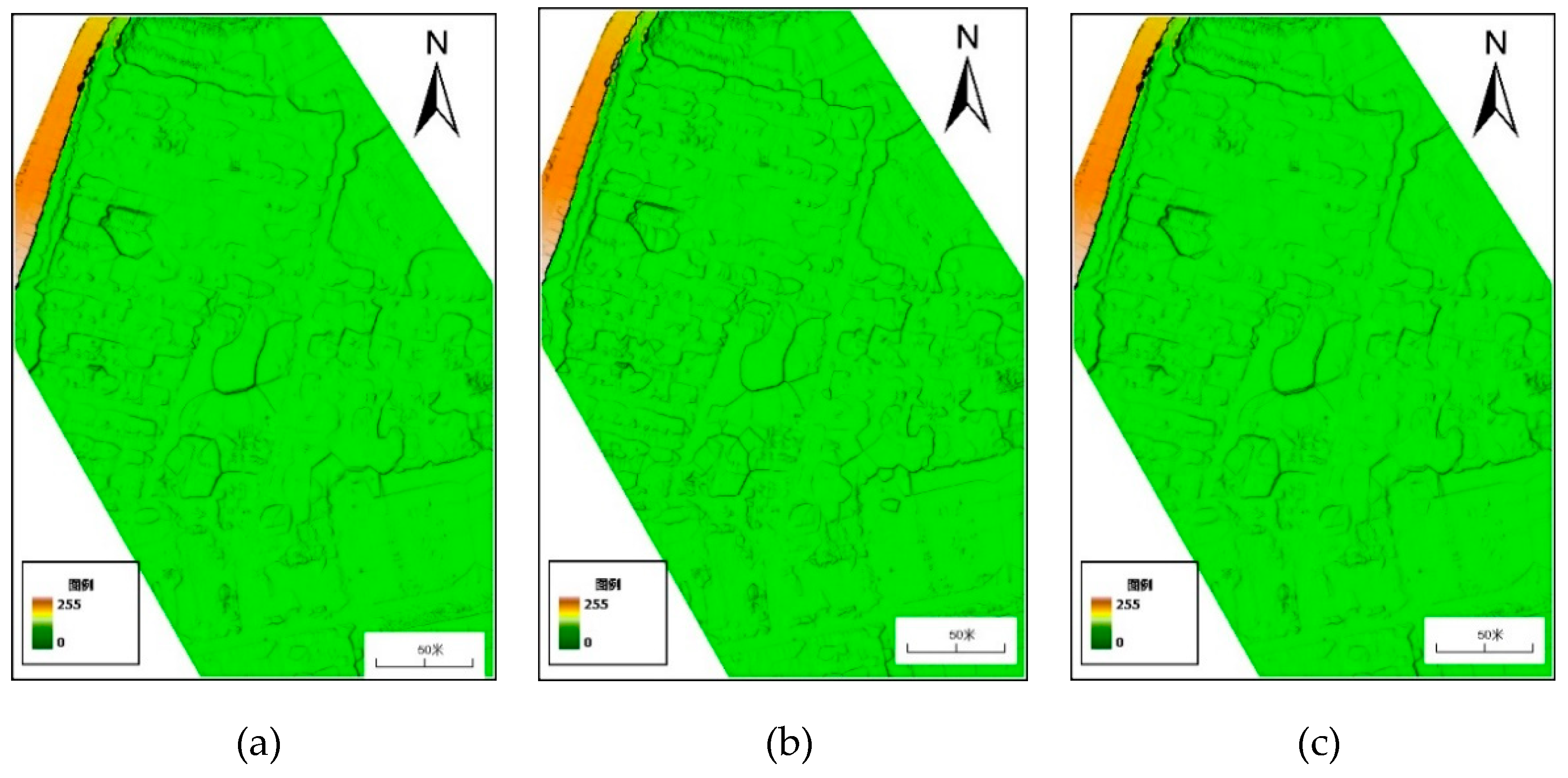
Figure 10.
Mountain shadow map formed by interpolation on flat terrain at 30% density:(a) IDW; (b) OK;(c) RBF.
Figure 10.
Mountain shadow map formed by interpolation on flat terrain at 30% density:(a) IDW; (b) OK;(c) RBF.
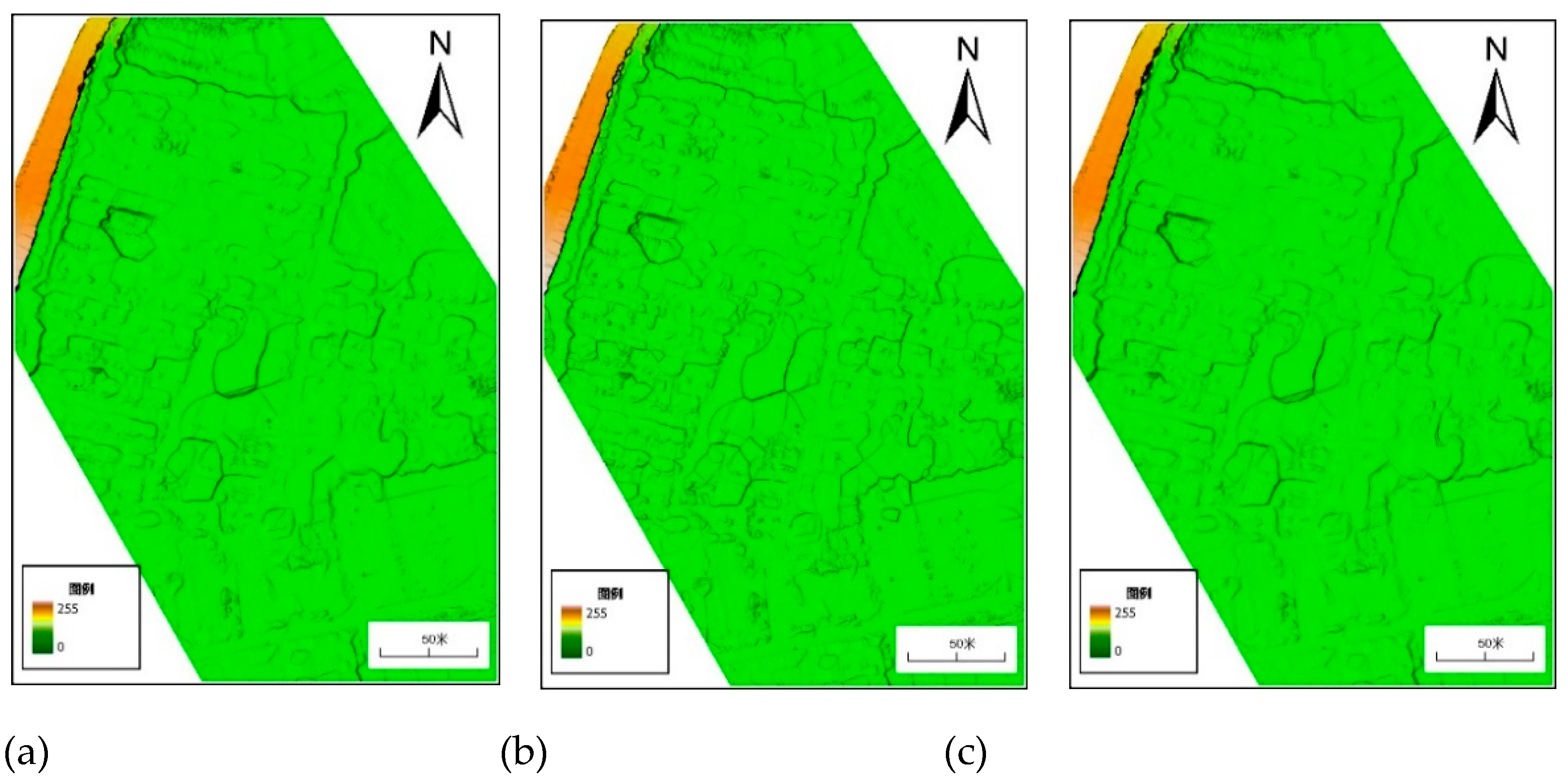
Figure 11.
Mountain shadow map formed by interpolation of gully terrain at 90% density:(a) IDW; (b) OK;(c) RBF.
Figure 11.
Mountain shadow map formed by interpolation of gully terrain at 90% density:(a) IDW; (b) OK;(c) RBF.
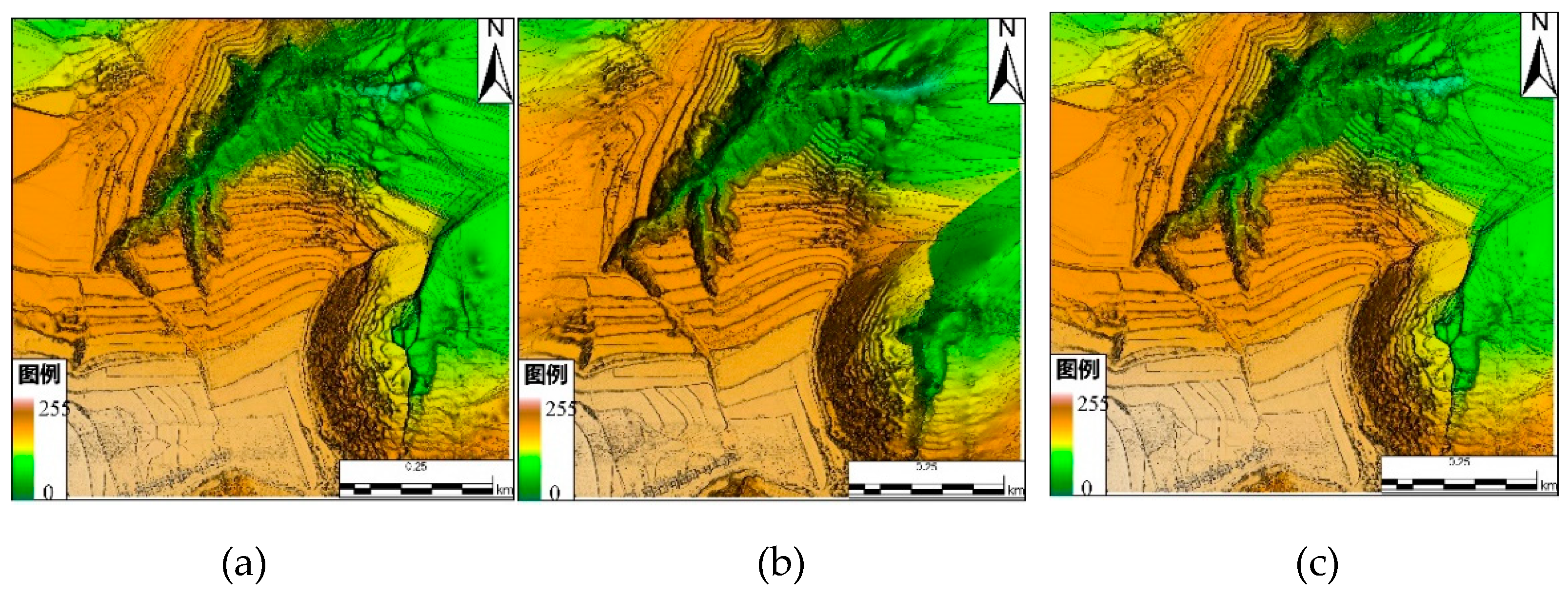
Figure 12.
Mountain shadow map formed by interpolation of gully terrain at 70% density:(a) IDW; (b) OK;(c) RBF.
Figure 12.
Mountain shadow map formed by interpolation of gully terrain at 70% density:(a) IDW; (b) OK;(c) RBF.
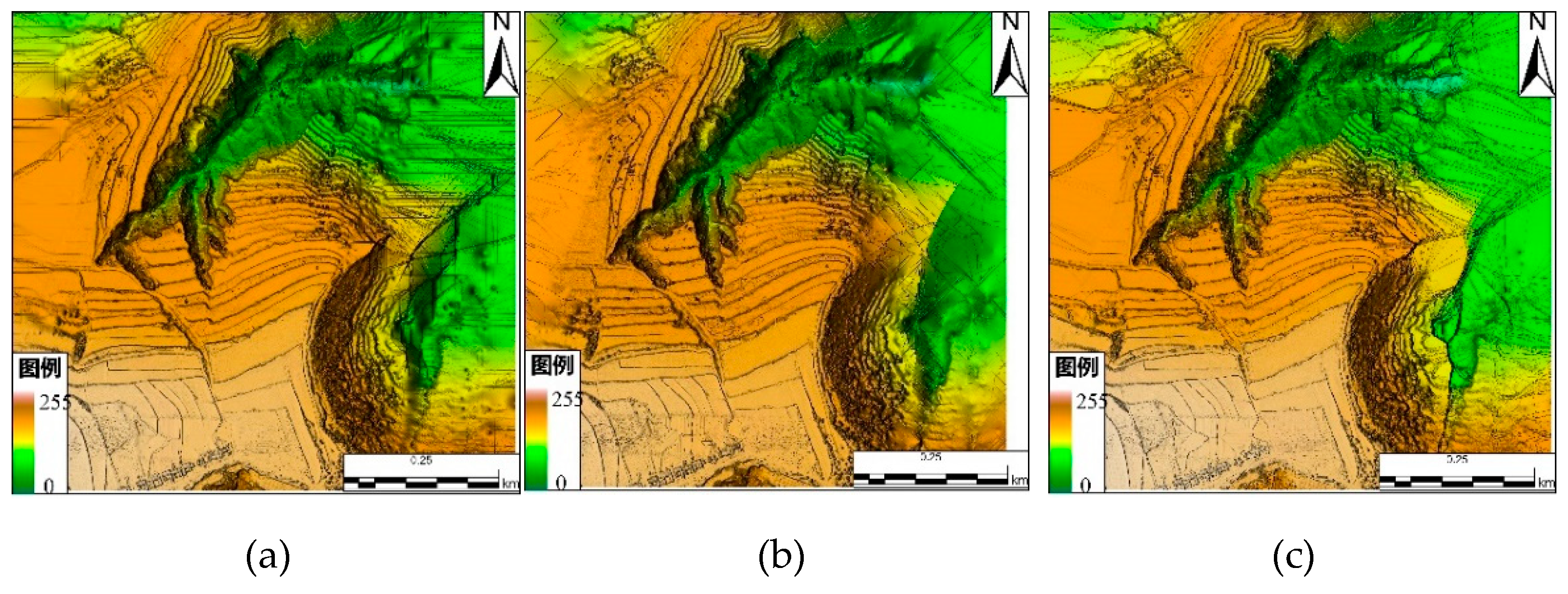
Figure 13.
Mountain shadow map formed by interpolation of gully terrain at 50% density:(a) IDW; (b) OK;(c) RBF.
Figure 13.
Mountain shadow map formed by interpolation of gully terrain at 50% density:(a) IDW; (b) OK;(c) RBF.
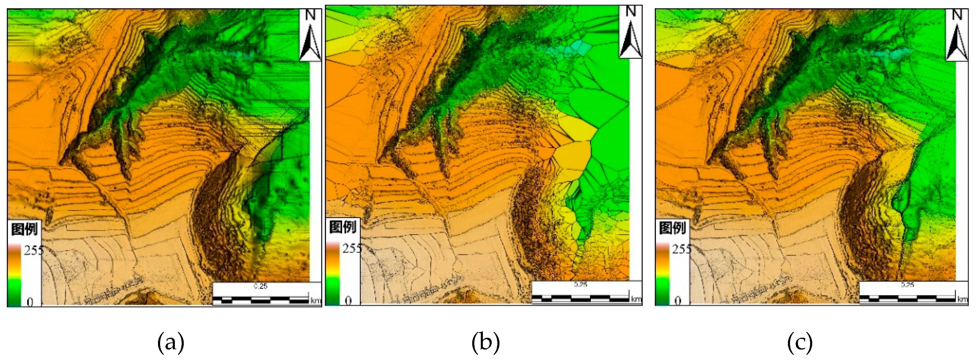
Figure 14.
Mountain shadow map formed by interpolation of gully terrain at 30% density:(a) IDW; (b) OK;(c) RBF.
Figure 14.
Mountain shadow map formed by interpolation of gully terrain at 30% density:(a) IDW; (b) OK;(c) RBF.
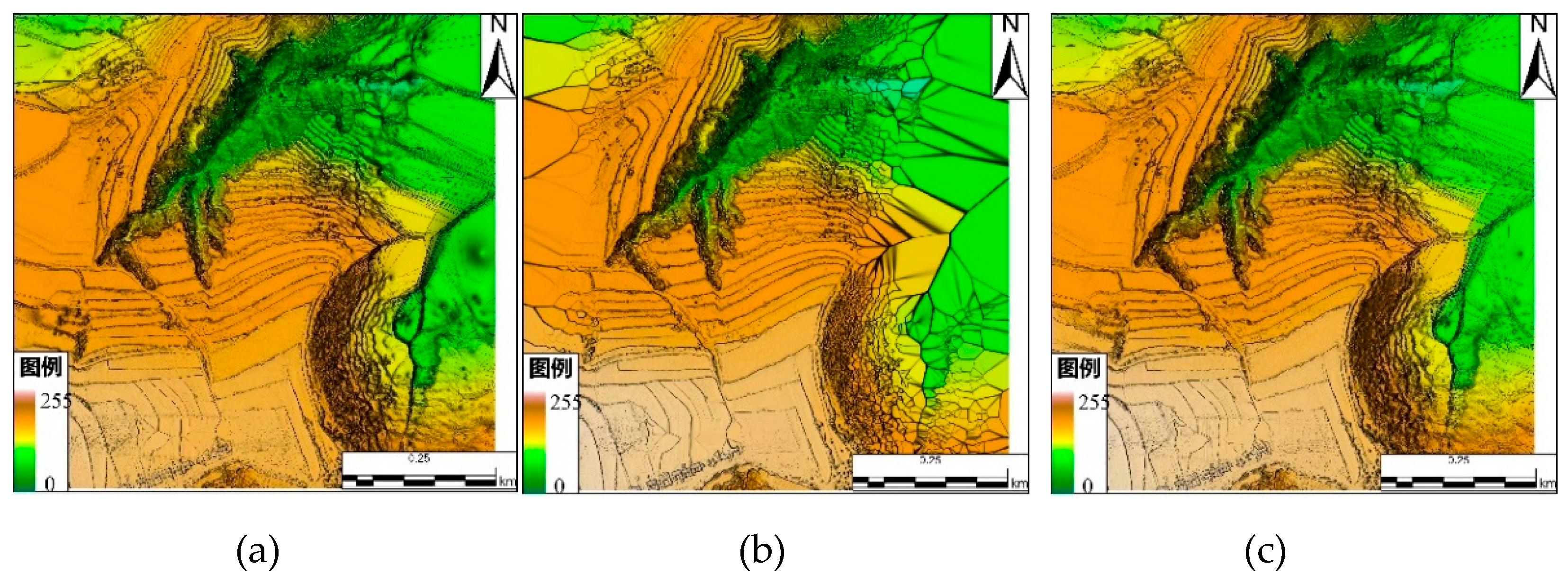
Figure 15.
Relationship between DEM error generated by each algorithm and point cloud density.
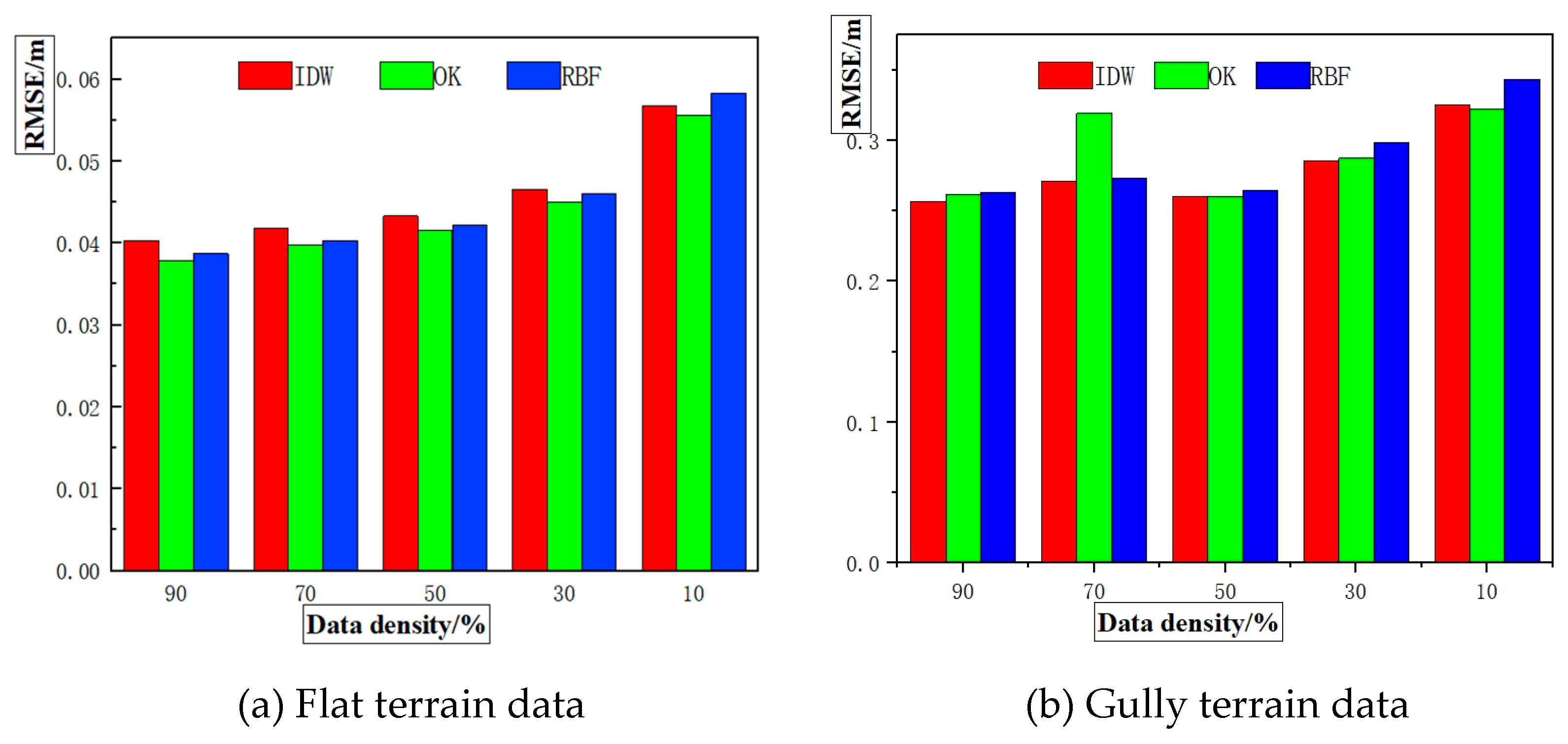
Table 1.
Original point cloud data.
| Test Area | Density/(Points/m2) | Number of Laser Point Clouds/One | Elevation Range/m |
|---|---|---|---|
| Flat terrain | 350 | 14352663 | 850.49~901.79 |
| Gully relief | 420 | 21347990 | 954.79~1139.86 |
Table 4.
RMSE of DEM obtained by various algorithms.
| Density/% | RMSE/m | |||||
|---|---|---|---|---|---|---|
| IDW | OK | RBF | ||||
| Test area | flat | gully | flat | gully | flat | gully |
| 90 | 0.0403 | 0.2565 | 0.0379 | 0.2619 | 0.0387 | 0.2629 |
| 70 | 0.0418 | 0.2708 | 0.0398 | 0.3192 | 0.0403 | 0.2731 |
| 50 | 0.0422 | 0.2599 | 0.0416 | 0.2598 | 0.0433 | 0.2648 |
| 30 | 0.0466 | 0.2857 | 0.0450 | 0.2874 | 0.0460 | 0.2985 |
| 10 | 0.0568 | 0.3255 | 0.0556 | 0.3220 | 0.0583 | 0.3435 |
Disclaimer/Publisher’s Note: The statements, opinions and data contained in all publications are solely those of the individual author(s) and contributor(s) and not of MDPI and/or the editor(s). MDPI and/or the editor(s) disclaim responsibility for any injury to people or property resulting from any ideas, methods, instructions or products referred to in the content. |
© 2024 by the authors. Licensee MDPI, Basel, Switzerland. This article is an open access article distributed under the terms and conditions of the Creative Commons Attribution (CC BY) license (http://creativecommons.org/licenses/by/4.0/).
Copyright: This open access article is published under a Creative Commons CC BY 4.0 license, which permit the free download, distribution, and reuse, provided that the author and preprint are cited in any reuse.


