Monetary Policy Under Global and Spillover Uncertainty Shocks: What Do the Bayesian Time-Varying Coefficient Var, Local Projections, and Vecm Tell Us in Tunisia?

1. Introduction

The optimal design of monetary policy is a challenging task for central banks who always seek the ultimate objective of price stabilization (Sliman, 2008, Sghaier and Abida, 2013; Hammami, 2016; Turki and Lajnaf, 2024). Tunisia, like other countries, has known evolving monetary policy conduct stages following special events such as the global financial crisis. The most dramatic episode is the one following the transition period, known as the 2011 revolution (Guizani, 2015). The economic situation has been marked by a worsening of the current account and budget deficits, an increase in the unemployment rate, and an economic recession with a fall in GDP (Chtourou and Hammami, 2014). Price stability remains the main objective of the monetary policy but there is no explicit nominal anchor. The Central Bank of Tunisia (CBT) has taken steps toward a transition to inflation targeting without real success (Zouhair and Younes, 2009; Kadria and Ben Aissa, 2014; End et al., 2020; Trabelsi and Ben Khaled, 2023). Following the fall of the Ben Ali regime, CBT applied an accommodative monetary policy. In 2012, monetary policy tightened with an increase in key interest rates. In addition to the depreciation of the dinar, inflation was fueled by the rise in oil prices and wage increases. There was also a mismatch between supply and demand for goods and services. Banks granted credit to potentially insolvent customers, increasing non-performing loans (Charfi, 2016). The situation seems not to be the best with the arrival of COVID-19, plunging the economy back into recession and further uncertainty (Mansour and Ben Salem, 2020). The spread of the epidemic and the need for short-, medium- and long-term visibility suggest that viewers feared the worst, either a surge in expansion versus negative growth or a circumstance of Stagflation with devastating financial and social consequences. Pandemics, crises, and political instability are perturbing events that generate global uncertainty (Gupta and Jooste, 2018). In this regard, Cascaldi-Garcia et al. (2021) show that there has been a growing emphasis among scholars, decision-makers, and economic agents on the impact of risk and uncertainty on financial markets and economic expectations.

It is widely admitted that uncertainty shocks can drive aggregate fluctuations and explain monetary policy transmission mechanisms in modern business cycle research (Bloom, 2009; Basu and Bundick, 2017; Fernández-Villaverde and Guerrón-Quintana, 2020; Cho et al., 2021; Bianchi et al., 2023) but the related measures are expansive and categorized (Caldara et al., 2016; Kozeniauskas and Veldkamp, 2018; Cascaldi-Garcia et al., 2021). We focus on global shocks related to economic, financial, pandemic, and oil price uncertainties. We depart from the view that global and spillover shocks have a larger impact on monetary policy and economic output than local shocks (e.g., Bloom, 2009; Colombo, 2013; Carrière-Swallow and Céspedes, 2013; Handley, 2014; Handley and Limao, 2015; Jones and Olson, 2015; Carriero et al., 2015; Cheng, 2017; Azad, 2022). Using a novel Bayesian VAR with time-varying coefficients, we disentangle the response of the Tunisian monetary policy to multiple uncertainty shocks. As Geraci and Gnabo (2018) put it, we create a statistical framework based on the market that models the dynamic nature of connections between financial institutions using Bayesian estimation of time-varying parameter vector autoregressions (TVP-VAR). Unlike the classical approach, which favors abrupt, frequently unjustified changes in interconnectedness, the framework permits connections to evolve gradually over time. The approach enables us to reconstruct a dynamic network of directed spillover and global effects. As Fischer et al. (2023) claimed, the core of our estimation technique is the specification of appropriate shrinkage priors that allow us to reduce coefficients toward zero concerning effect modifiers that are not important. Since the TVP-VARs depend linearly on the action modifiers, these priorities allow combinations of multiple motion laws and can endogenously determine the correct motion law for the parameters. The model examines factors affecting parameter variation over time. Another flexible solution is to rely on Local Projections (LPs). Jordà and Taylor (2024, p.1) stated that “Local projections (or LPs) are a sequence of regressions where the outcome, dated at increasingly distant horizons, is regressed on the intervention (directly, if randomly assigned; or perhaps instrumented, if not), conditional on a set of controls that include lags of both the outcome and the intervention, as well as other exogenous or predetermined variables”. Our results indicate that different uncertainty measures explain a statistically significant portion of macroeconomic fluctuations, causing a decline in industrial production and a rise in both the money market rate and consumer price index. Our approach is inspired by Dery and Serletis (2021a, 2021b). We differ from their contributions in three main aspects: We analyze a wide range of uncertainty shocks, including real and monetary policy shocks, surpassing previous literature that often focused on only one aspect of local uncertainty. We assess the forecasting ability of uncertainty shock measures for real economic activity and monetary policy, identifying which measure has predictive power. We use Toda and Yamamoto's (1995) Granger causality test to evaluate the relationship between uncertainty measures and industrial production, the consumer price index, monetary aggregates, the real effective exchange rate, and the money market rate. Third, while risk can be a potential informative tool in explaining Tunisian monetary policy, we discard the related measures as this goes beyond the scope of the paper and is left for future investigation.

Our paper also takes an intriguing step to highlight specific mechanisms that drive the impact of uncertainty on the real economy and prices by calling the irreversibility theory. This theory suggests that firms often delay investment and hiring during uncertain times. There are two main ways in which uncertainty affects firms. First, the real option, given the irreversibility of the investment, shows the importance of waiting and being flexible when making investment decisions in response to uncertainty (Bernanke, 1983; Bertola and Caballero, 1994; Caballero and Pindyck, 1996). Second, during periods of uncertainty, higher risk premiums increase the amount of money to compensate borrowers for losses due to increased uncertainty (Bhatia and Pratap, 2024). Therefore, when faced with high uncertainty, agents adopt more strategic plans, which leads to reduced long-term investments. In our context, this implies investigating the effectiveness of the money market rate as a monetary policy instrument of CBT during high uncertainty times in a VECM where the interest rate interacts with uncertainty variables. If the interest rate does not significantly impact the relationship between uncertainty indices and the real economy and prices, it indicates that the interest rate is a less influential tool, leading economic agents to adopt a “wait and see” (precautionary) approach. This investigation enhances the uniqueness of our research. Our contribution seeks to address a significant research gap in the Tunisian context.

The layout of the paper is given as follows. In Section 2, we provide theoretical and empirical arguments about transmitting channels of uncertainty shocks to emerging countries, including Tunisia. Section 3 describes the process of data collection and empirical strategy. We expose and discuss our findings in Section 4. Section 5 concludes with policy implications.

2. Literature Review

2.1. Monetary Policy and Global Uncertainty: Spillover Effects in Emerging Economies

The discourse on the impact of global uncertainty on monetary policy is grounded in several theoretical frameworks. Frankel (2010) delineated the distinguishing characteristics of developing countries compared to industrialized nations, noting their heightened susceptibility to supply shocks and diminished credibility regarding price stability. In conjunction with this perspective, Castelnuovo (2023) examined the nonlinear effects of uncertainty shocks and their pivotal role in driving business cycles. Furthermore, the review by Fernández-Villaverde and Guerrón-Quintana (2020) scrutinized various theoretical frameworks to elucidate the transmission channels of uncertainty shocks within Dynamic Stochastic General Equilibrium (DSGE) models. This analysis highlights the critical issues related to communication and credibility that significantly influence monetary policy decisions.

Survey studies conducted by Bloom (2014), Carriero et al. (2021), and Castelnuovo (2023) have underlined the critical need for further exploration of the macroeconomic effects of spillover and global uncertainty. A common feature emerges: uncertainty plays a significant role as a driver of the business cycle, necessitating a comprehensive analysis of its nonlinear effects, particularly on financial frictions and policy interventions (Lakdawala et al., 2021).

A substantial body of empirical research has sought to elucidate the effects of global policy uncertainty on emerging markets. Azad and Serletis (2022a) showed that US monetary policy uncertainty adversely affects the macroeconomic and financial fundamentals of emerging economies. Complementing these findings, Prabheesh et al. (2021) identified that uncertainty arising from the COVID-19 pandemic attenuated the effectiveness of monetary policy transmission to inflation. However, some economies succeeded in stabilizing credit and output despite heightened uncertainty. The work of Lastauskas and Nguyen (2024) further elucidated how US monetary policy shocks instigated co-movements in international financial variables, thereby contributing to a global financial cycle that interconnected diverse economic landscapes. 

This interconnectedness becomes particularly salient when examining US monetary policy uncertainty and its substantial repercussions for emerging markets (Bhattarai et al., 2017; Olanipekun and Olasehinde-Williams, 2022). Aor et al. (2021) found that shocks stemming from US monetary policy uncertainty had temporary negative effects on real equity prices across both advanced and emerging economies. Additionally, Park and Kim (2021) highlighted that the US monetary policy in the post-quantitative easing era adversely affected the KRW/USD exchange rate in South Korea, while exerting minimal influence on domestic macroeconomic variables such as output and consumer prices. Anaya et al. (2017) observed that emerging markets typically responded to unconventional US monetary policy shocks by easing their monetary stances, with these shocks being transmitted through international capital flows. Echoing this sentiment, Bhattarai et al. (2020) illustrated how US uncertainty shocks resulted in reductions in output and consumer prices in emerging markets, thus complicating monetary policy responses. This evidence points to a negative effect of US monetary tightening brought on by a more hawkish policy stance (Ahmed et al., 2021; De Leo et al., 2022). As a result, trade-offs are likely to occur when inflation expectations are firmly anchored in emerging economies.

The implications of world uncertainty for monetary policy have also been explored across various contexts (see Canh et al., 2020). Gu et al. (2021) investigated the effects of global economic policy uncertainty, revealing its significant empirical impact on stock volatility in nine emerging economies. This influence extended to Latin America, where Aytaç and Saraç (2022) reported that economic policy uncertainty led to rising inflation and interest rates in several countries. The adverse long-term effects of economic policy uncertainty on economic expectations are further depicted by Al-Thaqeb and Algharabali (2019), Al-Thaqeb et al. (2022), and Ben Cheikh et al. (2023). Additionally, Montes and Marcelino (2023) demonstrated that heightened economic policy uncertainty amplified disagreement among economic agents regarding fiscal and monetary policy, thereby complicating the navigation of uncertainty in policymaking (see Athari et al., 2022; Anderl and Caporale, 2023; Pagliacci, 2023; Sengupta et al., 2024).

The interconnected nature of global financial systems is further reinforced by the influence of US financial stress on the monetary policies of emerging markets. Financial stress pertains to interruptions to normal economic activities and the ongoing volatility observed in financial markets (Das et al., 2018; Choi and Shim, 2019; Polat, 2020; Jana et al., 2022; Gosh et al., 2024). Tng and Kwek (2015) noted that increased financial stress resulted in tighter credit conditions and diminished economic activity across ASEAN countries, highlighting the necessity for targeted policy measures to restore financial stability. This assertion was corroborated by Ghosh et al. (2024), who elucidated how financial stress reflects disruptions to regular economic activities, particularly during volatile regimes such as the COVID-19 pandemic. Moreover, Fink and Shüler (2015) and Niepmann et al. (2021) emphasized that US systemic financial stress shocks significantly drove economic dynamics and fluctuations in emerging markets, reinforcing the interconnectedness that shapes monetary policy responses. The result complements previous studies such as Lown and Morgan (2006), Helbling et al. (2011), Baxa et al., 2013; Kalemli-Ozcan et al. (2013), Hristov et al. (2012), Gilchrist et al. (2014), and Schüler (2014). Moreover, Tobal and Menna (2020) contended that the interplay between monetary policy and financial stress in emerging markets is inherently complex. The authors advocated for the development of models capable of capturing financial crises as endogenous phenomena, stemming from the accumulation of financial imbalances. Such insights are pivotal for enhancing our understanding of the broader economic implications of uncertainty in the contemporary global landscape.

In this context, oil price uncertainty has emerged as a critical factor with significant implications for monetary policy (Azad and Serletis, 2022b). Ghosh et al. (2021) illustrated how oil prices, in conjunction with financial volatility and economic policy uncertainty, influenced inflation expectations in India. Chowdhury (2024) argued that oil price uncertainty significantly contributed to inflation, particularly in developing countries, while highlighting the importance of differentiating between nominal and real uncertainty to better understand output growth. Additionally, Abiad and Qureshi (2021) found that oil price uncertainty negatively affects macroeconomic activity, particularly under zero lower-bound constraints on monetary policy.  Su et al. (2021) argued that oil price shocks positively affect economic policy uncertainty when oil markets experience supply shocks, a result supported by Shahbaz et al. (2023). Evidence about the interaction of economic policy uncertainty and oil price is found in Sun et al. (2020), Chen et al. (2020), and Lin and Bai (2021).

The literature review highlights the complex relationship between global uncertainty, spillover effects, and monetary policy in emerging markets. Insights from theoretical frameworks and empirical studies highlight the challenges policymakers encounter in managing uncertainty in the interconnected global economy (Baharumshah et al., 2016).

2.2. Tunisia's Monetary Policy in the Face of Global and Domestic Shocks

The spillover effects of global uncertainty shocks on Tunisia's monetary policy were the focus of extensive empirical research, revealing the complex challenges faced by the CBT in stabilizing the economy. Trabelsi and Ben Khaled (2023) demonstrated that global uncertainties, as captured by the World Uncertainty Index, significantly contributed to inflationary pressures in Tunisia, hindering the country's transition to an inflation-targeting regime. They argued that adopting a flexible exchange rate and increasing monetary policy transparency was crucial for overcoming these barriers. In a complementary study, Turki and Gabsi (2023) found that global uncertainty adversely affects aggregate demand and economic activity, rendering conventional monetary tools insufficient during periods of heightened risk. The domestic dimension of uncertainty was also critical. Belhoula (2024) showed that local economic policy uncertainty resulted in negative shifts in growth, consumption, and industrial output, underscoring the need for consistent and coherent policy frameworks. Similarly, Jallouli and Yalouli (2022) highlighted the limitations of monetary policy when subjected to uncertainty shocks from external crises, including pandemics, terrorism, and political unrest. Their findings suggested that Tunisia's monetary policy needs refinement to withstand such volatility. Moving toward a more structured approach, Guizani and Wierzbowska (2022) reported a shift toward rule-based monetary frameworks in Tunisia and Morocco during the post-Arab Spring period, a shift further supported by Mimoun et al. (2024), who advocated for a rule-based inflation-targeting regime. They emphasized that supply-side policies were necessary to promote growth and correct fiscal imbalances. In a broader African context, Moyo and Phiri (2024) identified that countries more responsive to U.S. monetary policy shocks tended to experience lower inflation, suggesting that Tunisia could have benefited from improved coordination with global monetary authorities. On the financial front, Guenichi and Nejib (2022) explored the negative impacts of pandemic-related uncertainty on Tunisia’s stock market, noting the market's resilience in late 2021. Lastly, Neaime and Gaysset (2022) underscored the vulnerability of Tunisia and other MENA countries to external oil price shocks, recommending non-conventional monetary tools to mitigate these risks. Trabelsi (2024) further emphasized the role of uncertainty in driving Tunisia’s macroeconomic fluctuations, reinforcing the importance of robust policy responses.

3. Materials & Methods

3.1. Data Collection

We collect macroeconomic and financial data from various databases (see Table 1). After a cleaning process, we get a balanced sample of 90 observations running from 1997q1 to 2019q2, except for the variable (LOG(USFSI)) whose values end in 2016q4. The variables of interest comprise the Global Economic Policy Uncertainty Index which is a GDP-weighted average of 21 national economic policy uncertainty indices. There are two versions of the Index - one based on current-price GDP measures (LOG(GEPUC)), and one based on PPP-adjusted GDP (LOG(GEPUP)). To assess economic uncertainty linked to policy, Baker et al. (2016) developed an index based on three key components. The first and most adaptable component measures the frequency of policy-related economic uncertainty in newspaper articles. The World Uncertainty Index (LOG(WUITUN1)) is constructed by Ahir et al. (2022). They created quarterly indices of economic uncertainty for 143 countries starting in 1996, utilizing the frequency of the term "uncertainty" (and its variations) in the Economist Intelligence Unit (EIU) country reports. These reports cover significant political and economic events in each nation, as well as analysis and forecasts of political, policy, and economic conditions. We select the index related to the Tunisian context. We also use the US Monetary Policy Uncertainty Index (LOG(USMPUI)) from Baker et al. (2016). The authors identified newspaper articles that meet specific E, P, U, and M criteria. This involves flagging articles that contain at least one term from each of the following categories:

• ⁻ E: economic, economy
• ⁻ P: congress, legislation, white house, regulation, federal reserve, deficit
• ⁻ U: uncertain, uncertainty
• ⁻ M: Federal Reserve, the Fed, money supply, open market operations, quantitative easing, monetary policy, fed funds rate, overnight lending rate, Bernanke, Volker, Greenspan, central bank, interest rates, fed chairman, fed chair, lender of last resort, discount window, European Central Bank, ECB, Bank of England, Bank of Japan, BOJ, Bank of China, Bundesbank, Bank of France, Bank of Italy.

The final indices are created using scaled frequency counts of newspaper articles that mention monetary policy uncertainty. The definition of "monetary policy uncertainty" differs for each MPU index. "Scaling" is applied to account for variations in the total number of articles across different newspapers and over time.

The US Financial Stress Indicator (LOG(USFSI)) is developed by Püttmann (2018) using article titles from five major US newspapers: the Boston Globe, Chicago Tribune, Los Angeles Times, Wall Street Journal, and Washington Post. Püttmann (2018) follows a three-step process, beginning by defining eleven topics related to financial markets, which are identified through 120 specific keywords. In the second step, the sentiment of these titles is assessed using four sentiment dictionaries, determining whether each title has a net negative connotation. Finally, Püttmann (2018) standardizes the monthly financial sentiment index to a mean of 100 with a unit standard deviation, averaging across various newspaper-dictionary combinations to create his quarterly FSI.  All variables are transformed using the natural logarithm. Finally, we consider the shocks from the Oil Price Uncertainty Index (LOG(OILUI)) according to Abiad and Qureshi (2023). The method is analogous to measuring economic policy uncertainty. The analysis focuses on a collection of English-language articles containing a minimum of 100 words from 50 newspapers globally. The selection process excludes non-standard news items, such as sports articles, editorials, abstracts, advertisements, sponsored content, blogs, opinion pieces, country profiles, transcripts, press releases, and similar content.

Table 1. Summary of variables.

Variable	Acronym	Definition	Source
Economic activity	LOG(IPIT)	Industrial production index, all items	National Institute of Statistics (NIS)
Inflation	LOG(CPI)	Consumer price index, all items	NIS
Monetary aggregate	LOG(M2TND)	Money supply converted from monthly data	Central Bank of Tunisia (CBT)
Money Market rate	TMM	Money market rate converted from monthly data	CBT
Real Effective Exchange rate	LOG(TCER)	Real effective exchange rate, convertedfrom monthly data. It is the Tunisian dinar against a basket of foreign currencies divided by price deflator. If TCER increases, it indicates an appreciation of local money. The latter has strengthened against foreign currencies.	International Financial Statistics (IFS)
Global Economic Uncertainty	LOG(GEPUC)	Global Economic Policy Uncertainty index - based on current-price GDP developed by Baker et al. (2016), convertedfrom monthly data	https://www.policyuncertainty.com/
Global Economic Uncertainty	LOG(GEPUP)	Global Economic Policy Uncertainty Index - based on PPP-adjusted GDP developed by Baker et al. (2016), convertedfrom monthly data	https://www.policyuncertainty.com/
World Uncertainty	LOG(WUITUN1)	World Uncertainty Index related to Tunisia developed by Ahir et al. (2022)	https://www.worlduncertaintyindex.com/
Monetary Policy Uncertainty	LOG(USMPUI)	US Monetary Policy Uncertainty convertedfrom monthly data	https://www.policyuncertainty.com/
Financial Stress	LOG(USFSI)	US Financial Stress Index	https://www.policyuncertainty.com/
Oil uncertainty	LOG(OILUI)	Oil Price Uncertainty Index, convertedfrom monthly data	https://www.policyuncertainty.com/

Table 1. Summary of variables.

Variable	Acronym	Definition	Source
Economic activity	LOG(IPIT)	Industrial production index, all items	National Institute of Statistics (NIS)
Inflation	LOG(CPI)	Consumer price index, all items	NIS
Monetary aggregate	LOG(M2TND)	Money supply converted from monthly data	Central Bank of Tunisia (CBT)
Money Market rate	TMM	Money market rate converted from monthly data	CBT
Real Effective Exchange rate	LOG(TCER)	Real effective exchange rate, convertedfrom monthly data. It is the Tunisian dinar against a basket of foreign currencies divided by price deflator. If TCER increases, it indicates an appreciation of local money. The latter has strengthened against foreign currencies.	International Financial Statistics (IFS)
Global Economic Uncertainty	LOG(GEPUC)	Global Economic Policy Uncertainty index - based on current-price GDP developed by Baker et al. (2016), convertedfrom monthly data	https://www.policyuncertainty.com/
Global Economic Uncertainty	LOG(GEPUP)	Global Economic Policy Uncertainty Index - based on PPP-adjusted GDP developed by Baker et al. (2016), convertedfrom monthly data	https://www.policyuncertainty.com/
World Uncertainty	LOG(WUITUN1)	World Uncertainty Index related to Tunisia developed by Ahir et al. (2022)	https://www.worlduncertaintyindex.com/
Monetary Policy Uncertainty	LOG(USMPUI)	US Monetary Policy Uncertainty convertedfrom monthly data	https://www.policyuncertainty.com/
Financial Stress	LOG(USFSI)	US Financial Stress Index	https://www.policyuncertainty.com/
Oil uncertainty	LOG(OILUI)	Oil Price Uncertainty Index, convertedfrom monthly data	https://www.policyuncertainty.com/

Summary statistics are available in Table 2. The mean values of the variable range from 0.17 (LOG(WUITUN1)) to 10.25 (LOG(M2TND)), with LOG(M2TND) having the highest average, indicating the importance of money supply in the dataset. Standard deviations suggest moderate variability, with TMM (money market rates) being the most volatile (0.97) and LOG(USFSI) the most stable (0.008). Skewness values are generally close to zero, indicating relatively symmetric distributions, although LOG(WUITUN1) is positively skewed (1.022). Kurtosis values vary, with most variables being close to 3, indicating a normal distribution shape, except for LOG(CPI) and LOG(M2TND), which have flatter distributions. The results of the Jarque-Bera test indicate that LOG(IPIT) and LOG(WUITUN1) are not normally distributed (p-value = 0.00396, p-value = 0.000388, respectively). Most other variables are closer to normality. Observations are consistent across variables, with a slight decrease for LOG(USFSI).

Table 2. Descriptive statistics.

Statistics	LOG(IPIT)	LOG(CPI)	LOG(M2TND)	TMM	LOG(TCER)	LOG(GEPUC)	LOG(GEPUP)	LOG(WUITUN	1)LOG(USMPUI)	LOG(USFSI)	LOG(OILUI)
Mean	4.493770	4.556945	10.24873	5.275107	4.666892	4.672641	4.670963	0.165609	4.647079	4.617030	4.538725
Median	4.521680	4.524614	10.28769	5.000000	4.638794	4.683143	4.670338	0.106669	4.645387	4.617074	4.621765
Maximum	4.628232	5.038763	11.26710	7.840000	4.893060	5.520925	5.580722	0.703028	5.495236	4.647271	5.776230
Minimum	4.241714	4.204875	9.074444	3.236670	4.298770	4.014913	4.044697	0.000000	3.770833	4.604242	2.717981
Std. Dev.	0.093333	0.234030	0.656923	0.974519	0.160428	0.381576	0.388171	0.182125	0.368397	0.008561	0.650636
Skewness	-0.855104	0.347672	-0.171137	0.486475	-0.181783	0.240665	0.326950	1.022088	-0.017403	0.676738	-0.523287
Kurtosis	3.158268	1.976452	1.756898	2.788833	2.184759	2.274641	2.340432	3.099567	2.704734	3.695873	3.056681
Jarque-Bera	11.06197	5.741832	6.234205	3.717089	2.987991	2.841840	3.234809	15.70714	0.331475	7.720455	4.119487
Probability	0.003962	0.056647	0.044285	0.155899	0.224474	0.241492	0.198413	0.000388	0.847269	0.021063	0.127487
Sum	404.4393	410.1250	922.3858	474.7596	420.0203	420.5377	420.3866	14.90482	418.2371	369.3624	408.4852
Sum Sq. Dev.	0.775282	4.874528	38.40778	84.52223	2.290610	12.95840	13.41025	2.952091	12.07878	0.005790	37.67609
Observations	90	90	90	90	90	90	90	90	90	80	90

Note: See details in Table 1 for definitions.

Table 2. Descriptive statistics.

Statistics	LOG(IPIT)	LOG(CPI)	LOG(M2TND)	TMM	LOG(TCER)	LOG(GEPUC)	LOG(GEPUP)	LOG(WUITUN	1)LOG(USMPUI)	LOG(USFSI)	LOG(OILUI)
Mean	4.493770	4.556945	10.24873	5.275107	4.666892	4.672641	4.670963	0.165609	4.647079	4.617030	4.538725
Median	4.521680	4.524614	10.28769	5.000000	4.638794	4.683143	4.670338	0.106669	4.645387	4.617074	4.621765
Maximum	4.628232	5.038763	11.26710	7.840000	4.893060	5.520925	5.580722	0.703028	5.495236	4.647271	5.776230
Minimum	4.241714	4.204875	9.074444	3.236670	4.298770	4.014913	4.044697	0.000000	3.770833	4.604242	2.717981
Std. Dev.	0.093333	0.234030	0.656923	0.974519	0.160428	0.381576	0.388171	0.182125	0.368397	0.008561	0.650636
Skewness	-0.855104	0.347672	-0.171137	0.486475	-0.181783	0.240665	0.326950	1.022088	-0.017403	0.676738	-0.523287
Kurtosis	3.158268	1.976452	1.756898	2.788833	2.184759	2.274641	2.340432	3.099567	2.704734	3.695873	3.056681
Jarque-Bera	11.06197	5.741832	6.234205	3.717089	2.987991	2.841840	3.234809	15.70714	0.331475	7.720455	4.119487
Probability	0.003962	0.056647	0.044285	0.155899	0.224474	0.241492	0.198413	0.000388	0.847269	0.021063	0.127487
Sum	404.4393	410.1250	922.3858	474.7596	420.0203	420.5377	420.3866	14.90482	418.2371	369.3624	408.4852
Sum Sq. Dev.	0.775282	4.874528	38.40778	84.52223	2.290610	12.95840	13.41025	2.952091	12.07878	0.005790	37.67609
Observations	90	90	90	90	90	90	90	90	90	80	90

Note: See details in Table 1 for definitions.

The pairwise correlation analysis reveals several key relationships among the economic and financial variables (see Table 3). Industrial production (LOG(IPIT)) shows strong positive correlations with both consumer price index (LOG(CPI), 0.79) and money supply (LOG(M2TND), 0.86), suggesting that higher industrial activity is associated with inflation and increased money supply. LOG(CPI) and LOG(M2TND) are almost perfectly correlated (0.99), reflecting a close link between inflation and monetary expansion. In contrast, money market rates (TMM) exhibit strong negative correlations with LOG(IPI) (-0.81), LOG(CPI) (-0.82), and LOG(M2TND) (-0.87), highlighting the typical inverse relationship where higher interest rates suppress industrial output and inflation.

Similarly, the real effective exchange rate (LOG(TCER)) has strong negative correlations with LOG(CPI) (-0.95) and LOG(M2TND) (-0.97), indicating that inflationary pressures and monetary expansion may reduce energy consumption. Moderate positive correlations are observed between global economic policy uncertainty (LOG(GEPUC)) and both LOG(CPI) (0.62) and LOG(M2TND) (0.61), implying that uncertainty is associated with rising inflation and monetary supply. Oil prices (LOG(OILUI)) also show a moderate positive correlation with industrial production (0.58), suggesting that higher oil prices tend to accompany economic growth.

In contrast, US monetary policy uncertainty (LOG(USMPUI)) exhibits weak and insignificant correlations with other variables. US financial stress (LOG(USFSI)), however, is negatively correlated with LOG(CPI) (-0.62) and LOG(M2TND) (-0.58), suggesting that financial stress tends to rise during periods of low inflation and money supply. Additionally, LOG(USFSI) is positively correlated with TMM (0.50), signifying higher financial stress during times of increased interest rates.

Table 3. Pairwise correlation matrix.

Covariance Analysis: Ordinary
Date: 09/30/24 Time: 14:43
Sample: 1997Q1 2016Q4
Included observations: 80
Balanced sample (listwise missing value deletion)
Correlation
Probability	LOG(IPI )	LOG(CPI)	LOG(M2TND)	TMM	LOG(TCER)	LOG(GEPUC)	LOG(GEPUP)	LOG(WUITUN1)	LOG(USMPUI)	LOG(USFSI)	LOG(OILUI)
LOG(IPI )	1.000000
	-----
LOG(CPI)	0.794720	1.000000
	0.0000	-----
LOG(M2TND)	0.864751	0.985421	1.000000
	0.0000	0.0000	-----
TMM	-0.805478	-0.815654	-0.870187	1.000000
	0.0000	0.0000	0.0000	-----
LOG(TCER)	-0.850788	-0.951899	-0.972113	0.850318	1.000000
	0.0000	0.0000	0.0000	0.0000	-----
LOG(GEPUC)	0.440426	0.620187	0.610776	-0.492474	-0.539610	1.000000
	0.0000	0.0000	0.0000	0.0000	0.0000	-----
LOG(GEPUP)	0.489974	0.667960	0.662053	-0.549543	-0.598008	0.994287	1.000000
	0.0000	0.0000	0.0000	0.0000	0.0000	0.0000	-----
LOG(WUITUN1)	0.406588	0.653235	0.644516	-0.617375	-0.628559	0.552352	0.577128	1.000000
	0.0002	0.0000	0.0000	0.0000	0.0000	0.0000	0.0000	-----
LOG(USMPUI)	-0.031563	0.107769	0.053016	0.111063	0.021264	0.359261	0.317995	0.066827	1.000000
	0.7811	0.3413	0.6405	0.3267	0.8515	0.0011	0.0040	0.5559	-----
LOG(USFSI)	-0.367922	-0.622911	-0.577258	0.500546	0.585996	-0.049338	-0.088998	-0.534577	-0.082806	1.000000
	0.0008	0.0000	0.0000	0.0000	0.0000	0.6638	0.4324	0.0000	0.4652	-----
LOG(OILUI)	0.577337	0.399850	0.475859	-0.536726	-0.444288	0.113824	0.154517	0.036029	0.015791	-0.138382	1.000000
	0.0000	0.0002	0.0000	0.0000	0.0000	0.3147	0.1711	0.7510	0.8894	0.2209	-----
	Note: See details in Table 1 for definitions.

Note: See details in Table 1 for definitions.

Table 3. Pairwise correlation matrix.

Covariance Analysis: Ordinary
Date: 09/30/24 Time: 14:43
Sample: 1997Q1 2016Q4
Included observations: 80
Balanced sample (listwise missing value deletion)
Correlation
Probability	LOG(IPI )	LOG(CPI)	LOG(M2TND)	TMM	LOG(TCER)	LOG(GEPUC)	LOG(GEPUP)	LOG(WUITUN1)	LOG(USMPUI)	LOG(USFSI)	LOG(OILUI)
LOG(IPI )	1.000000
	-----
LOG(CPI)	0.794720	1.000000
	0.0000	-----
LOG(M2TND)	0.864751	0.985421	1.000000
	0.0000	0.0000	-----
TMM	-0.805478	-0.815654	-0.870187	1.000000
	0.0000	0.0000	0.0000	-----
LOG(TCER)	-0.850788	-0.951899	-0.972113	0.850318	1.000000
	0.0000	0.0000	0.0000	0.0000	-----
LOG(GEPUC)	0.440426	0.620187	0.610776	-0.492474	-0.539610	1.000000
	0.0000	0.0000	0.0000	0.0000	0.0000	-----
LOG(GEPUP)	0.489974	0.667960	0.662053	-0.549543	-0.598008	0.994287	1.000000
	0.0000	0.0000	0.0000	0.0000	0.0000	0.0000	-----
LOG(WUITUN1)	0.406588	0.653235	0.644516	-0.617375	-0.628559	0.552352	0.577128	1.000000
	0.0002	0.0000	0.0000	0.0000	0.0000	0.0000	0.0000	-----
LOG(USMPUI)	-0.031563	0.107769	0.053016	0.111063	0.021264	0.359261	0.317995	0.066827	1.000000
	0.7811	0.3413	0.6405	0.3267	0.8515	0.0011	0.0040	0.5559	-----
LOG(USFSI)	-0.367922	-0.622911	-0.577258	0.500546	0.585996	-0.049338	-0.088998	-0.534577	-0.082806	1.000000
	0.0008	0.0000	0.0000	0.0000	0.0000	0.6638	0.4324	0.0000	0.4652	-----
LOG(OILUI)	0.577337	0.399850	0.475859	-0.536726	-0.444288	0.113824	0.154517	0.036029	0.015791	-0.138382	1.000000
	0.0000	0.0002	0.0000	0.0000	0.0000	0.3147	0.1711	0.7510	0.8894	0.2209	-----
	Note: See details in Table 1 for definitions.

Note: See details in Table 1 for definitions.

3.2. Empirical Methodology

3.2.1. Bayesian TVC VAR

Standard Vector Autoregressive (VAR) models impose the constraint that the coefficients are constant through time. This is often not true of macroeconomic relationships (Sims, 1980). Consequently, in recent years VAR estimators that allow coefficients to change have become popular (Chan and Eisenstat, 2018; Geraci and Gnabo, 2018; Kang et al., 2019). The stochastic volatility of a shock is written as follows:

$${{\mathit{B}}_{0t}Y}_t=A_t+{\mathit{B}}_{1t}{Y}_{t-1}+{\mathit{B}}_{2t}{Y}_{t-1}+\dots +{\mathit{B}}_{pt}{Y}_{t-p}+{{\rm E}}_t,{{\rm E}}_t\rightsquigarrow \mathit{N}\left(O,{\Pi }_t\right),t=p+1,\dots ,n$$

(1)

where ${\mathsf{A}}_{\mathrm{t}}$ is a vector of time-varying intercepts, $Y_t$ is a matrix with (k,1) dimension, it is the vector of our observed variables. ${\mathbf{B}}_{1t},{\mathbf{B}}_{2t},\dots ,{\mathbf{B}}_{pt}$ are matrices of time-varying coefficients with $(k,k)$ dimension, and ${\mathsf{\Pi }}_t$ is the variance-covariance matrix of the error terms with $(k,k)$dimension. Assuming a recursive model, we decompose ${\mathsf{\Pi }}_t$ as follows:

$${\mathsf{\Pi }}_t={\mathbf{B}}_{0t}^{-1}{\mathsf{\Gamma }}_t{\mathsf{\Gamma }}_t{\mathbf{B}\text{'}}_{0t}^{-1}$$

(2)

where

$${\mathbf{B}}_{0t}=\left[\begin{array}{ccccc}1& 0& 0& ..& 0\\ 1& 1& 0& \dots & 0\\ 1& 1& 1& \dots & 0\\ \dots & \dots & \dots & \dots & ...\\ 1& 1& 1& \dots & 1\end{array}\right]$$

$${\mathsf{\Gamma }}_t=\left[\begin{array}{ccccc}{\sigma }_{1t}& 0& 0& ..& 0\\ 0& {\sigma }_{2t}& 0& \dots & 0\\ 0& 0& {\sigma }_{3t}& \dots & 0\\ \dots & \dots & \dots & \dots & ...\\ 0& 0& 0& \dots & {\sigma }_{kt}\end{array}\right]$$

t $b_t$ be the stacked row vector of ${\mathbf{B}}_{1t},{\mathbf{B}}_{2t},\dots ,{\mathbf{B}}_{pt}$ and $a_t$ is the stacked row vector of the bottom part of the triangular matrix ${\mathbf{B}}_{0t}$. Further, we posit the log-volatilities vector such that:

$${\mathsf{H}}_t=\left[\begin{array}{c}{h}_{1t}\\ h_{2t}\\ h_{3t}\\ \dots \\ h_{kt}\end{array}\right]=\left[\begin{array}{c}{ln\sigma }_{1t}^2\\ {ln\sigma }_{2t}^2\\ {ln\sigma }_{3t}^2\\ \dots \\ {ln\sigma }_{kt}^2\end{array}\right]$$

The time-varying parameters follow a random walk process and are given by the following expressions:

$$b_t=b_{t-1}+{\pi }_{bt}{a}_t=a_{t-1}+{\pi }_{at}{h}_t=h_{t-1}+{\pi }_{ht}$$

with

$$\left[\begin{array}{c}{\begin{array}{c}{\mathrm{E}}_t\\ \pi \end{array}}_{bt}\\ {\pi }_{at}\\ {\pi }_{ht}\end{array}\right]\rightsquigarrow N\left(\mathbf{O},\left[\begin{array}{cccc}I& 0& 0& 0\\ 0& {\mathsf{\Sigma }}_b& 0& 0\\ 0& 0& {\mathsf{\Sigma }}_a& 0\\ 0& 0& 0& {\mathsf{\Sigma }}_h\end{array}\right]\right)$$

We have, then, $b_{p+1}\rightsquigarrow \mathbf{N}\left({\mu }_{b0},{\mathsf{\Sigma }}_{b0}\right),a_{p+1}\rightsquigarrow \mathbf{N}\left({\mu }_{a0},{\mathsf{\Sigma }}_{a0}\right),\mathrm{}{h}_{p+1}\rightsquigarrow \mathbf{N}({\mu }_{h0},{\mathsf{\Sigma }}_{h0})$, ${{\epsilon }_t=A}_t^{-1}{\mathsf{\Gamma }}_t{ϵ}_t$ for $t=p+1,\dots ,n$.

Equation (2) can be further modeled as follows. The time-varying intercepts and the parameters associated with lagged variables are included in a vector of dimension $(k_{\beta },1)$: $\beta =(A_t$, ${\mathit{B}}_{1t}$, ${\mathit{B}}_{2t}$,….,${\mathit{B}}_{pt})\text{'}$. The time-varying coefficients that characterize contemporaneous relationships between variables are contained in ${\vartheta }_t$. These are the free elements of ${\mathbf{B}}_{0t}$ stacked by rows. Given that, $k_{\beta }=n\left(np+1\right),k_{\vartheta }=n(n-1)/2$, Equation (1) can be rewritten as follows:

$${\mathit{y}}_{\mathit{t}}={\widehat{\mathit{X}}}_{\mathit{t}}\mathit{\beta }+{\mathit{Z}}_{\mathit{t}}{\mathit{\vartheta }}_{\mathit{t}}+{\mathit{E}}_{\mathit{t}},\mathit{}{\mathit{{\rm E}}}_{\mathit{t}}\rightsquigarrow \mathit{N}\left(\mathit{O},{\mathit{\Pi }}_{\mathit{t}}\right)$$

with $X_t=I_n⨂(1,{y^{\mathrm{\text{'}}}}_{t-1},{y^{\mathrm{\text{'}}}}_{t-2},\mathrm{}\dots .,{y^{\mathrm{\text{'}}}}_{t-p})$ and $Z_t$ is a matrix of $-y_t$ and has a dimension of $(n,k_{\vartheta })$.

The above equation can be further expressed as a generic state space model:

$${\mathit{y}}_{\mathit{t}}={\mathit{X}}_{\mathit{t}}\mathit{\gamma }+{\mathit{E}}_{\mathit{t}},\mathit{}{\mathit{{\rm E}}}_{\mathit{t}}\rightsquigarrow \mathit{N}\left(\mathit{O},{\mathit{\Pi }}_{\mathit{t}}\right)$$

where $X_t=({\widehat{X}}_t$,$Z_t)$ and $\gamma =(\beta \text{'}$,${\vartheta \text{'}}_t)$ which has the dimension $k_{\gamma }={k_{\beta }+k}_{\vartheta }$. As Eisenstat et al. (2016) put it, this form enables a smooth drawing sampler of $\beta$ and ${\vartheta }_t$ simultaneously instead of separately as made by Primiceri (2005).

3.2.2. Local Projections (LPs)

Jordà and Taylor (2024) provide a simple dynamic setting where $y_t$ denotes the outcome variable, and $w_t$ is a vector of exogenous or predetermined control variables, which include lags of both the outcome variable and the policy intervention, denoted as $w_t$. To assess the effect of a policy intervention at the current time on the average future outcome, compared to what would happen in the absence of such an intervention, we model the impulse response function as follows:

$${\mathit{I}\mathit{R}\mathit{F}}_{\mathit{w}\to \mathit{y}}(\mathit{h},\mathit{\theta })\equiv \mathit{E}\left({\mathit{y}}_{\mathit{t}+\mathit{h}}|{\mathit{w}}_{\mathit{t}}={\mathit{w}}_0+\mathit{\theta };{\mathit{x}}_{\mathit{t}}\right)-\mathit{E}\left({\mathit{y}}_{\mathit{t}+\mathit{h}}|{\mathit{w}}_{\mathit{t}}={\mathit{w}}_0;{\mathit{x}}_{\mathit{t}}\right),\mathit{}\mathit{h}=\mathrm{0,1},\dots .\mathit{T}$$

(3)

Here, $\theta$ stands for the size of the shock.  It is common to set $\theta =1$, for instance, a one standard deviation shift in a variable. The subscript $w\to y$ highlights the causal relationship between the intervention and the outcome. The value of $w_0$ is not of much importance if linear modeling is established. If the non-linear relationship is hypothesized, $w_0$ might affect the shock variable.

Similarly to Jordà (2005), the LP of an outcome variable on a shock is a linear regression that is expressed below:

$${\mathit{y}}_{\mathit{t}+\mathit{h}}={\mathit{a}}_{\mathit{h}}+{\mathit{b}}_{\mathit{h}}{\mathit{w}}_{\mathit{t}-\mathit{k}}+{\mathit{\beta }}_{\mathit{h}}^{\mathit{\text{'}}}{\mathit{x}}_{\mathit{t}}+{\mathit{\epsilon }}_{\mathit{t}+\mathit{h}},\mathit{},\mathit{}\mathit{h}=\mathrm{0,1},\dots .\mathit{T}\mathbf{}$$

(4)

We can easily infer from Equation(3) that ${IRF}_{w\to y}\left(h\right)=b_h$. We assume that $w_t$ is exogenous and thus $E\left(w_t{\epsilon }_{t+h}\right)=0$. Equation (4) is then estimated by Ordinary Least Squares (OLS).

The assumption of a linear relationship seems to be narrow at first glance. However, Equation (4) is re-estimated for each subsequent horizon $h$, pertaining to a semi-parametric estimation of ${IRF}_{w\to y}\left(h\right)$. Although  ${\mathit{\epsilon }}_{\mathit{t}+\mathit{h}}$ are likely to be serially correlated up to h lags, this anomaly does not have any consequences on the consistency of $b_h$. Unlike VAR frameworks, Equation (4) is a single equation rather than a system of equations.

As Jordà and Taylor (2024) stated, linearity implies the following considerations:

Shocks have symmetric effects on the outcome variable: ${IRF}_{w\to y}\left(h,\theta \right)=-{IRF}_{w\to y}(h,-\theta )$ . If 1% increases in a shock leads to a decline by $\alpha \%$  in the outcome variable, then decreases in the former leads to a rise by $\alpha \%$  in the latter variable.

The impulse responses are independent to the current state of the controls: ${IRF}_{w\to y}\left(h,\theta |x_t\right)={IRF}_{w\to y}\left(h,\theta \right)$ .

The impulse responses are proportional to the size of the shock: ${IRF}_{w\to y}\left(h,\theta \right)=\theta {IRF}_{w\to y}\left(h\right)=h{b}_h$ .

When proceeding to the estimation of impulse response functions, two issues arise: the persistence of data and long horizons. Montiel Olea and Plagborg-Møller (2021) argued that lag augmentation deals with both issues and offsets serial correlation in the residuals. For this purpose, we use the Akaike Information Criterion (AIC) to select the optimal lag. In doing so, LPs encompass a robust inference compared to VAR.

3.3. Unit Root Test

An essential step to estimate VAR and its variants is to check stationarity properties of the underlying time series.

There are mainly two popular tests: first, the Augmented Dickey Fuller (ADF) proposed by Dickey and Fuller (1979). The authors consider the following random walk

$${\mathit{Y}}_{\mathit{t}}={\mathit{c}}_0+{\mathit{c}}_1\mathit{t}+\mathit{}\mathit{\rho }{\mathit{Y}}_{\mathit{t}-1}+\sum _{\mathit{i}=1}^{\mathit{k}}{\mathit{\phi }}_{\mathit{i}}∆{\mathit{Y}}_{\mathit{t}-\mathit{i}}+{\mathit{ϵ}}_{\mathit{t}},\mathit{}\mathit{t}=\mathrm{1,2},\dots ,\mathit{}{\mathit{ϵ}}_{\mathit{t}}\rightsquigarrow \mathit{N}(0,{\mathit{\sigma }}^2)$$

(5)

Dickey and Fuller (1979) apply the maximum likelihood method to derive an estimator of $\rho$.

Second, the Phillips-Perron (PP) test by Perron and Phillips (1989) suggests a slight modification to Equation (5):

$${\mathit{Y}}_{\mathit{t}}={\mathit{c}}_0+{\mathit{c}}_1\mathit{t}+\mathit{\rho }{\mathit{Y}}_{\mathit{t}-1}{+\mathit{ϵ}}_{\mathit{t}},\mathit{}\mathit{t}=\mathrm{1,2},\dots ,\mathit{}{\mathit{ϵ}}_{\mathit{t}}\rightsquigarrow \mathit{N}(0,{\mathit{\sigma }}^2)$$

(6)

Further, the authors use a semi-parametric approach to estimate $\rho$.

In both tests, the null hypothesis postulates that $Y_t$ is not stationary (has a unit root) if $\rho =1$ while the alternative hypothesis assumes $Y_t$ stationary if $\rho <1$. Table 4.a displays the unit root results associated to ADF and PP for all assumptions about the intercept and trend. All variables are stationary after taking the first difference. They are integrated into order 1 (I(1)).

For robustness check, we also run a unit root test with structural breaks ($T_B$). We use the Zivot-Andrews procedure for this purpose. The test of Zivot and Andrews (2002) allows for endogenous breakpoints and tests the null hypothesis of a unit root against the alternative that $Y_t$ is stationary with a structural break in intercept, in trend, or both in trend and intercept. Equation (7) is identical to Equation (5) but includes two dummies ${DU}_t=1\mathrm{i}\mathrm{f}t>T_B\mathrm{a}\mathrm{n}\mathrm{d}\mathrm{}0\mathrm{}\mathrm{o}\mathrm{t}\mathrm{h}\mathrm{e}\mathrm{r}\mathrm{w}\mathrm{i}\mathrm{s}\mathrm{e},{DT}_t=t-T_B\mathrm{i}\mathrm{f}t>T_B\mathrm{a}\mathrm{n}\mathrm{d}0\mathrm{o}\mathrm{t}\mathrm{h}\mathrm{e}\mathrm{r}\mathrm{w}\mathrm{i}\mathrm{s}\mathrm{e}$:

$${\mathit{Y}}_{\mathit{t}}={\mathit{c}}_0+{\mathit{c}}_1\mathit{t}+\mathit{\theta }{\mathit{D}\mathit{U}}_{\mathit{t}}+\mathit{\iota }{\mathit{D}\mathit{T}}_{\mathit{t}}+\mathit{}\mathit{\rho }{\mathit{Y}}_{\mathit{t}-1}+\sum _{\mathit{i}=1}^{\mathit{k}}{\mathit{\phi }}_{\mathit{i}}∆{\mathit{Y}}_{\mathit{t}-\mathit{i}}+{\mathit{ϵ}}_{\mathit{t}},\mathit{}\mathit{t}=\mathrm{1,2},\dots ,\mathit{}{\mathit{ϵ}}_{\mathit{t}}\rightsquigarrow \mathit{N}(0,{\mathit{\sigma }}^2)$$

(7)

The results are available in Table 4.b and suggest again that all variables are stationary in the first difference (hence, integrated of order 1 (I(1)).

Based on these findings, both Bayesian TVC VAR and LPs should be implemented on variables by taking their first differences.

3.4. Bayesian TVC VAR

We rely on AIC to select the optimal lag for the model. The results for all VAR models including successive global and spillover uncertainty measures are available in the supplementary file (see Tables S.1-S.6). To compute posterior estimates, we draw 20000 samples after discarding the initial 1000 samples following Chan and Jeliazkov (2009). We further set ${\mu }_1=7,{\mu }_2=6$.

Table 4. a. Unit root test results (PP, ADF).

PP

ADF

PP

ADF

PP

ADF

PP

ADF

PP

ADF

PP

ADF

With Constant

With Constant & Trend

Without Constant & Trend

With Constant

With Constant & Trend

Without Constant & Trend

Level

t-Statistic

t-Statistic

t-Statistic

t-Statistic

t-Statistic

t-Statistic

First diffirence

t-Statistic

t-Statistic

t-Statistic

t-Statistic

t-Statistic

t-Statistic

LOG(IPIT)

-3.7541**

-2.8165*

-6.9377***

-0.4333

1.0610

2.0226

d(LOG(IPIT))

-57.6744***

-7.1762***

-81.5293***

-6.8185***

-50.1326***

-7.8624***

LOG(CPI)

5.8439

2.5732

3.2249

0.9780

16.6097

2.4372

d(LOG(CPI))

-13.9136***

-2.1000

-15.1952***

-0.5282*

-8.1759***

-3.1631

LOG(M2TND)

-1.1892

-1.4069

-1.2087

-1.8450

15.1049

2.8422

d(LOG(M2TND))

-23.3846***

-3.4171**

-22.9991***

-1.0244**

-20.2210***

-3.6386

TMM

-2.6698*

-2.6487*

-1.8776*

-1.9167

-1.3202

-1.3038

d(TMM)

-13.9915**

-13.8691***

-14.2226***

-13.8654***

-13.9899***

-14.2432***

LOG(TCER)

-0.9732

-0.9082

-1.3925

-1.4108

-1.4716

-1.4148

d(LOG(TCER))

-16.9860**

-16.9264***

-16.9754***

-16.8497***

-16.9525***

-16.9160***

LOG(GEPUC)

-2.6411*

-2.0721

-5.3591***

-5.5868***

0.6670

0.3085

d(LOG(GEPUC))

-29.0376***

-14.1465***

-28.9851***

-14.1532***

-28.5961***

-14.1246***

LOG(GEPUP)

-2.4898

-1.9388

-5.6911***

-5.6911***

0.7751*

0.3388

d(LOG(GEPUP))

-30.7488***

-14.0114***

-30.7367***

-14.0165***

-29.8910***

-13.9895***

LOG(WUITUN1)

-6.9403***

-4.7282***

-7.0385***

-4.7454***

-2.7749***

-1.7372

d(LOG(WUITUN1))

-34.6848***

-14.9958***

-35.0112***

-15.0287***

-34.4107***

-14.9632***

LOG(USMPUI)

-11.2281***

-7.5443***

-12.0214***

-8.2664***

-0.4072

-0.3089

d(LOG(USMPUI))

-86.9210***

-14.5763***

-84.7686***

-14.5957***

-85.2785***

-14.5566***

LOG(USFSI)

-5.2392***

-3.6229***

-5.6685***

-4.0197***

-0.1890

-0.1260

d(LOG(USFSI))

-39.5189***

-16.6895***

-39.8447***

-16.7185***

-39.1002***

-16.6616***

LOG(OILUI)

-6.9148***

-3.7872***

-8.9824***

-5.3565***

-0.5299

-0.1653

d(LOG(OILUI))

-70.5183***

-13.1279***

-83.6227***

-13.1415***

-66.4084***

-13.1188***

Note: (*)Significant at the 10%; (**)Significant at the 5%; (***) Significant at the 1%.

Table 4. a. Unit root test results (PP, ADF).

PP

ADF

PP

ADF

PP

ADF

PP

ADF

PP

ADF

PP

ADF

With Constant

With Constant & Trend

Without Constant & Trend

With Constant

With Constant & Trend

Without Constant & Trend

Level

t-Statistic

t-Statistic

t-Statistic

t-Statistic

t-Statistic

t-Statistic

First diffirence

t-Statistic

t-Statistic

t-Statistic

t-Statistic

t-Statistic

t-Statistic

LOG(IPIT)

-3.7541**

-2.8165*

-6.9377***

-0.4333

1.0610

2.0226

d(LOG(IPIT))

-57.6744***

-7.1762***

-81.5293***

-6.8185***

-50.1326***

-7.8624***

LOG(CPI)

5.8439

2.5732

3.2249

0.9780

16.6097

2.4372

d(LOG(CPI))

-13.9136***

-2.1000

-15.1952***

-0.5282*

-8.1759***

-3.1631

LOG(M2TND)

-1.1892

-1.4069

-1.2087

-1.8450

15.1049

2.8422

d(LOG(M2TND))

-23.3846***

-3.4171**

-22.9991***

-1.0244**

-20.2210***

-3.6386

TMM

-2.6698*

-2.6487*

-1.8776*

-1.9167

-1.3202

-1.3038

d(TMM)

-13.9915**

-13.8691***

-14.2226***

-13.8654***

-13.9899***

-14.2432***

LOG(TCER)

-0.9732

-0.9082

-1.3925

-1.4108

-1.4716

-1.4148

d(LOG(TCER))

-16.9860**

-16.9264***

-16.9754***

-16.8497***

-16.9525***

-16.9160***

LOG(GEPUC)

-2.6411*

-2.0721

-5.3591***

-5.5868***

0.6670

0.3085

d(LOG(GEPUC))

-29.0376***

-14.1465***

-28.9851***

-14.1532***

-28.5961***

-14.1246***

LOG(GEPUP)

-2.4898

-1.9388

-5.6911***

-5.6911***

0.7751*

0.3388

d(LOG(GEPUP))

-30.7488***

-14.0114***

-30.7367***

-14.0165***

-29.8910***

-13.9895***

LOG(WUITUN1)

-6.9403***

-4.7282***

-7.0385***

-4.7454***

-2.7749***

-1.7372

d(LOG(WUITUN1))

-34.6848***

-14.9958***

-35.0112***

-15.0287***

-34.4107***

-14.9632***

LOG(USMPUI)

-11.2281***

-7.5443***

-12.0214***

-8.2664***

-0.4072

-0.3089

d(LOG(USMPUI))

-86.9210***

-14.5763***

-84.7686***

-14.5957***

-85.2785***

-14.5566***

LOG(USFSI)

-5.2392***

-3.6229***

-5.6685***

-4.0197***

-0.1890

-0.1260

d(LOG(USFSI))

-39.5189***

-16.6895***

-39.8447***

-16.7185***

-39.1002***

-16.6616***

LOG(OILUI)

-6.9148***

-3.7872***

-8.9824***

-5.3565***

-0.5299

-0.1653

d(LOG(OILUI))

-70.5183***

-13.1279***

-83.6227***

-13.1415***

-66.4084***

-13.1188***

Note: (*)Significant at the 10%; (**)Significant at the 5%; (***) Significant at the 1%.

Table 4. b. Unit root test results (ZA).

With Constant

Break date

Conclusion

With Trend

Break date

Conclusion

With Constant & Trend

Break date

Conclusion

With Constant

Break date

Conclusion

With Trend

Break date

Conclusion

With Constant & Trend

Break date

Conclusion

Level

t-Statistic

t-Statistic

t-Statistic

First diffirence

t-Statistic

t-Statistic

t-Statistic

LOG(IPIT)

-3.021055

2006Q2

unit root

-2.950350

2008Q

unit root

-4.584448

2007Q1

unit root

d(LOG(IPIT))

-9.198574

2006Q2

stationary

-8.977624

2001Q4

stationary

-9.415592

2004Q1

stationary

LOG(CPI)

0.290306

2004Q1

unit root

-1.092325

2010Q4

unit root

-1.110762

2011Q2

unit root

d(LOG(CPI))

-4.548052

2004Q3

unit root

-4.934924

2015Q4

stationary

-5.365860

2015Q2

stationary

LOG(M2TND)

-2.442948

2014Q4

unit root

-2.634045

2010Q4

unit root

-3.045702

2008Q1

unit root

d(LOG(M2TND))

-9.489015

2011Q2

stationary

-9.098713

2008Q1

stationary

-9.551113

2001Q1

stationary

TMM

-0.905921

2016Q1

unit root

-3.071488

2016Q1

unit root

-3.158296

2016Q1

unit root

d(TMM)

-5.948002

2007Q1

stationary

-6.565202

2015Q4

stationary

-6.772266

2015Q4

stationary

LOG(TCER)

-2.083468

2011Q3

unit root

-2.529216

2016Q1

unit root

-4.164686

2015Q1

unit root

d(LOG(TCER))

-9.412598

2015Q4

stationary

-8.872301

2015Q2

stationary

-9.244818

2014Q1

stationary

LOG(GEPUC)

-4.760297

2003Q2

unit root at 1% and 5%

-4.132822

2006Q1

unit root at 1% and 5%

-4.728196

2003Q2

unit root

d(LOG(GEPUC))

-8.667495

2003Q2

stationary

-8.511604

2003Q4

stationary

-8.616021

2003Q2

stationary

LOG(GEPUP)

-4.642338

2003Q2

unit root at 1% and 5%

-4.109994

2006Q1

unit root

-4.607860

2003Q2

unit root

d(LOG(GEPUP))

-8.477197

2003Q2

stationary

-8.338515

2014Q2

stationary

-8.456127

2012Q1

stationary

LOG(WUITUN1)

-4.957170

2010Q3

unit root at 1% and 5%

-3.263138

2013Q1

unit root

-5.852233

2011Q1

stationary

d(LOG(WUITUN1))

-7.895080

2013Q2

stationary

-6.867825

2011Q2

stationary

-8.337122

2013Q2

stationary

LOG(USMPUI)

-6.708674

2003Q3

stationary

-6.351941

2011Q2

stationary

-6.825489

2003Q3

stationary

d(LOG(USMPUI))

-6.893234

2003Q2

stationary

-6.654978

2003Q4

stationary

-6.839971

2009Q4

stationary

LOG(USFSI)

-3.752368

2011Q4

unit root

-3.174595

2009Q1

unit root

-3.775881

2007Q3

unit root

d(LOG(USFSI))

-9.660362

2009Q2

stationary

-8.930478

2012Q4

stationary

-9.742003

2009Q2

stationary

LOG(OILUI)

-4.912595

2004Q2

unit root at 1% and 5%

-5.729252

2005Q1

stationary

-5.900665

2004Q2

stationary

d(LOG(OILUI))

-9.409052

2000Q4

stationary

-9.254111

2009Q3

stationary

-9.409052

2000Q4

stationary

Notes: 1% critical value: -5.34, 5% critical value: -4.93, 10% critical value: -4.58.

Table 4. b. Unit root test results (ZA).

With Constant

Break date

Conclusion

With Trend

Break date

Conclusion

With Constant & Trend

Break date

Conclusion

With Constant

Break date

Conclusion

With Trend

Break date

Conclusion

With Constant & Trend

Break date

Conclusion

Level

t-Statistic

t-Statistic

t-Statistic

First diffirence

t-Statistic

t-Statistic

t-Statistic

LOG(IPIT)

-3.021055

2006Q2

unit root

-2.950350

2008Q

unit root

-4.584448

2007Q1

unit root

d(LOG(IPIT))

-9.198574

2006Q2

stationary

-8.977624

2001Q4

stationary

-9.415592

2004Q1

stationary

LOG(CPI)

0.290306

2004Q1

unit root

-1.092325

2010Q4

unit root

-1.110762

2011Q2

unit root

d(LOG(CPI))

-4.548052

2004Q3

unit root

-4.934924

2015Q4

stationary

-5.365860

2015Q2

stationary

LOG(M2TND)

-2.442948

2014Q4

unit root

-2.634045

2010Q4

unit root

-3.045702

2008Q1

unit root

d(LOG(M2TND))

-9.489015

2011Q2

stationary

-9.098713

2008Q1

stationary

-9.551113

2001Q1

stationary

TMM

-0.905921

2016Q1

unit root

-3.071488

2016Q1

unit root

-3.158296

2016Q1

unit root

d(TMM)

-5.948002

2007Q1

stationary

-6.565202

2015Q4

stationary

-6.772266

2015Q4

stationary

LOG(TCER)

-2.083468

2011Q3

unit root

-2.529216

2016Q1

unit root

-4.164686

2015Q1

unit root

d(LOG(TCER))

-9.412598

2015Q4

stationary

-8.872301

2015Q2

stationary

-9.244818

2014Q1

stationary

LOG(GEPUC)

-4.760297

2003Q2

unit root at 1% and 5%

-4.132822

2006Q1

unit root at 1% and 5%

-4.728196

2003Q2

unit root

d(LOG(GEPUC))

-8.667495

2003Q2

stationary

-8.511604

2003Q4

stationary

-8.616021

2003Q2

stationary

LOG(GEPUP)

-4.642338

2003Q2

unit root at 1% and 5%

-4.109994

2006Q1

unit root

-4.607860

2003Q2

unit root

d(LOG(GEPUP))

-8.477197

2003Q2

stationary

-8.338515

2014Q2

stationary

-8.456127

2012Q1

stationary

LOG(WUITUN1)

-4.957170

2010Q3

unit root at 1% and 5%

-3.263138

2013Q1

unit root

-5.852233

2011Q1

stationary

d(LOG(WUITUN1))

-7.895080

2013Q2

stationary

-6.867825

2011Q2

stationary

-8.337122

2013Q2

stationary

LOG(USMPUI)

-6.708674

2003Q3

stationary

-6.351941

2011Q2

stationary

-6.825489

2003Q3

stationary

d(LOG(USMPUI))

-6.893234

2003Q2

stationary

-6.654978

2003Q4

stationary

-6.839971

2009Q4

stationary

LOG(USFSI)

-3.752368

2011Q4

unit root

-3.174595

2009Q1

unit root

-3.775881

2007Q3

unit root

d(LOG(USFSI))

-9.660362

2009Q2

stationary

-8.930478

2012Q4

stationary

-9.742003

2009Q2

stationary

LOG(OILUI)

-4.912595

2004Q2

unit root at 1% and 5%

-5.729252

2005Q1

stationary

-5.900665

2004Q2

stationary

d(LOG(OILUI))

-9.409052

2000Q4

stationary

-9.254111

2009Q3

stationary

-9.409052

2000Q4

stationary

Notes: 1% critical value: -5.34, 5% critical value: -4.93, 10% critical value: -4.58.

3.4.1. Response of the Macroeconomic Variables to a Shock in Global Economic Uncertainty

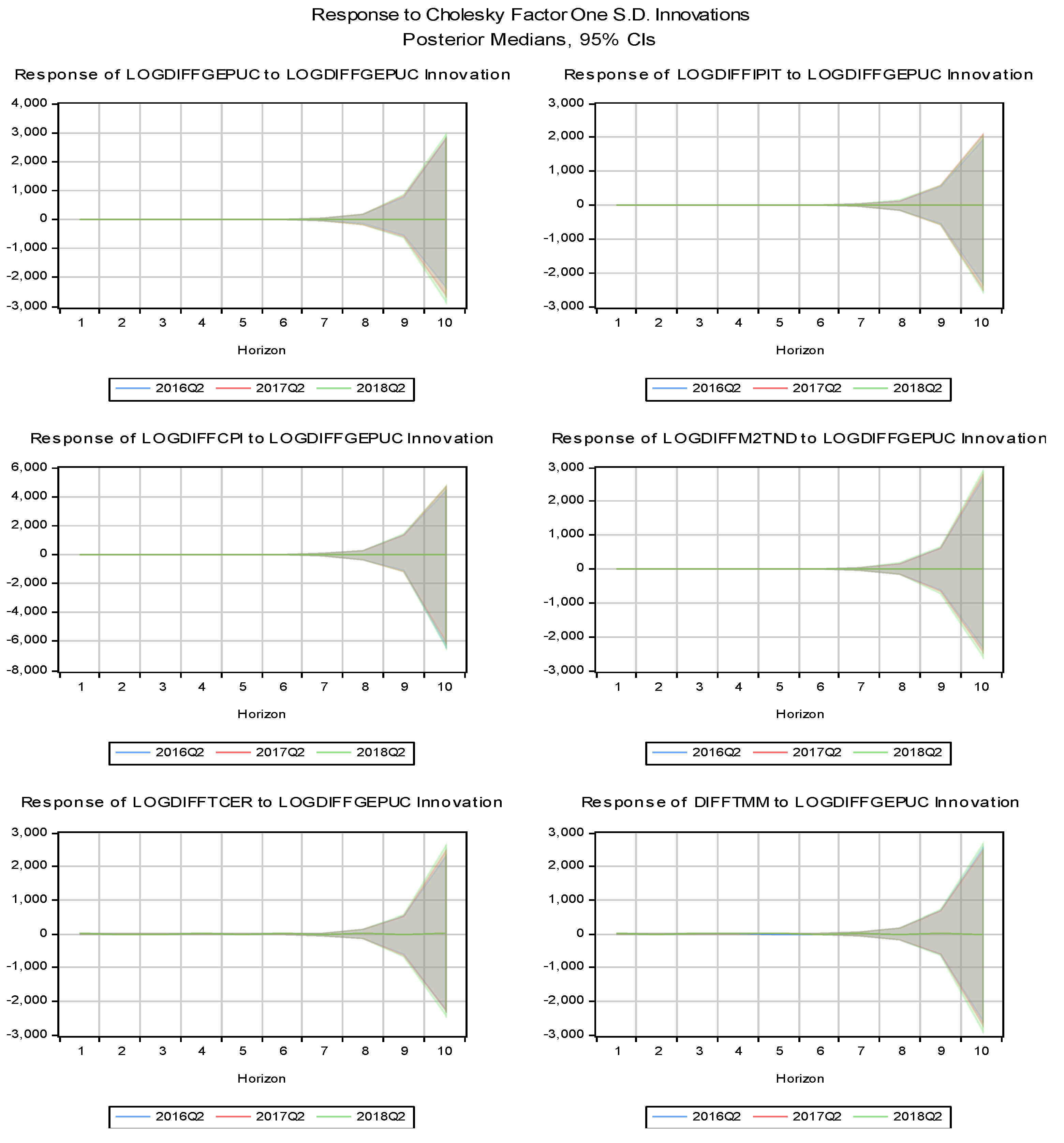
Figure 1 shows impulse response functions (IRFs) from a Bayesian TVC-VAR model. Specifically, these IRFs represent how the Tunisian macroeconomic variables respond to a one standard deviation shock in the global economic policy uncertainty (LOGDIFFGEPUC) over different time horizons (e.g., 4, 8, and 12 quarters) following Nakajima et al. (2011).

• Industrial production:

In the short term (0-4 quarters), the shock of global economic policy uncertainty (LOGDIFFGEPUC) leads to a decline in industrial production (LOGDIFFIPIT). The uncertainty could reduce external demand and investor confidence and lead to a decline in output. Medium-term (4-8 quarters): The effect remains negative but begins to stabilize, suggesting that industrial production is slowly adjusting to the uncertainty shock. In the longer term (8-12 quarters), the impact appears to fade as the economy recovers from the initial shock.

• The consumer price index:

In the short term, the uncertainty shock (LOGDIFFGEPUC) initially causes prices to drop, possibly due to decreased demand or lower commodity prices. In the medium term, prices stabilize as the economy adjusts. There is little further impact on inflation in the long term, though the stabilization takes a while to become apparent.

• Money supply:

In the short-term, a shock in global uncertainty (LOGDIFFGEPUC) leads to a temporary increase in money supply (LOGDIFFM2TND), as central banks may try to provide liquidity to counteract negative effects. In the medium term, the effect continues to rise as more liquidity is injected into the system. The effect stabilizes and eventually declines as monetary policy tightens or adjusts to the external uncertainty several quarters later.

• The money market rate:

Money market rates (DIFFTMM) rise in the short term as a result of the shock, reflecting either higher risk premiums or tighter credit conditions. Interest rates reach their peak and start to level off in the medium term. Rates become more neutral in the long run.

• The real effective exchange rate:

An uncertainty shock results in a short-term increase in the real exchange rate (LOGDIFFTCER). This might be the result of decreased imports, which would strengthen the local currency, or capital inflows looking for safety. The real exchange rate stabilizes over the medium term. A few quarters after the initial capital inflows or adjustments normalize, there might be some reversion.

In summary, industrial production sharply declines in response to a shock in current global economic policy uncertainty, driven by immediate drops in external demand and increased investor uncertainty. This decline is most pronounced in the short term (0–4 quarters). Over the medium to long term (8–12 quarters), production begins to recover, though this recovery may be hindered by ineffective monetary policy tools like the money market rate. In response to uncertainty shocks, monetary authorities may temporarily increase the money supply to mitigate adverse effects. However, money market rates prove ineffective in stimulating industrial production. Higher risk premiums and tighter credit initially raise money market rates, but these do not significantly support production as financial markets adjust. This illustrates the limited impact of monetary policy during high uncertainty, particularly when businesses and consumers are risk-averse. Deflationary forces exert downward pressure on inflation in the short term, while prices stabilize over time. The real effective exchange rate rises sharply initially—likely due to reduced import demand and increased safe-haven capital inflows—before normalizing in the medium to long term. This highlights the challenges monetary policy faces in addressing uncertainty-driven disruptions.

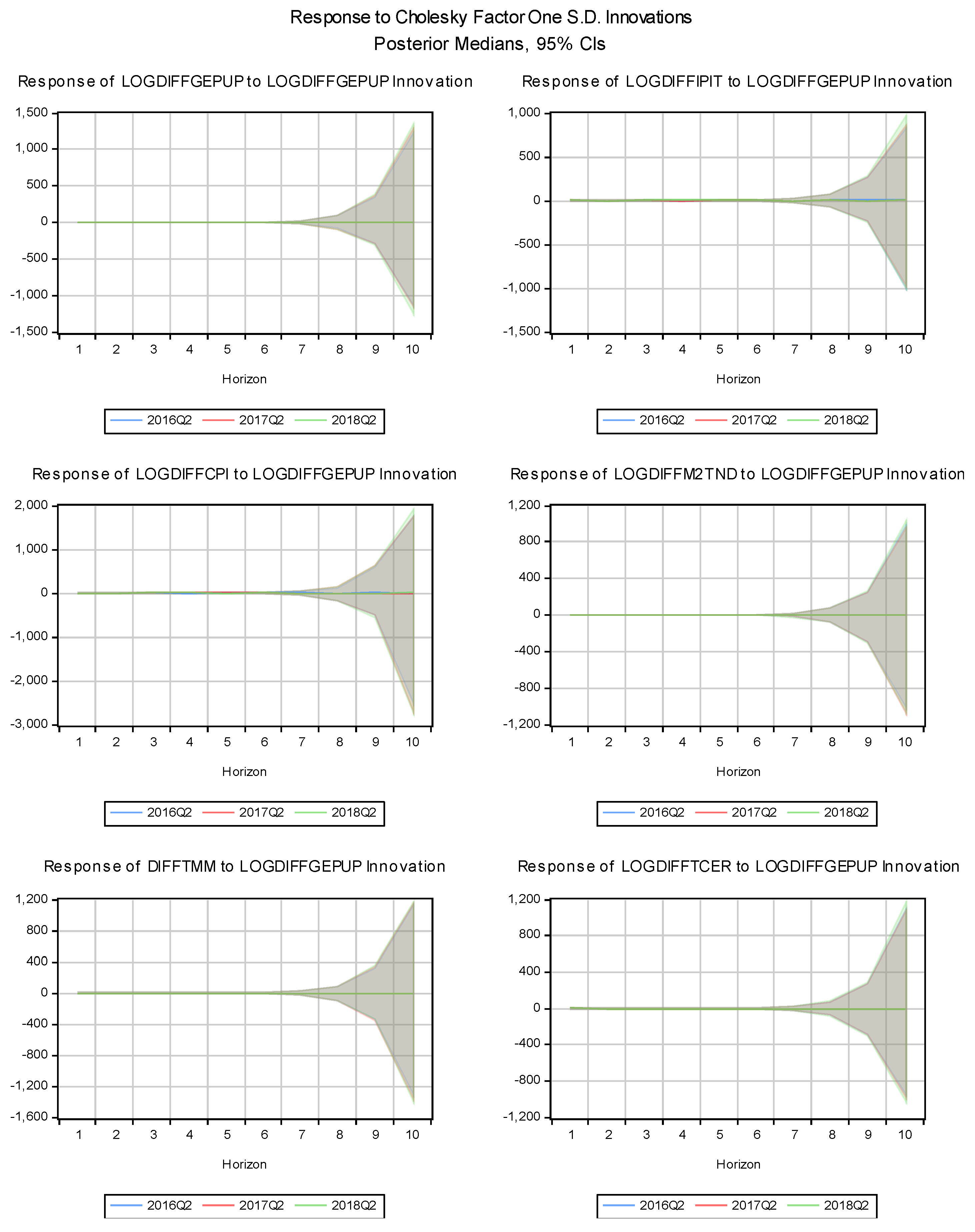
The impact of LOGDIFFGEPUP leads to gradual and prolonged effects (Figure 2). Industrial production (LOGDIFFIPIT) adjusts slowly, showing a delayed response to past uncertainties. The output contraction is prolonged, highlighting the lasting influence of previous uncertainty shocks. Inflation (LOGDIFFCPI) is experiencing a delayed decline amid rising deflationary pressures. The money supply expansion (LOGDIFFM2TND) in response to past uncertainties is more measured than for current uncertainties, reflecting a cautious monetary policy. The money market rate rises gradually, indicating that financial markets take longer to adjust to past uncertainties. This slow adjustment emphasizes the money market rate (potential) ineffectiveness in stimulating production during prolonged uncertainty, as businesses and consumers remain risk-averse and slow to respond to interest rate changes. The real effective exchange rate appreciates slowly as the economy adjusts to past uncertainties affecting trade and capital flows. Current uncertainty prompts swift responses, while past uncertainty leads to prolonged effects. This highlights differing transmission mechanisms, with the money market rate being less effective in mitigating the lasting impacts of past uncertainty on industrial production and economic dynamics.

3.4.2. Response of the Macroeconomic Variables to a Shock in World Uncertainty

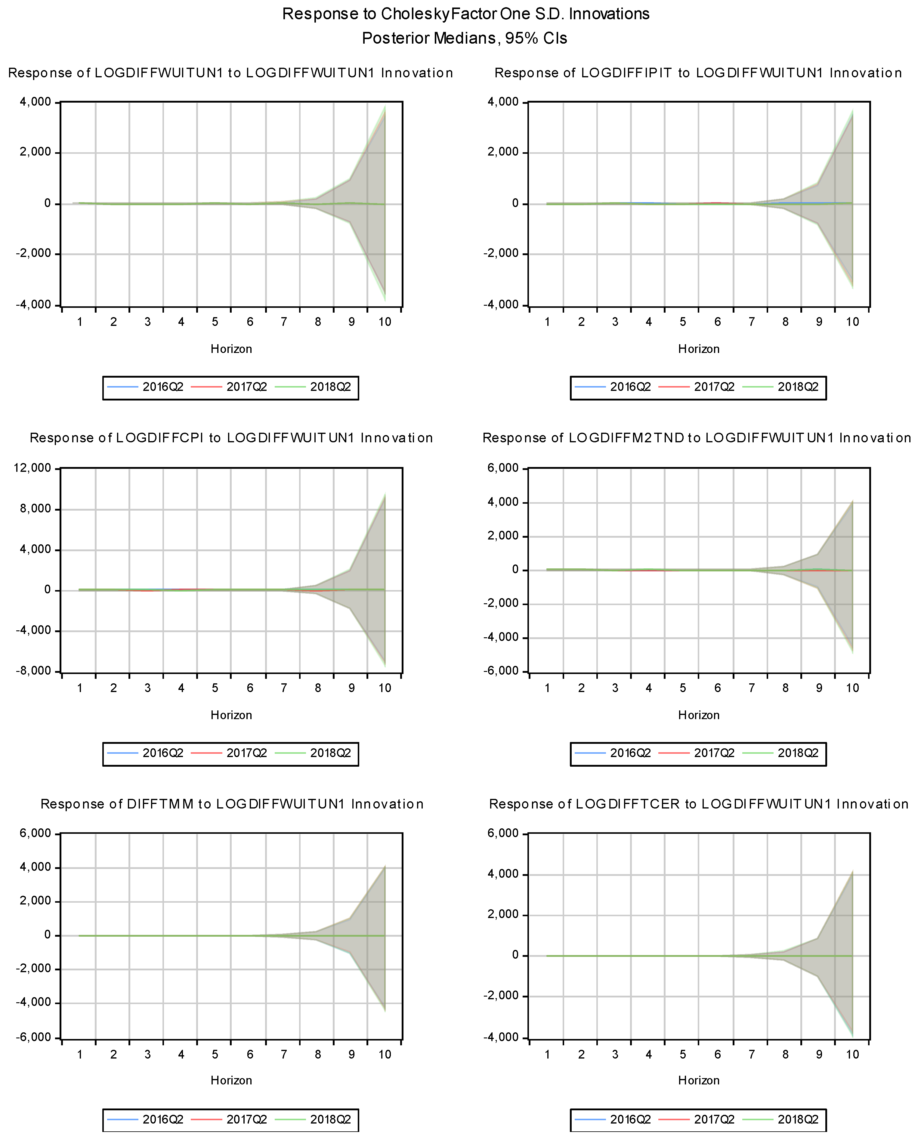
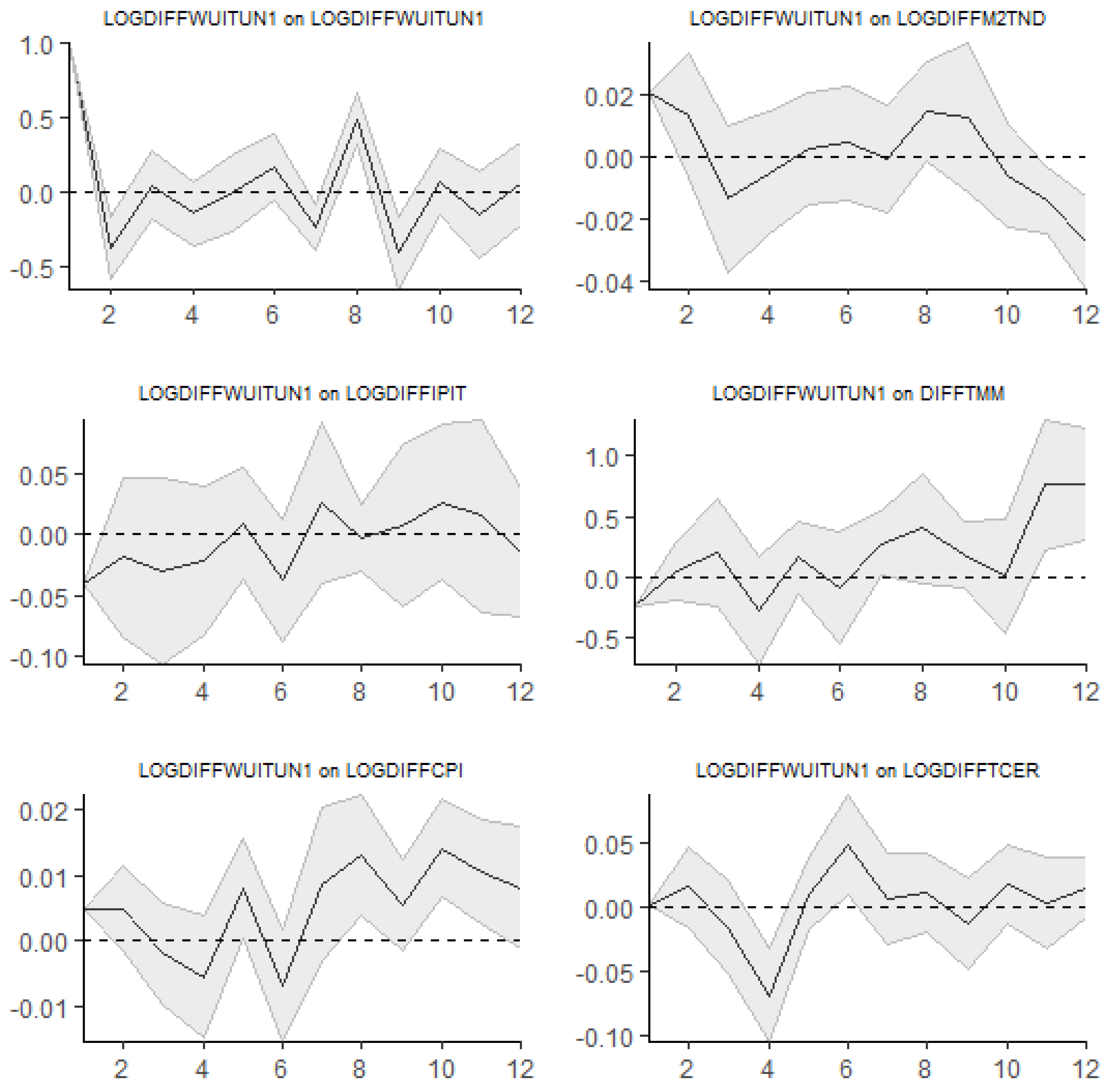
Figure 3 presents the IRFs from a Bayesian TVC-VAR model for Tunisia, where the same macroeconomic variables react to a shock in the World Uncertainty Index for Tunisia, denoted as LOGDIFFWUITUN1.

• Industrial production:

The industrial production index shows a delayed positive response to a shock in the Word uncertainty (LOGDIFFWUITUN1). Over different time horizons (4, 8, and 12 quarters), the reaction becomes more pronounced. At longer horizons (10 quarters), the confidence intervals widen, indicating more uncertainty about future outcomes.

• The consumer price index:

The consumer price index (LOGDIFFCPI) exhibits an initially flat response but shows an increasingly positive response after 6 quarters. This suggests that higher world uncertainty (LOGDIFFWUITUN1) eventually leads to higher inflationary pressures in Tunisia. The expanding confidence bands highlight increasing uncertainty in price estimates over time.

• Money supply:

The monetary aggregate (LOGDIFFM2TND) exhibits a slow initial response before gradually declining over eight to ten quarters. Possibly as a result of the central bank's attempts to lessen the effects of global uncertainty, this suggests a tightening of monetary conditions.

• The money market rate:

The money market rate (DIFFTMM) exhibits a slow initial response before progressively declining. Accordingly, there isn't likely to be a major change in monetary policy shortly, but as uncertainty (LOGDIFFWUITUN1) increases and economic activity slows, rates may eventually be reduced.

• The real effective exchange rate:

Over extended periods, the real effective exchange rate (LOGDIFFTCER) responds negatively. This implies that increased uncertainty around the world causes the Tunisian dinar to depreciate. Around the 10-quarter horizon, the effect becomes more noticeable.

The IRFs show that the Tunisian economy is highly vulnerable to global uncertainty shocks from pandemics, crises, and wars. These shocks gradually and persistently affect long-term industrial production, inflation, monetary policy, and exchange rates, with initial effects being muted but intensifying over time. Industrial production often increases over time, possibly due to delayed global demand adjustments or government interventions. Inflation rises, likely from cost-push factors related to heightened uncertainty. Tightening money supply and exchange rate depreciation indicate potential central bank interventions to stabilize the economy during highly uncertain times.

The money market rate is a key monetary policy tool, with the central bank's interest rate adjustments crucial for economic management. However, muted initial responses and delayed effects suggest it may be less effective in stimulating production and stabilizing prices during significant uncertainty, as financial markets and economic agents need time to adjust.

The widening confidence intervals at longer time horizons highlight the growing unpredictability of economic outcomes, posing challenges for monetary policy in responding to prolonged global shocks.

3.4.3. Response of Macroeconomic Variables to a Shock in US Monetary Policy Uncertainty

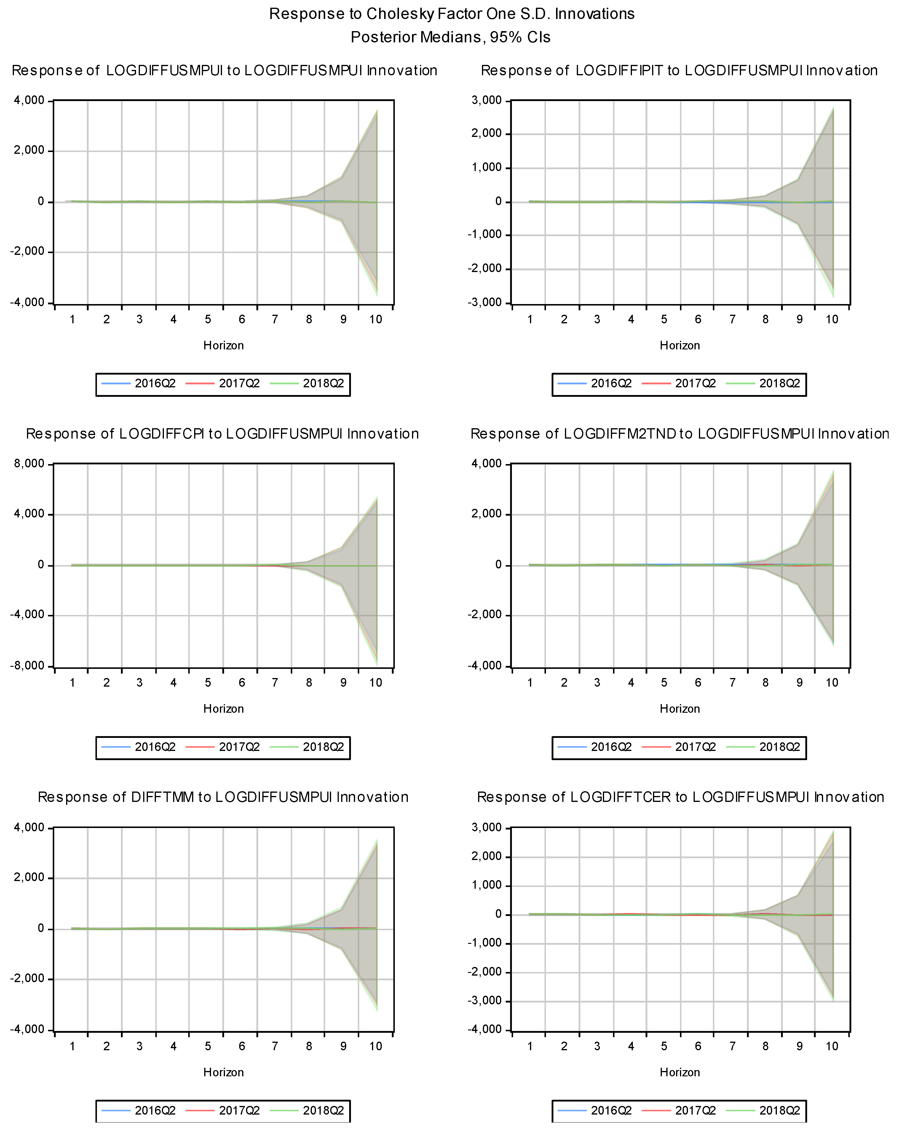
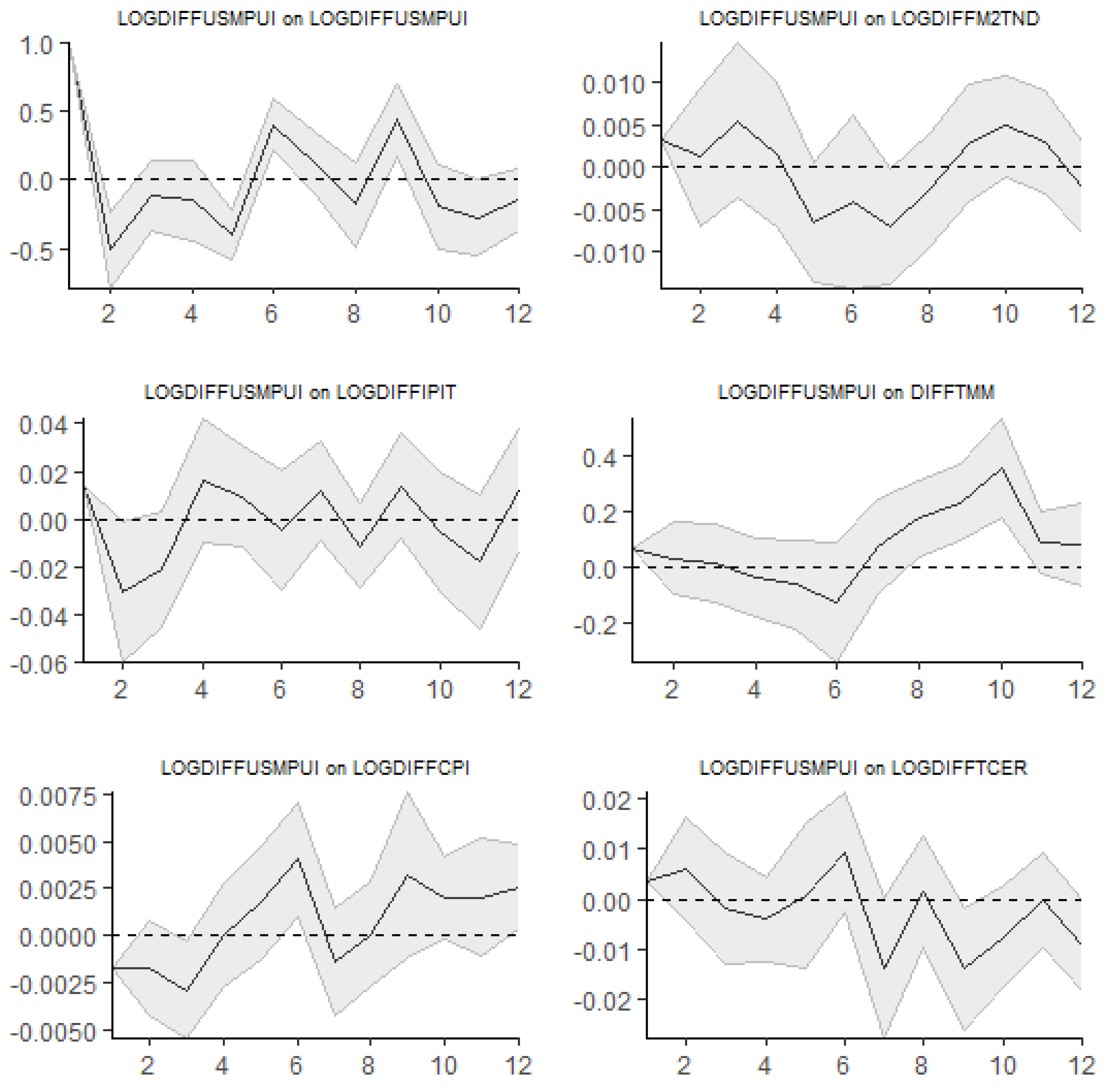
Figure 4 presents the IRFs from a Bayesian TVC-VAR model, showing how various Tunisian macroeconomic variables react to a shock in the US Monetary Policy Uncertainty Index (LOGDIFFUSMPUI). The responses are shown for several macroeconomic variables over different time horizons: 4, 8, and 12 quarters.

• Industrial production:

The industrial production index (LOGDIFFIPIT) in Tunisia shows an increasingly positive response to uncertainty in US monetary policy after about four to six quarters, suggesting that higher uncertainty in US monetary policy (LOGDIFFUSMPUI) could lead to an increase in industrial production in Tunisia in the medium term. This could be due to increased foreign investment or economic adjustments in response to changing external conditions.

• The consumer price index:

The consumer price index (LOGDIFFCPI) shows a lagged but positive response to the shock, suggesting that US monetary policy uncertainty (LOGDIFFUSMPUI) may contribute to inflationary pressures in Tunisia over time. Confidence intervals are widening significantly, reflecting growing uncertainty about inflation outcomes over a longer period.

• Money supply:

The monetary aggregate (LOFDIFFM2TND) reacts negatively after about 6-8 quarters, which may indicate that monetary conditions in Tunisia are tightening due to external monetary uncertainty (LOGDIFFUSMPUI). This tightening could be a response to easing inflationary pressures or stabilizing financial conditions.

• The money market rate:

The money market rate (DIFFTMM) is showing an upward movement after about six quarters, suggesting that Tunisia's interest rates are rising in response to U.S. monetary policy uncertainty (LOGDIFFUSMPUI). This could be due to central bank efforts to stabilize capital flows or prevent capital flight.

• The real effective exchange rate:

The real effective exchange rate (LOGDIFFTCER) shows a negative reaction over the 8-10 quarter time horizon, suggesting that the Tunisian currency is depreciating in response to US monetary policy uncertainty (LOGDIFFUSMPUI). This could be due to capital outflows or declining confidence in the Tunisian economy as global conditions become more uncertain.

In summary, US monetary policy uncertainty significantly impacts Tunisia's economy with a delay. In the short to medium term, industrial production benefits from adjustments in global demand, while long-term effects include inflationary pressures and exchange rate depreciation due to persistent uncertainty. Tunisia's monetary policy, through money supply and interest rate adjustments, counters inflation and maintains financial stability. The money market rate is crucial for managing inflationary pressures, but its effectiveness is delayed by the slow response of financial markets to US monetary policy uncertainty.

US monetary uncertainty has mixed effects on Tunisia’s economy, providing short-term benefits to output while negatively impacting inflation and the exchange rate in the long term. Widening confidence intervals suggest increasing uncertainty about future economic outcomes, complicating Tunisia’s response to uncertainty.

3.4.4. Response of Macroeconomic Variables to a Shock in US Financial Stress

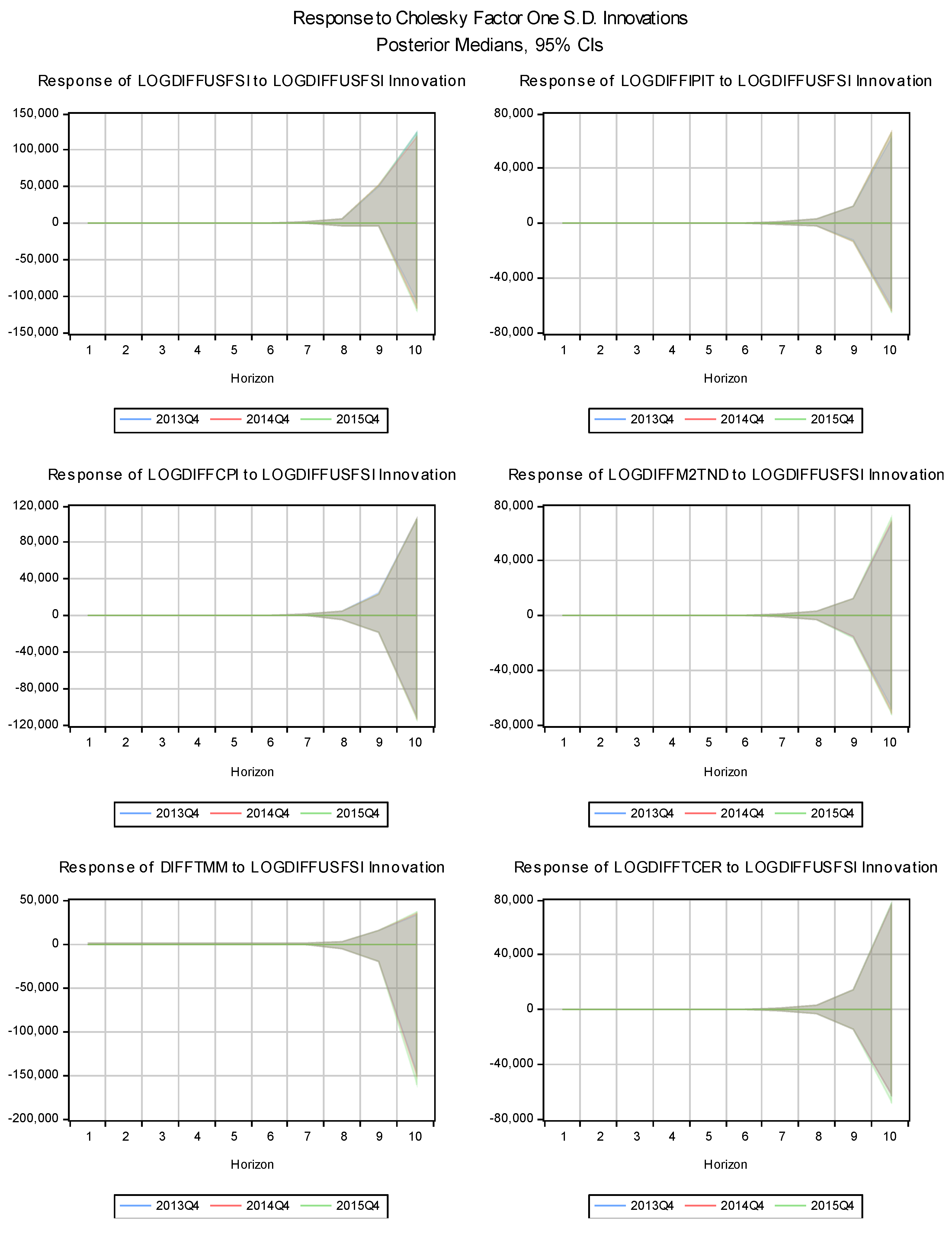
Figure 5 displays the IRFs from a Bayesian TVC-VAR model, illustrating how Tunisia’s key macroeconomic variables react to a shock in the US Financial Stress Index (LOGDIFFUSFSI). The responses are tracked over different time horizons (4, 8, and 12 quarters), providing insights into Tunisia’s vulnerability to US financial stress.

• Industrial production:

Industrial production (LOGDIFFIPIT) reacts with a delay but increasingly to the shock, with a noticeable increase after 6 to 8 quarters. This suggests that the growing financial crisis in the US could have a positive impact on Tunisia's industrial production in the medium term, possibly driven by shifts in global capital flows or changes in external demand.

• The consumer price index:

The consumer price index (LOGDIFFCPI) reacts positively, although with a slight delay. After about eight quarters, inflation begins to rise, suggesting that financial stress in the US (LOGDIFFUSFSI) is leading to inflationary pressures in Tunisia. This could be due to imported inflation or higher borrowing costs as global financial conditions tighten.

• Money supply:

The monetary aggregate (LOGDIFFM2TND) shows an increasing response after six quarters, reflecting an increase in liquidity in the financial system. This could be due to domestic monetary policy adjustments to counteract the impact of external financial stresses by increasing liquidity to support economic activity.

• The money market rate:

The money market rate (DIFFTMM) remains relatively stable in the short term but shows an upward reaction over time. This suggests that interest rates in Tunisia are rising following the financial stress in the US (LOGDIFFUSFSI), likely due to a tightening of domestic monetary policy to prevent capital outflows or inflationary spirals.

• The real effective exchange rate:

The real effective exchange rate (LOGDIFFTCER) experiences a long-term depreciation, which increases after 8 quarters. This suggests that financial stress in the US (LOGDIFFUSFSI) is weakening Tunisia's currency, possibly due to lower investor confidence or capital flight from emerging markets such as Tunisia.

A shock to the US financial stress index significantly and gradually affects the Tunisian economy. Initially, industrial production benefits due to global demand adjustments and delayed responses from the government or businesses. However, this stability is accompanied by rising inflation and increased liquidity as the central bank adjusts the money supply in response to external pressures.

While the initial economic boost may seem beneficial, the effectiveness of Tunisia's monetary policy tools, especially the money market rate, is evident. The central bank's adjustments to money supply and interest rates aim to stabilize the economy, but the money market rate struggles during external financial stress. Its delayed adjustment reflects its limited ability to respond quickly to US financial tensions, which led to higher domestic interest rates and a depreciation of the real effective exchange rate.

These responses highlight the interconnectedness of global financial markets and Tunisia’s vulnerability to external shocks. The money market rate, as a monetary policy tool, is less effective in mitigating external stress, particularly when financial markets are slow to adjust. The depreciation of the exchange rate and rising interest rates show how Tunisia’s monetary policy can be overwhelmed by external shocks, resulting in a misalignment between domestic measures and external economic realities.

Tunisia’s central bank can manage some immediate effects through liquidity adjustments; however, the broader economic impact of U.S. financial stress reveals the limitations of the money market rate in stabilizing the economy during high external volatility. This suggests that Tunisia may need to supplement traditional monetary policy with fiscal interventions or enhanced financial market actions to address prolonged external uncertainty.

3.4.5. Response of Macroeconomic Variables to Oil Price Uncertainty

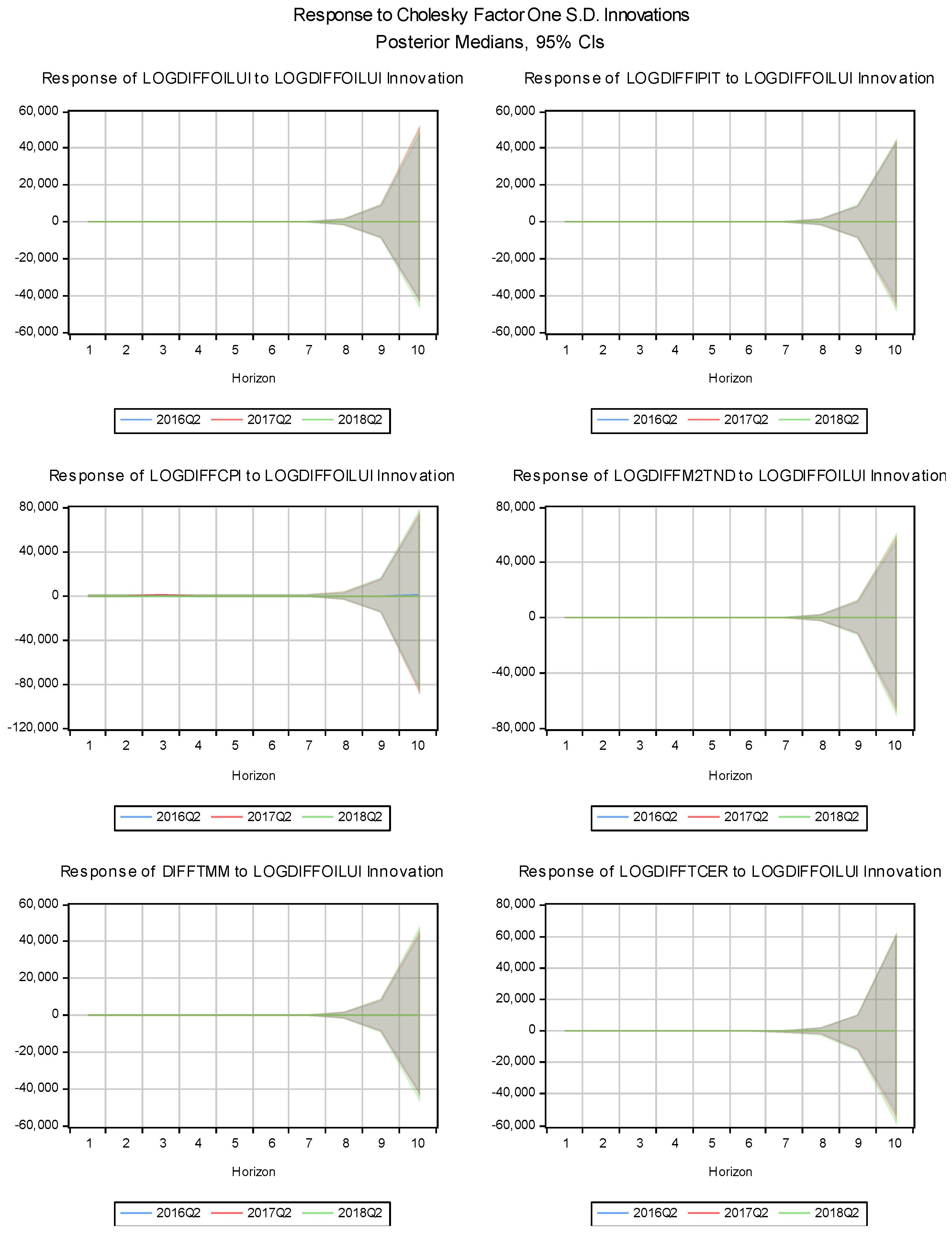
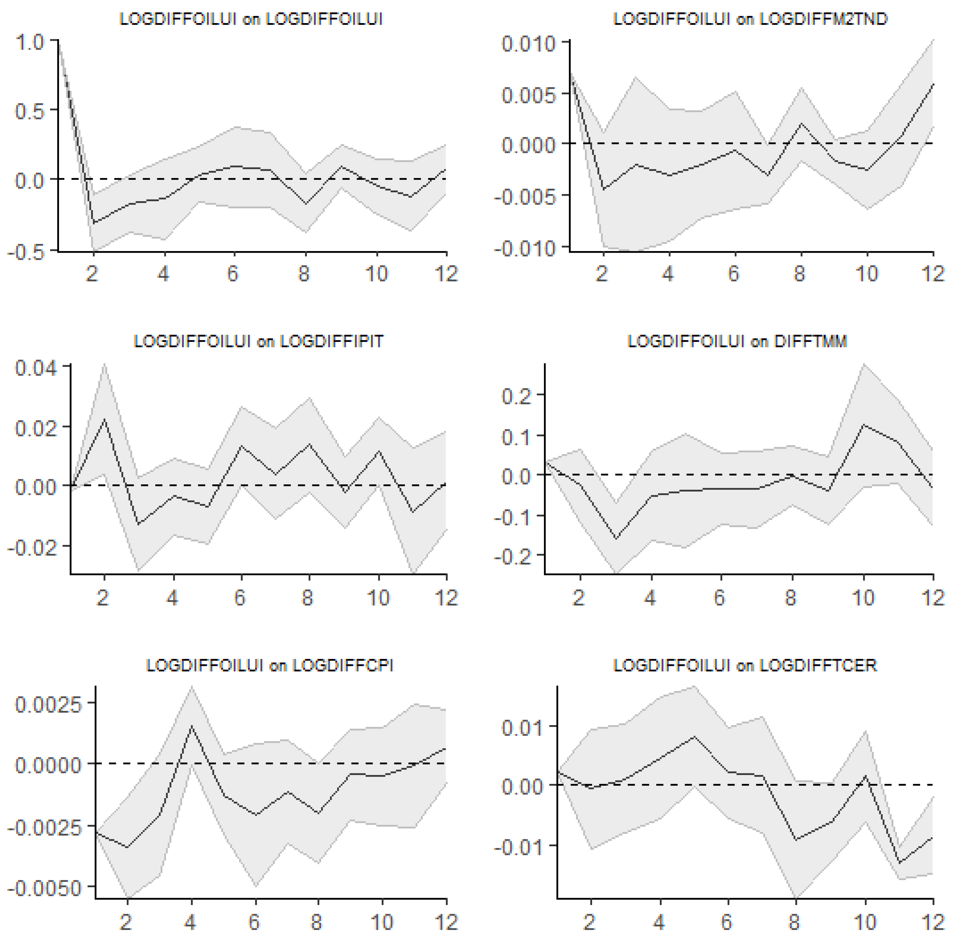
Figure 6 shows the impulse responses from a Bayesian TVC-VAR model, illustrating how different economic variables in Tunisia respond to a shock in the Oil price Uncertainty Index (LOGDIFFOILUI) over time. Each graph tracks these responses at different horizons (4, 8, and 12 quarters ahead).

• Industrial production:

The reaction of industrial production (LOGDIFFIPIT) is initially close to zero but becomes negative over time. This suggests that oil price uncertainty (LOGDIFFOILUI) is harming industrial production in Tunisia, with increasing impacts over the forecast period.

• The consumer price index:

The consumer price (LOGDIFFCPI) also shows a lagged positive response to oil price uncertainty. This means that uncertainty about oil prices creates inflationary pressures, driving up consumer prices over time.

• Money supply:

The money supply response (LOGDIFFM2TND) is initially slightly positive and increases over time, suggesting that monetary authorities may respond to oil price uncertainty by expanding the money supply.

• The money market rate:

The money market interest rate (DIFFTMM) shows a lagged negative response, suggesting that uncertainty in oil prices (LOGDIFFOILUI) may lead to lower interest rates as a monetary policy measure to support economic activity.

• The real effective exchange rate:

The exchange rate (LOGDIFFTCER) initially shows a minimal reaction. It eventually increases, suggesting that uncertainty about the oil price (LOGDIFFOILUI) could lead to a real increase in the value of the Tunisian currency over time.

To sum up, increased oil price uncertainty leads to a sustained decline in industrial production, highlighting its negative impact on economic activity. This downturn dampens business confidence, reduces investment, and disrupts production processes. The decline underscores the importance of energy costs in shaping industry competitiveness and operational efficiency, especially in Tunisia's economy, which is vulnerable to external shocks.

This uncertainty coincides with rising consumer prices, indicating inflationary pressures likely driven by higher energy import costs. The increase reflects the direct impact of expensive oil and heightened inflation expectations. As oil price volatility escalates, businesses and consumers may adjust their pricing behaviors, further exacerbating inflation. This illustrates how oil price uncertainty affects immediate production costs and alters broader economic expectations.

Monetary authorities are expanding the money supply to inject liquidity and mitigate the adverse effects of the oil price shock. This aims to counteract the contraction in industrial output and alleviate inflationary pressures from rising energy prices. However, the effectiveness of this policy is limited by the money market rate's ability to manage external shocks.

The decline in the money market rate indicates that the central bank is cutting interest rates to stimulate economic growth and investment. However, during periods of high uncertainty, financial markets may respond slowly to these changes. Investors may be cautious, and businesses may delay production expansion despite lower borrowing costs. Thus, the money market rate's ability to drive a timely recovery in industrial production may be limited, especially if oil price uncertainty persists.

The real effective exchange rate rises after the oil price shock, likely due to capital inflows into Tunisian assets or currency adjustments from global oil market volatility. This domestic currency depreciation may reflect a broader rebalancing of financial flows in response to oil price changes and global economic conditions.

Oil price uncertainty is dampening industrial production in Tunisia and fueling inflation. The slow adjustment of financial markets to policy changes reveals the money market rate's potential ineffectiveness in addressing oil price uncertainty.

3.5. Results of LPs

The impulse response functions of linear local projections are displayed in Figure 7, Figure 8, Figure 9, Figure 10, Figure 11 and Figure 12. Each graph shows the impact of uncertainty variable shocks on the macroeconomic variables.

3.5.1. Impact of Global Economic Policy Uncertainty Shocks on Macroeconomic Variables

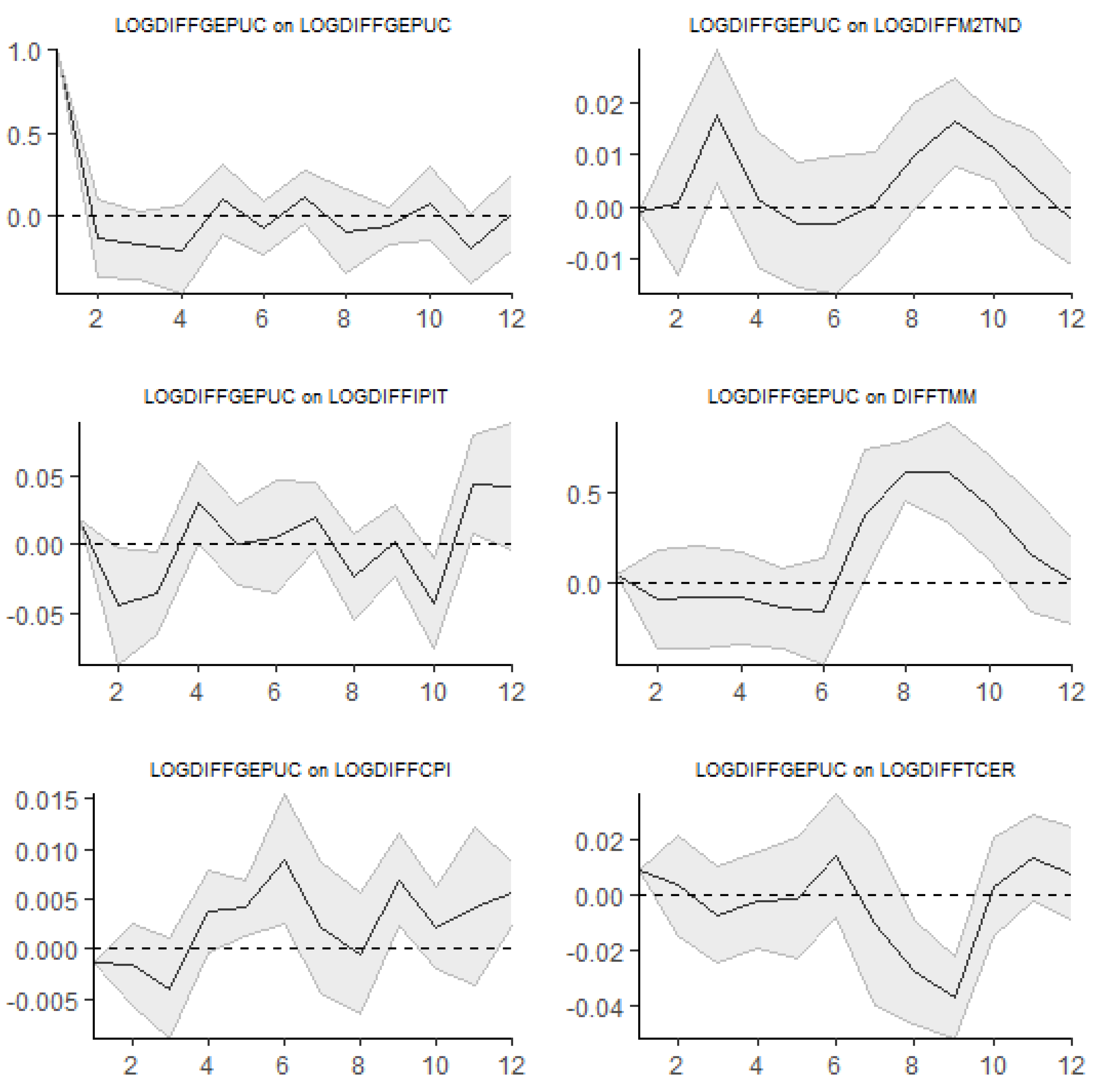
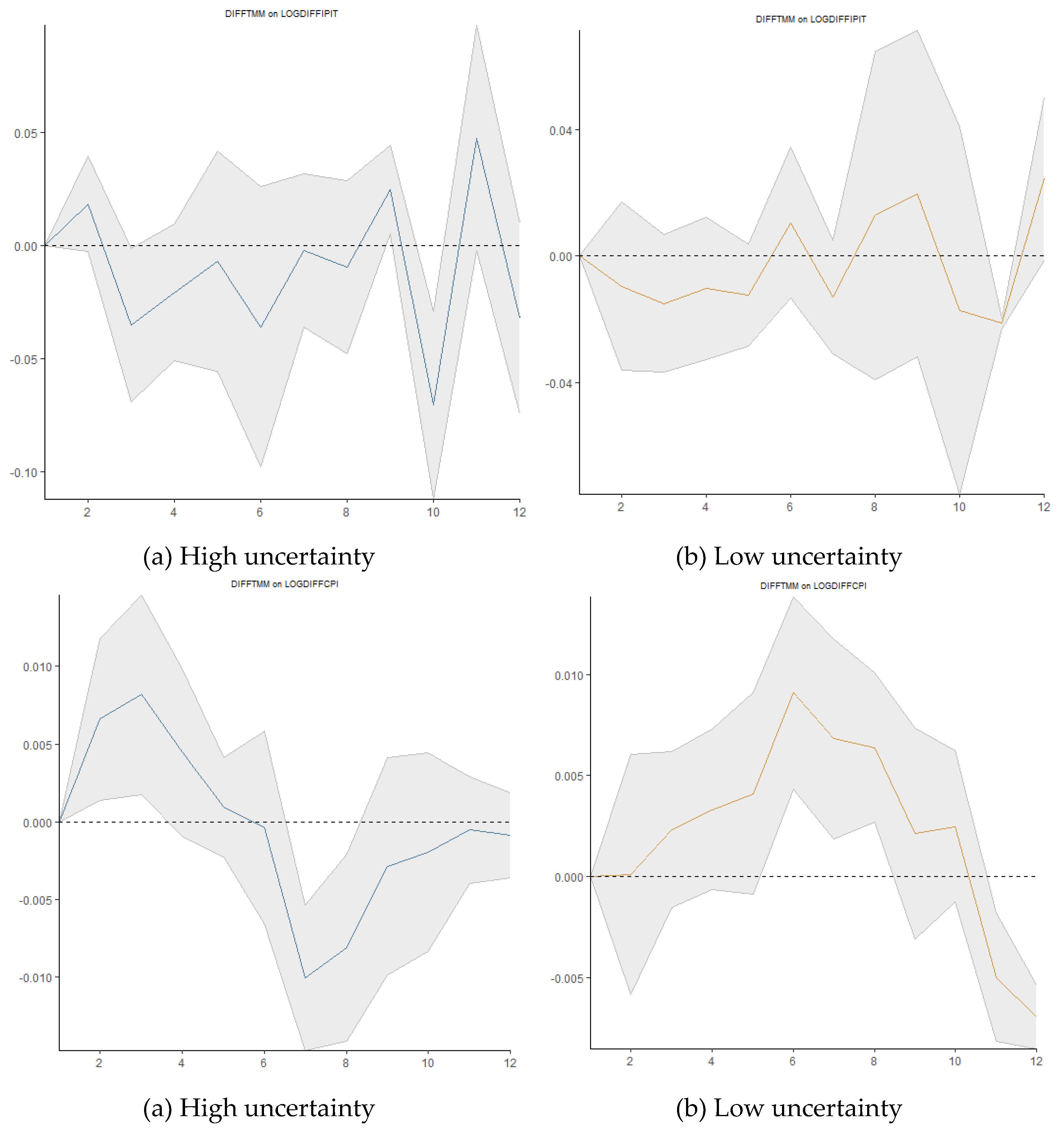
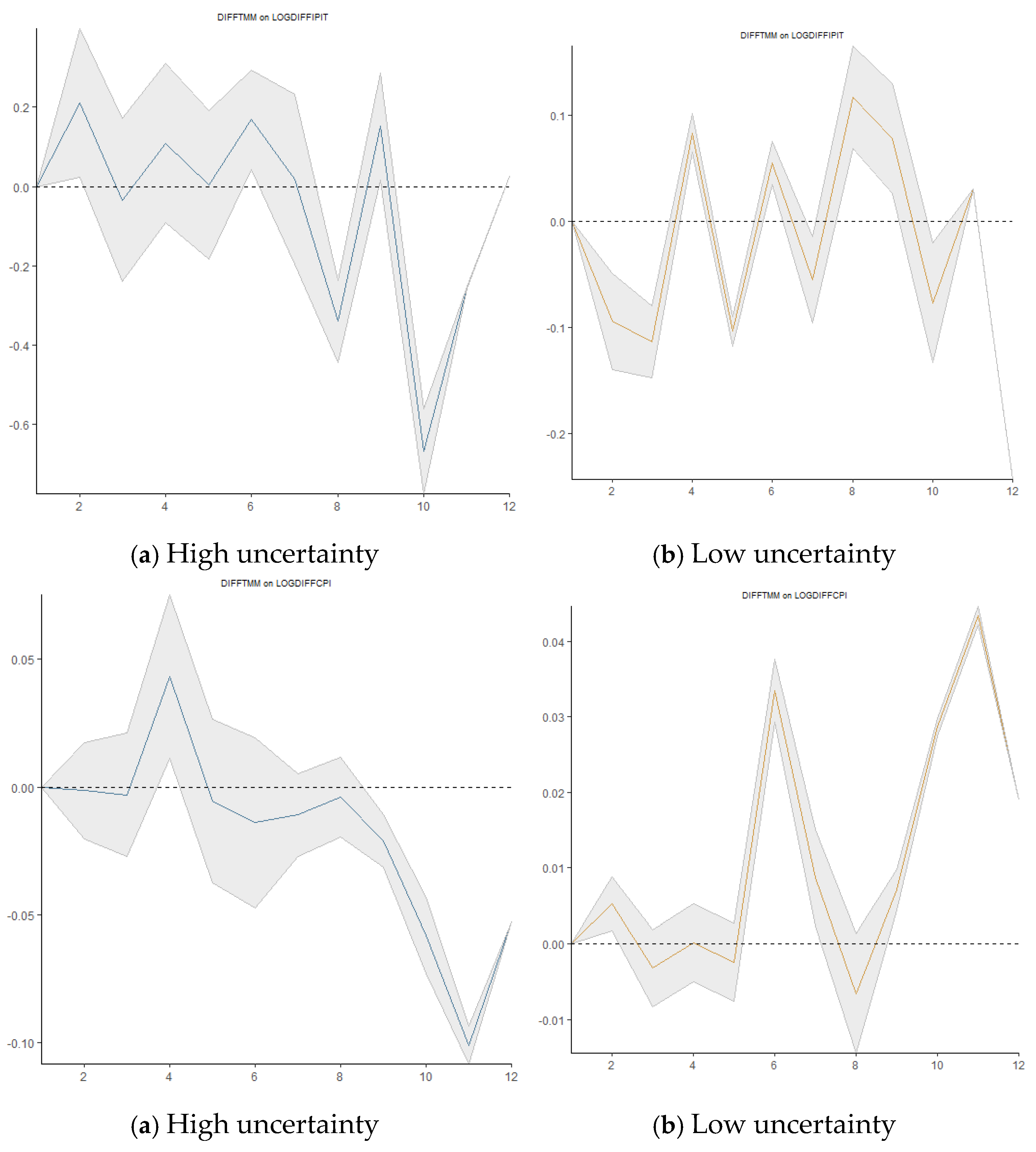
Figure 7 shows the impulse responses based on local linear projections, all identified with a standard Cholesky decomposition and the causal order (industrial production, consumer price index, money supply, money market rate, real exchange rate, and the global economic uncertainty variable). According to Trabelsi and Ben Khaled (2023). We use AIC to select the optimal delay (p) with a maximum set to 8. The solid line and the two thick lines show the responses from LPs and the corresponding Newey-West corrected two standard error bands. The LP response of industrial production (LOGDIFFIPIT) and inflation (LOGDIFFCPI) suggests a 0.025% increase to a shock in the GEPUC 12 quarters after the impact. The money supply's response to the increase in LOGDIFFGEPUC exhibits both positive and negative effects, remaining statistically insignificant over 12 quarters. The LPs show a negative initial money market reaction (DIFFTMM) with a dramatic increase around the seventh quarter. The response of the real effective exchange rate (LOGDIFFTCER) to the global economic uncertainty shock is unstable but tends to decline 12 quarters later.

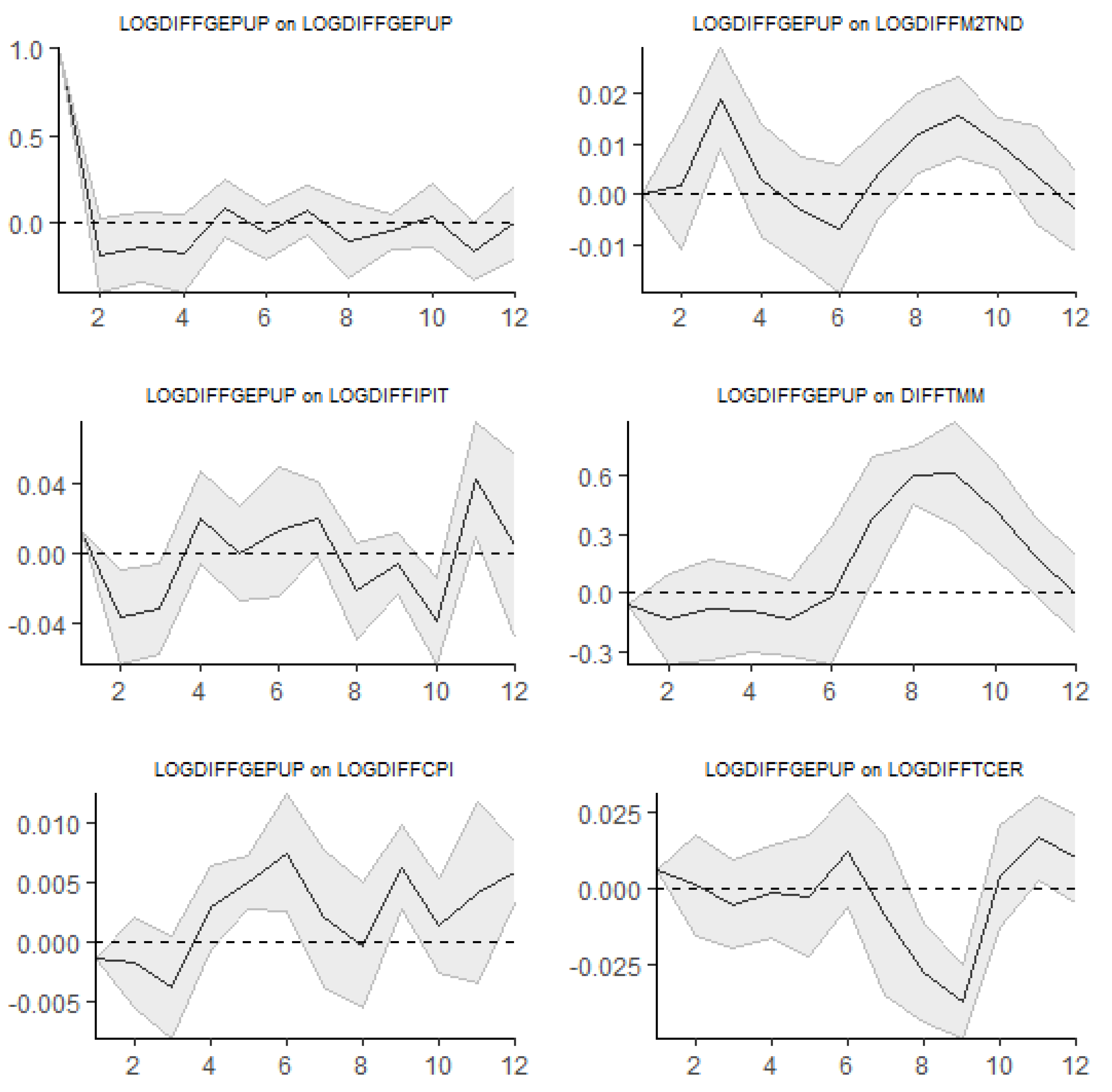
If we replace the uncertainty variable with LOGDIFFGEPUP, the results in Figure 8 are almost identical to the previous ones. Global economic uncertainty can disrupt monetary policy transmission, affecting output and inflation, particularly when economic agents ignore central bank announcements.

3.5.2. Impact of the World Uncertainty Shocks on Macroeconomic Variables

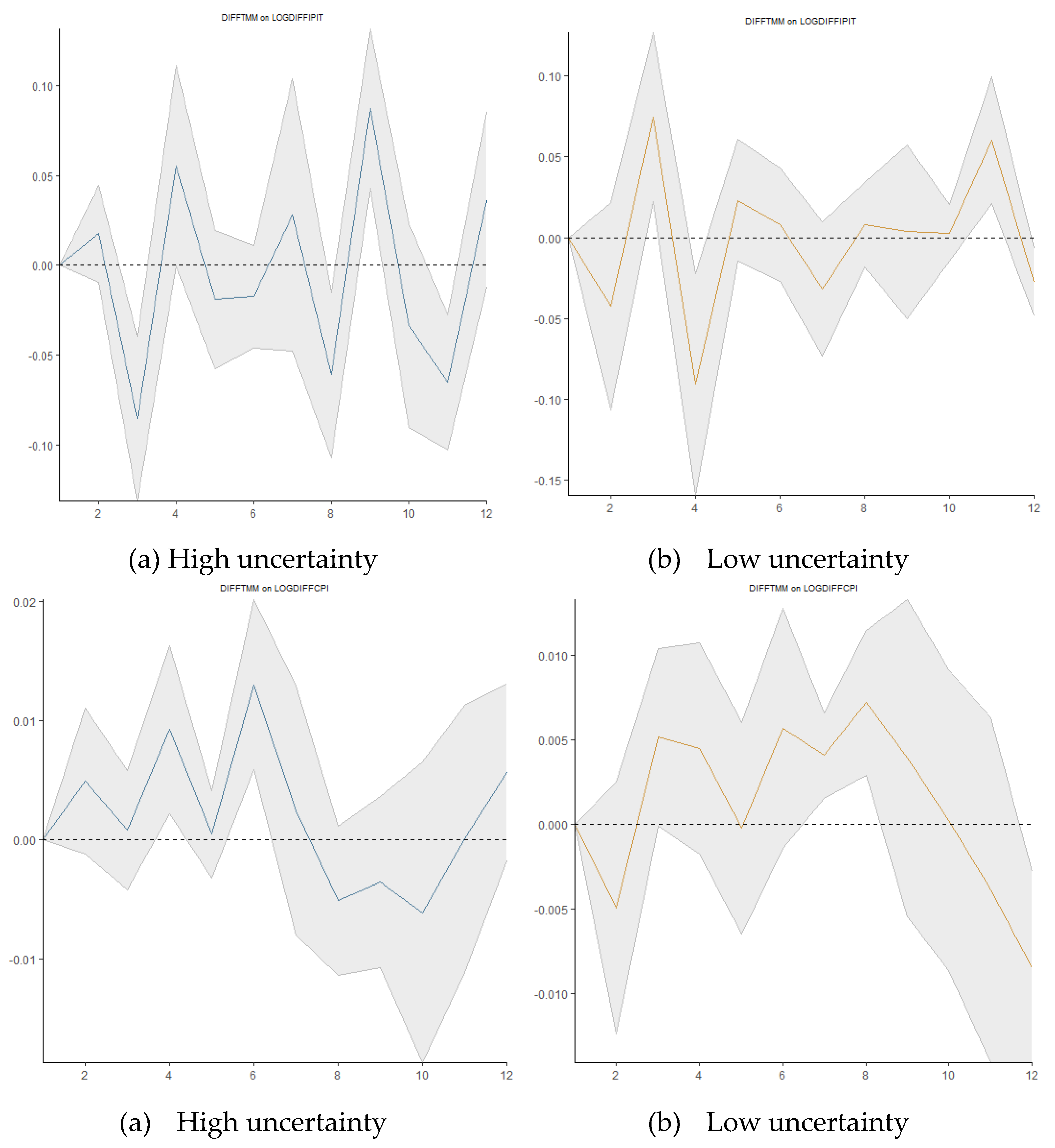
The money market rate and the real effective exchange rate have a positive correlation with an increase in the World Uncertainty Index shock starting in the seventh quarter. The money supply, inflation, and industrial production usually decrease twelve quarters later (Figure 9). An industrial production contraction (LOGDIFFIPT) is usually the result of a shock to global uncertainty because of delayed investments, weakened global demand, and disrupted supply chains. Inflation (LOGDIFFCPI) also decreases as a result of less demand pushing down prices. The real exchange rate (LOGDIFFTCER) may also decline as a result of these shocks, increasing Tunisia's export competitiveness while also driving up import prices. The central bank of Tunisia frequently responds by increasing the money supply (LOGDIFFM2TND) to supply liquidity and lowering the money market rate (DIFFTMM) to encourage borrowing and boost the country's economy. Global uncertainty generally has a stabilizing effect on inflation but a destabilizing effect on output. Pandemic, war, and crisis-related uncertainty make investors fearful and increase their vigilance until they have more accurate information to react to changes in policy. This aligns with the opinions of Trabelsi and Serghini (2024), who compared the actions of the private sector before and during the COVID-19 pandemic.

3.5.3. Impact of US Monetary Policy Uncertainty Shocks on Macroeconomic Variables

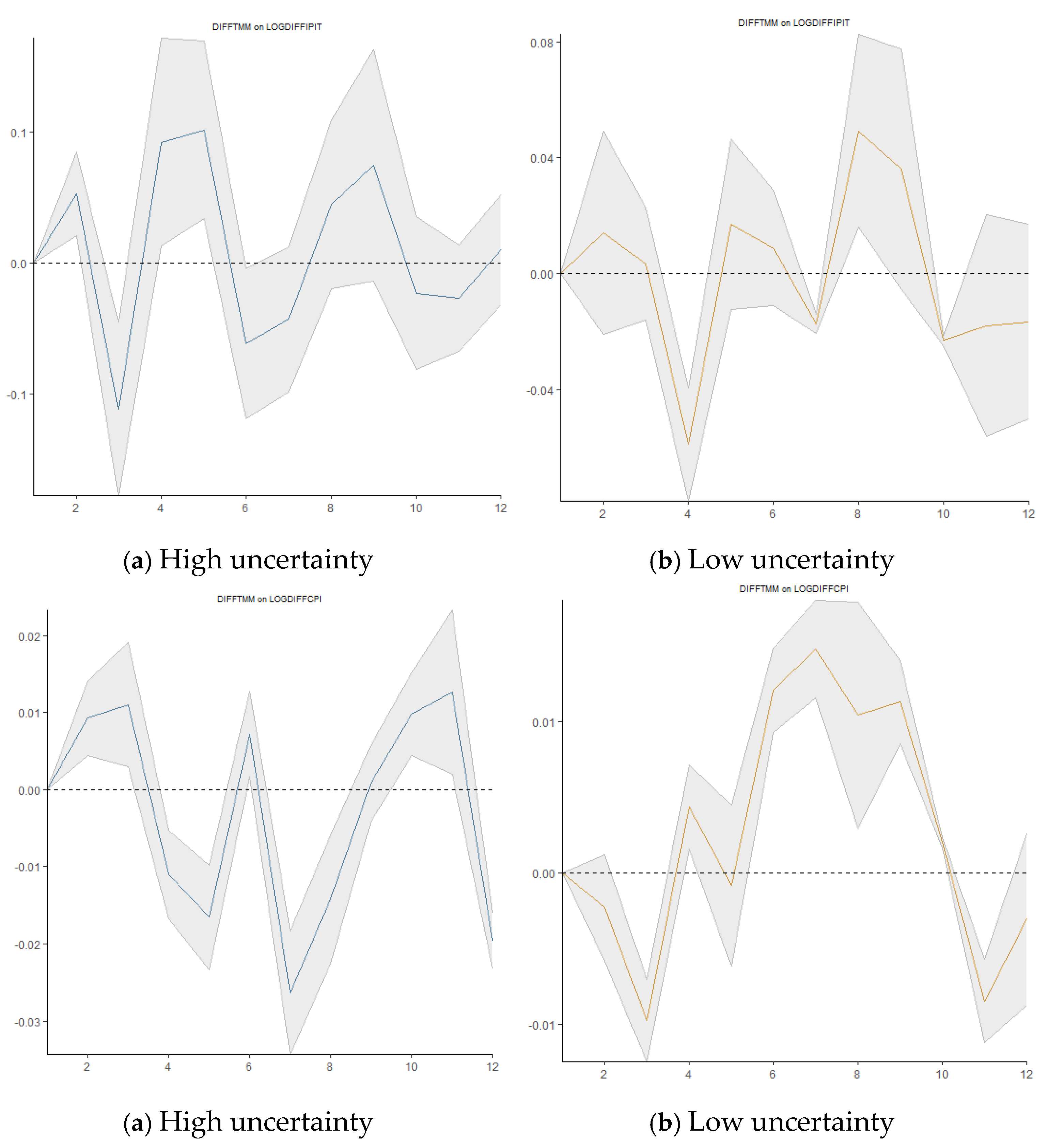
The impact of the same shock on the real effective exchange rate pertains to be negative over a long horizon. We are interested in how the same basket of variables reacts to a shock in the US monetary policy uncertainty (LOGDIFFUSMPUI), with a focus on spillover uncertainty shocks. The most noticeable effect is seen in the money market rate (DIFFTMM) and inflation (LOGDIFFCPI) responses, which after seven quarters show an upward trend albeit one that is unstable (Figure 10). Twelve quarters after a shock to the US monetary policy, the money supply and industrial production respond less uncertainly. Over an extended period, the same shock is likely to hurt the real effective exchange rate.

3.5.4. Impact of US Financial Stress Shocks on Macroeconomic Variables

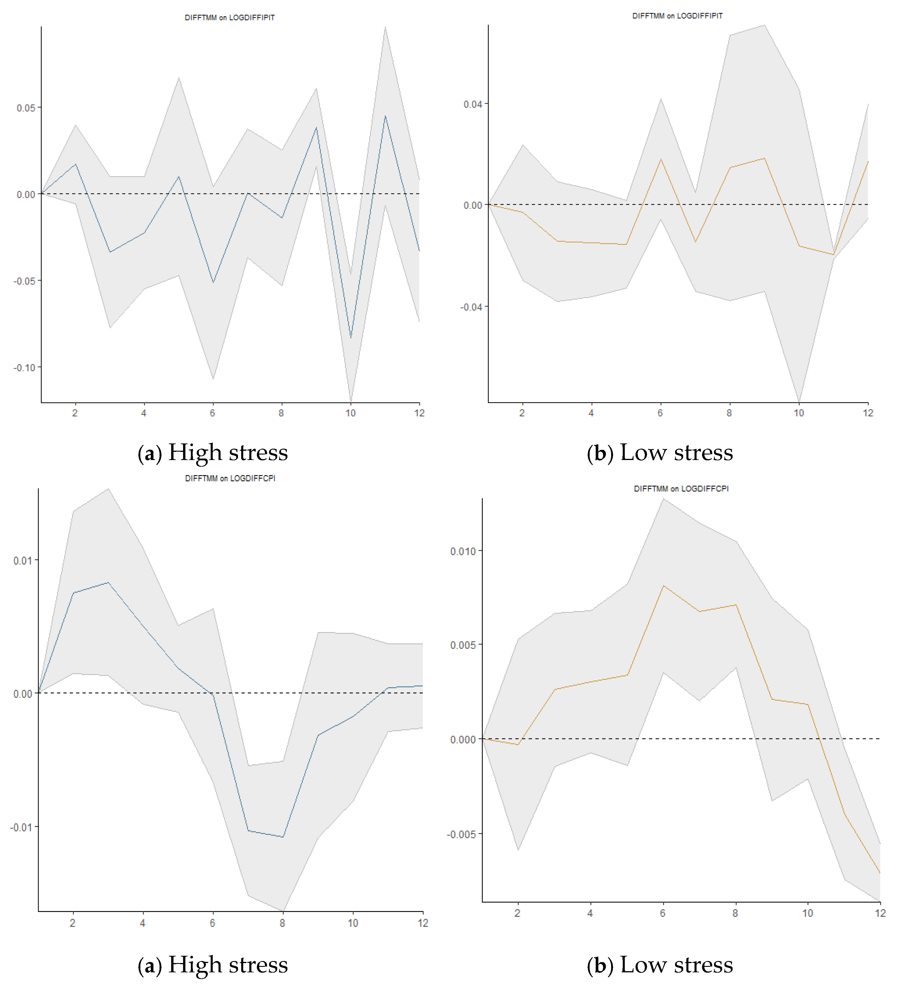
An increase in the US financial stress index causes a rise in the consumer price index (LOGDIFFCPI) from the eighth quarter and in the money supply seven quarters afterward before decreasing again in the remaining quarters. We observe a dramatic decline in the money market rate (DIFFTMM) due to the shock while the response of the real effective exchange rate (LOGDIFFTCER) is downward but remains positive in the last quarters. There is an appreciation of the local money compared to the US dollars of about 1% (see Figure 11).

The production and financial markets of Tunisia are particularly strained by the tighter global credit conditions brought on by US monetary policy uncertainty (LOGDIFFUSMPUI) and financial stress (LOGDIFFUSFSI). Interest rate reductions and monetary expansion that eventually become contraction are the CBT's responses to negative external effects. It takes time for economic agents to assimilate effective and transparent information regarding monetary policy positions.

3.5.5. Impact of Oil Price Uncertainty Shocks on Macroeconomic Variables

The consumer price index, money market rate, and money supply all rise in response to an oil price uncertainty shock (LOGDIFFOILU), particularly in the most recent quarters. The same shock causes the real effective exchange rate (LOGDIFFTCER) to drop precipitously in the tenth quarter before increasing gradually over the following quarters (see Figure 12). Because Tunisia is more dependent on imported energy, oil price uncertainty (LOGDIFFOILUI) has a more direct inflationary effect. It may raise consumer prices, lower industrial output, and further devalue the currency. CBT's monetary policy eases restrictions to ensure economic stability.

3.6. Toda-Yamamoto Granger Causality

Recall that all variables are stationary after the first difference. They are integrated of order 1 (I(1)). We therefore follow the approach of Toda and Yamamoto (1995). The maximum choice of lag order (k) of the VAR for variables in levels is selected according to AIC (see Table S.7 in the supplementary file). We then keep the estimate of the VAR with lag=k+dmax=k+1 and perform the Wald test. We consider a bivariate system in the spirit of Siami-Namini (2017):

$$\left\{\begin{array}{c}{\mathit{Y}}_{\mathit{t}}={\mathit{\alpha }}_{\mathit{Y}}+\sum _{\mathit{i}=1}^{\mathit{k}+\mathit{d}\mathit{m}\mathit{a}\mathit{x}}{\mathit{\theta }}_{\mathit{y},\mathit{i}}{\mathit{X}}_{\mathit{t}-\mathit{i}}+\sum _{\mathit{i}=1}^{\mathit{k}+\mathit{d}\mathit{m}\mathit{a}\mathit{x}}{\mathit{\vartheta }}_{\mathit{y},\mathit{i}}{\mathit{Y}}_{\mathit{t}-\mathit{i}}+{\mathit{\epsilon }}_{\mathit{y},\mathit{t}}\\ {{\mathit{X}}_{\mathit{t}}=\mathit{\alpha }}_{\mathit{X}}+\sum _{\mathit{i}=1}^{\mathit{k}+\mathit{d}\mathit{m}\mathit{a}\mathit{x}}{\mathit{\theta }}_{\mathit{x},\mathit{i}}{\mathit{X}}_{\mathit{t}-\mathit{i}}+\sum _{\mathit{i}=1}^{\mathit{k}+\mathit{d}\mathit{m}\mathit{a}\mathit{x}}{\mathit{\vartheta }}_{\mathit{x},\mathit{i}}{\mathit{Y}}_{\mathit{t}-\mathit{i}}+{\mathit{\epsilon }}_{\mathit{x},\mathit{t}}\end{array}\right.$$

(8)

where ${\epsilon }_{x,t}{,\epsilon }_{y,t}$ follow a normal distribution with mean 0. In the first part of equation (8), “X does not Granger cause Y if ${\theta }_{y,i}=0\forall i\le k$”. In the second part of the same equation, “Y does not Granger cause X” if ${\theta }_{x,i}=0\forall i\le k$. One-way relationships are observed, with LOG(M2TND) Granger leading LOG(CPI) in several panels, suggesting that changes in the money supply significantly influence inflation. Furthermore, LOG(IPIT) (Industrial Production) Granger causes LOG(M2TND), suggesting that the level of production influences the money supply. The LOG(CPI) also determines the money market interest rate (TMM), while LOG(TCER) (Real Effective Exchange rate) and LOG(M2TND) influence each other. In contrast, bidirectional relationships are limited, with LOG(CPI) and LOG(M2TND) showing mutual causality in some panels. The global and spillover uncertainty indices generally show potentially significant causal relationships with key economic variables, with LOG(GEPUC) (or LOG(GEPUP)) influencing LOG(IPIT) and LOG(WUITUN1) causing both LOG(IPIT) and LOG (TCER). There are unidirectional relationships that lead from LOG(USFSI) to LOG(IPIT), LOG(CPI) and LOG(M2TND), respectively. The results suggest that the Tunisian economy is highly exposed to periods of “impaired financial intermediation,” in the words of Balakrishnan et al. (2011) due to trade and financial linkages. Regulatory and macroprudential measures to contain systemic risks are mandatory thereof (Long et al., 2024). It is surprising that uncertainty in US monetary policy has no impact on macroeconomic variables. However, we note that the monetary policy uncertainty in the US is caused by the exchange rate (LOG(TCER)). Finally, there is a one-way causal relationship that goes from uncertainty in oil prices (LOG(OILUI)) to consumer price index (LOG(CPI)), money supply (LOG(M2TND)), and real effective exchange rate (LOG(TCER)), respectively.

3.7. The Irreversibility Theory Under Test: Long-Run Dynamics in a VECM

Since the variables are interrelated, we need to complement the analysis by examining long-term regressions. Our aim is twofold: (i) we aim to examine the sensitivity of monetary policy variables to different sources of uncertainty while quantifying the magnitude, determining the sign, and testing both statistical and economic significance. (ii) We analyze the degree of effectiveness of monetary policy in the transmission mechanism by comparing its influence in periods of normal and high uncertainty. In particular, we put the “irreversibility’ theory and the precaution effect to the test. In other words, we examine whether monetary policy has less influence in times of increased uncertainty (Bernanke, 1983; Dixit and Pindyck, 1994; Bloom, 2009). As (Aastveit et al., 2017, p.1) put it “The hypothesis is that elevated uncertainty motivates agents to postpone decisions, awaiting more precise information or more pressing needs, and this cautiousness makes them less responsive to changes in the economic environment, including the interest rate.” We establish the money market rate (TMM) as the main instrument of Tunisian monetary policy (Prabheesh and Kumar, 2021). Based on the results of the unit root test, all variables of order 1 are integrated, and we apply the Vector Error Correction Model (VECM). However, we need to check the presence of a cointegrating relationship using the Johansen test. Before proceeding, we estimate a VAR model of the variables at the level and then use the traditional information criteria to select the optimal delay (p). Akaike Information Criterion (AIC) and Schwarz Information Criterion (SC) are the most reliable, but SC outperforms AIC when the sample size is large. A rule of thumb for small sample sizes is that AIC should be used when n/l is less than 40, where n is the sample size and l is the number of fitted parameters (including the intercept). The final lag is chosen after checking the residuals’ robustness to the serial correlation and the stability of VAR. If needed, we increase the lags until getting more immune residuals. Then, the cointegration test is performed with p lags (see Tables S.8-S.19 in the supplementary file) and the VECM is estimated with p-1 lags.

The general representation of a multivariate VECM(p-1) is given as follows:

$$\mathsf{\Delta }{\mathit{Y}}_{\mathit{t}}=\mathit{\nu }+\mathsf{\Gamma }{\mathit{Y}}_{\mathit{t}-1}+\sum _{\mathit{i}=1}^{\mathit{p}-1}{\mathsf{\Theta }}_{\mathit{i}}\mathsf{\Delta }{\mathit{Y}}_{\mathit{t}-\mathit{i}}+{\mathit{\mu }}_{\mathit{t}}$$

(9)

where $Y$ is the vector of variables, the rank of matrix $\mathsf{\Gamma }$ boils down to the number of cointegration vectors (r). $\mathsf{\Theta }$ is the matrix of short-run coefficients, $\nu$ is the vector of intercepts, and ${\mu }_t$ is the vector of error terms.

The dependent variable is industrial production (LOG(IPIT)) or consumer price index (LOG(CPI)), while the independent variables include money supply LOG(M2TND)), money market rate (TMM) and real effective exchange rate (LOG) (TCER)) and the uncertainty variable from the following basket (LOG(GEPUC), LOG(GEPUP), LOG(WUITUN1), LOG(USMPUI), LOG(USFSI), LOG(OILUI)). The effectiveness of the money market rate (TMM) is tested through its interaction with the uncertainty variable (Preacher and Hayes, 2008). If monetary policy is effective, we should expect the uncertainty variable to largely moderate the relationship between TMM and real activity (or inflation). For this purpose, we compute the difference of effect of TMM on output at the 10^th percentile (low uncertainty regime) and 90^th percentile (high uncertainty regime) of each uncertainty metric. Below we present the long-term results as this is our main interest.^[1]

3.7.1. Impact of Global Economic Policy Uncertainty and Interest Rate on Industrial Production

The results of the VECM in Table 5 reveal several notable findings. First, money supply and money market rates negatively and significantly affect industrial production, suggesting a destabilizing influence. Second, the effect of the real effective exchange rate is not stable, but mostly negative, meaning a depreciation of local money against foreign currencies. Third, global economic policy uncertainty destabilizes output. When we consider the money market rate constant. If global economic uncertainty is low (10^th percentile), a 1% shock in monetary policy leads to a 0.09% decrease in production (based on the colored column).^[2] If uncertainty is high (90^th percentile) (LOG(GEPUC) increases), a shock in interest rate leads to a rise in production by 0.186%. The difference is notable in terms of sign and magnitude, suggesting that monetary policy is effective during high global uncertainty. The result is, however, not robust as we will show in the next Table.

We substitute the global economic policy uncertainty index (LOG(GEPUC)) with LOG(GEPUP) and the related results are available in Table 6. If we focus on the results of the colored column, a 1% increase in the money market rate leads to a 0.18% increase in output during low uncertainty times and to an increase of 0.02% during high global uncertainty, suggesting limited effectiveness of monetary policy during episodes of high global economic policy uncertainty

[1] The short-run findings of VECM are not shown but are available upon request from the author.

[2] All magnitudes of the impact of money market rate are based on the colored columns of Tables 5-16 in the VECM, by taking the default about the intercept and trend in Eviews. Significant coefficients are shown in bold.

3.7.2. Impact of World Uncertainty and Interest Rate on Industrial Production

It is common to acknowledge that spikes around health, politics, and crises are prominent in emerging and developing countries (Ahir et al., 2022). Continuous depreciation of the exchange rate foreshadows a significant decline in production (output). Without accounting for the interaction term, both the money market rate and the world uncertainty index have a positive and statistically significant long-term effect on output. The latter result seems surprising but can be rationalized if Tunisia capitalizes on its strengths - in particular, its skilled, qualified workforce. With its solid and varied industrial base, Tunisia is well-equipped to meet the country's manufacturing needs. Tunisia has also been hailed in recent years for its local skills and investments in high-value-added segments, such as digital technology, particularly during the COVID-19 pandemic. Moderation analysis shows that the interaction term is negative and statistically significant. Under normal conditions, a shock in the interest rate leads to a 0.11% increase in production. When world uncertainty (LOG(WUITUN1)) is high, a shock in the interest rate leads to an increase in production by 0.0004%. The impact of monetary policy diminishes though statistically significant) and suggests a less effective monetary policy under high uncertainty (see Table 7). High world uncertainty makes agents less responsive to monetary policy changes until more accurate information is obtained.

3.7.3. Impact of US Monetary Policy Uncertainty and Interest Rate on Industrial Production

Raising the money market rate has an unclear effect on output, and its interaction with US monetary policy uncertainty does not significantly mitigate this uncertainty's impact on output. The results suggest a delay in economic agents’ responsiveness to monetary policy changes (see Table 8). Dispersed information makes some investors more vigilant until they gain better information (Prahabeesh et al., 2021). If we focus on the last two columns, we find that the interaction term becomes statistically significant. A 1% increase in TMM leads to a 3.44% rise in industrial production during low US monetary policy uncertainty and a 3.74% increase during high uncertainty. The difference is minor and consistent with earlier findings.

3.7.4. Impact of US Financial Stress and Interest Rate on Industrial Production

Table 9 shows that the money market and the US financial stress index destabilize real activity. The negative coefficient for the interaction term (TMM*LOG(USFSI)) indicates that an interest rate shock increases production by 0.027% under normal conditions and by 0.26% during high financial stress. Thus, the monetary market rate is more effective in uncertain times. These findings apply across all models, with minor qualitative differences. Tunisian monetary policy may be more effective during significant US financial stress, as the central bank must address external pressures affecting the national economy, such as exchange rate fluctuations and inflation. The need for stabilization may prompt assertive interventions, while the global financial landscape may drive Tunisian policymakers to adopt strong protection measures.

3.7.5. Impact of Oil Price Uncertainty and Interest Rate on Industrial Production

The first four columns of Table 10 reveal that rising interest rates do not influence production during high oil uncertainty, indicating ineffective monetary policy. The last column shows that oil price uncertainty negatively impacts Tunisian real activity, suggesting the CBT should adopt an accommodative stance. Lowering interest rates may encourage more credit for projects, increasing the money supply, but the interaction between TMM and oil price uncertainty (LOG(OILUI)) is insignificant. Moreover, a higher money supply negatively affects industrial production, highlighting the inefficiency of monetary policy transmission. Innovations in oil price uncertainty predict a significant long-term decline in industrial production (LOG(IPIT), consistent with Njindan Iyke (2019) and Rehman and Ahmed (2024). Strategic energy policies can help stabilize economic activity in the long run (Maghyereh et al., 2019).

3.7.6. Impact of Global Economic Policy Uncertainty and Interest Rate on Consumer Prices

The money supply decreases inflation in the first three models of Table 11, while the real effective exchange rate has no significant effect. Global economic uncertainty reduces inflation by about 0.067%. A 1% interest rate increase decreases inflation by 0.20% under normal conditions, but this effect diminishes under high uncertainty. In the last two models, exchange rate depreciation contributes to inflationary pressures. The interaction of TMM with LOG(GEPUPC) is insignificant, indicating similar inflation responses in normal and high uncertainty periods, further demonstrating the ineffectiveness of monetary policy in controlling inflation.

Table 12's results confirm previous findings. Although the interaction term (TMM*LOG(GEPUP)) is significant in the first three columns, its economic impact is minimal. A 1% increase in LOG(GEPUP) reduces inflation by about 0.19% in the low regime (10th percentile) and 0.057% in the high uncertainty regime (90th percentile). Monetary policy is less effective in stabilizing inflation during high uncertainty, as the central bank's cautious approach may stem from fears of irreversible negative outcomes. In the remaining columns, the interaction term is insignificant, reinforcing the ineffectiveness of the money market rate.

3.7.7. Impact of World Uncertainty and Interest Rate on Consumer Prices

Continuous restrictive monetary policy is ineffective against inflation during crises, pandemics, and wars (Table 13). Health crises or political instability may lead to panic buying or increased demand for essentials, driving prices up. Tunisian households anticipating shortages may buy more than usual, causing temporary price spikes. The interaction term TMM_WUITUN1 is positive and significant and indicates that interest rate shocks lead to a 0.59% decrease in prices under low uncertainty, compared to a 0.078% decrease under high uncertainty. This supports that a monetary tightening may be less effective, and agents' precautionary behavior can dampen inflation. Furthermore, exchange rate depreciation does not harm long-term prices, likely benefiting local producers.

3.7.8. Impact of US Monetary Policy Uncertainty and Interest Rate on Consumer Prices

We depict the spillover effects of the Federal Reserve’s monetary policy on the consumer price index with a statistically significant coefficient (Table 14). If we hypothesize that uncertainty is constant, then increasing the money market rate leads to a reduction in prices by 0.37%. During high levels of spillover uncertainty, the magnitude boils down to 0.02%, which is very small but statistically significant, as testified by the coefficient of the interaction term (TMM*LOG(USMPUI)). During high uncertainty, monetary policy becomes less effective, with a much smaller effect on inflation, likely reflecting the precautionary effect and the fear of irreversible consequences.

3.7.9. Impact of US Financial Stress and Interest Rate on Consumer Prices

Interest rates are less responsive to economic changes when financial stress is considered. The interaction term TMM_USFSI is insignificant in the first two columns of Table 15, but negative and statistically significant in the last three. A shock in Tunisian monetary policy significantly impacts inflation control, suggesting greater effectiveness during high financial stress. The central bank acts promptly, prioritizing financial stability. Economic agents are aware of announcements regarding turbulent conditions, retaining lessons from the global financial crisis. Furthermore, the depreciation of the exchange rate has either an insignificant effect on consumer prices (first three columns) or reduces inflation by addressing trade deficits (last two columns).

3.7.10. Impact of Oil Price Uncertainty and Interest Rate on Consumer Prices

Our results confirm ineffective monetary policy when controlling for oil price uncertainty (see Table 16). The interaction term TMM_OILUI is either insignificant or shows a significantly positive effect. In the latter scenario, heightened oil price uncertainty leads to a marked change in consumer prices. Specifically, it shifts from a 1.12% decrease during periods of low uncertainty to a 1.33% increase under conditions of high uncertainty. This illustrates yet another instance where the money market rate appears to be ineffective in curbing inflation.

3.8. Robustness Check of Irreversibility (and Precaution Effect)

From the VECM results, one can conclude that the effectiveness of the money market rate as a monetary policy instrument depends on the uncertainty state or regime (high versus low). To check the robustness of our results, we call again local projections by allowing the impulse response variable (for instance, the uncertainty variable) to vary across regimes (Jordà and Taylor, 2024). The nonlinear local projection is given by the following expression:

$${\mathit{y}}_{\mathit{t}+\mathit{h}}={\mathit{\pi }}_{\mathit{h}}\left({\mathit{w}}_{\mathit{t}},{\mathit{x}}_{\mathit{t}},\mathsf{\Phi }\right)+{\mathit{\epsilon }}_{\mathit{t}+\mathit{h}},\mathit{h}=\mathrm{0,1},\dots ,\mathit{T}$$

(9)

Explicitly and in the spirit of Ginn (2023),

$${\mathit{y}}_{\mathit{t}+\mathit{h}}={\mathit{a}}_{\mathit{h}}+{\mathit{b}}_{\mathit{h}}^1{\mathit{w}}_{\mathit{t}-\mathit{k}}(1-{\mathit{F}}_{{\mathit{z}}_{\mathit{t}-1}})+{\mathit{b}}_{\mathit{h}}^2{\mathit{w}}_{\mathit{t}-\mathit{k}}{\mathit{F}}_{{\mathit{z}}_{\mathit{t}-1}}+{\mathit{\beta }}_{\mathit{h}}^{\mathit{\text{'}}}{\mathit{x}}_{\mathit{t}}+{\mathit{\epsilon }}_{\mathit{t}+\mathit{h}},,\mathit{h}=\mathrm{0,1},\dots .\mathit{T}$$

(10)

LPs can be easily extended to model nonlinear state dependency in contrast to the VAR framework. The data can be separated into two states by a smooth transition function as applied in Auerbach and Gorodnichenko (2012):

$${\mathit{F}}_{{\mathit{z}}_{\mathit{t}}}={\displaystyle \frac{\mathbf{e}\mathbf{x}\mathbf{p}(-\mathit{\gamma }{\mathit{z}}_{\mathit{t}})}{1+\mathbf{e}\mathbf{x}\mathbf{p}(-\mathit{\gamma }{\mathit{z}}_{\mathit{t}})}}$$

(11)

where $z_t$ is an index of choice and $\gamma >0$. We plot the smoothen transition function of the uncertainty variable along with the uncertainty metric to distinguish between regimes. We observe that $F_{z_t}$ tends to exhibit lower values when $z_t$ is high (Regime 1) while the opposite applies (Regime 2), except when US financial stress indicator is used where there is no specific distinguishing between states (or regimes).^[3]

A reduced VAR is estimated to obtain the covariance matrix of the residuals Σ. The Cholesky decomposition is then applied to obtain the shock matrix with columns denoted by $d_j$. IRFs for both regimes are estimated via:

$${\widehat{IRF}}^1\left(t,h,dj\right)={\mathit{b}}_{\mathit{h}}^1{d}_j{\widehat{IRF}}^2\left(t,h,dj\right)={\mathit{b}}_{\mathit{h}}^2{d}_j$$

The associated impulse response function pertains to:

$${\mathit{I}\mathit{R}\mathit{F}}_{\mathit{w}\mathit{y}}\left(\mathit{h},{\mathit{w}}_0,\mathsf{\Phi },{\mathit{x}}_{\mathit{t}}\right)={\mathit{\pi }}_{\mathit{h}}\left({\mathit{w}}_{\mathit{t}}={\mathit{w}}_0+\mathit{\theta },{\mathit{x}}_{\mathit{t}},\mathsf{\Phi }\right)-{\mathit{\pi }}_{\mathit{h}}\left({\mathit{w}}_{\mathit{t}}={\mathit{w}}_0,{\mathit{x}}_{\mathit{t}},\mathsf{\Phi }\right)$$

(12)

${\pi }_h(.)$ varies according to the horizon $h$. The IRF is influenced not solely by $h$, but also by the benchmark counterfactual, denoted as $w_t=w_0$, the magnitude and direction of the intervention, represented by $\theta$, as well as the characteristics of the conditioning set $x_t$.

3.8.1. Impact of Global Economic Policy Uncertainty and Interest Rate on Industrial Production and Consumer Prices

The first graph, representing a "high uncertainty" state, shows that industrial production is more volatile, indicating that monetary policy shocks have less predictable and weaker effects during such periods (Figure 13). The wide confidence intervals reflect increased uncertainty, as economic agents are more cautious and less responsive to policy changes. In contrast, the second graph, depicting a "low uncertainty" state, reveals a more stable response with narrower confidence intervals, suggesting that monetary policy is more predictable and effective when global uncertainty is low. Overall, TMM is less effective during high uncertainty due to firms' cautious behavior, as explained by irreversibility theory., The third and fourth graphs in Figure 13 show the IRFs of a shock in the money market rate on consumer prices. In times of high global economic uncertainty, consumer prices (LOGDIFFCPI) adjust slowly and show little decline, indicating price stickiness. This limits the effectiveness of the money market rate, as inflation does not respond smoothly to its fluctuations, highlighting the reduced impact of monetary policy during uncertain periods.

[3] Plots are available in the supplementary file (see Figures S.1-S.6).

We replicate the IRFs of a shock in the money market rate on production by using Global Economic Policy Uncertainty, PPP adjusted GDP (LOGDIFFGEPUP). The findings are readable from Figure 14. Both industrial production and consumer prices respond sluggishly, indicating diminished transmission of monetary policy under elevated global policy uncertainty. The responses are stronger, with a more defined trajectory in industrial output and price adjustments, suggesting that monetary policy impacts are more predictable and effective in stable conditions.

3.8.2. Impact of World Uncertainty and Interest Rate on Industrial Production and Consumer Prices

The first two graphs in Figure 15 depict industrial production's response to money market rate shocks, while also differentiating between consumer prices. Industrial production shows weak, non-linear responses in the first graph, but sharper and quicker recoveries in the second. This muted effect aligns with the irreversibility theory, indicating delayed decision-making. Consumer prices decline significantly under low uncertainty (fourth graph), supporting the idea that low uncertainty enhances monetary intervention effectiveness. Delayed monetary policy results from the lengthy information-gathering process faced by economic agents.

3.8.3. Impact of US Monetary Policy Uncertainty and Interest Rate on Industrial Production and Consumer Prices

Figure 16 shows that industrial production fluctuates around the zero-line following an incidence on the money market rate (first graph). The latter seems to have a less predictable effect on production during high uncertainty in the Federal fund rate while the effect is more pronounced in a low uncertainty regime (second graph). Consumer prices react to the shock in the money market rate but the effect is mainly positive in the “high uncertainty regime” (third graph) compared to a negative effect in the “low uncertainty regime” (fourth graph). Although large variations are observed between both regimes, hawkish inflation witnesses the little effectiveness of monetary policy to contain inflation.

3.8.4. Impact of US Financial Stress and Interest Rate on Industrial Production and Consumer Prices

Industrial production shows an insignificant or even negative response to monetary shocks, highlighting the ineffectiveness of monetary policy in mitigating financial stress (first and second graphs of Figure 17). Consumer price adjustments are also erratic (third graph). The impact of monetary policy on consumer prices seems to exert the desired influence during low financial stress periods. The shock induces a negative effect, especially at longer horizons (around the 12th quarter, fourth graph). These results are more consistent with the first two variants of VECM results.

3.8.5. Impact of Oil Price Uncertainty and Interest Rate on Industrial Production and Consumer Prices

Fluctuations in oil prices are reflected in local economic agents. The altered behavior in terms of high uncertainty outlook is mainly translated in changes more in consumer prices than in output (production) (see Figure 18). However, it seems that episodes of high uncertain oil prices have adverse effects on the relationship between the money market rate and inflation. Worsened prices are attributed to the lack of confidence in the effectiveness of monetary policy or due to cost-push effects or lags in transmission mechanisms. The positive attains its maximum around the fourth period before becoming negative and reverting to zero at longer horizons. The uncertainty in oil prices likely slows down the monetary policy transmission mechanism.

4. Discussion

The analysis of the effects of global, US and oil price uncertainties on Tunisia's economy provides important policy implications for the conduct of monetary policy. Tunisia's monetary authorities should adopt a flexible and adaptive policy framework that responds proactively to external shocks. During periods of global and financial uncertainty, monetary policy should focus on ensuring sufficient liquidity in the financial system by expanding money supply and lowering interest rates to support industrial production and domestic demand. However, in the face of rising oil price uncertainty and potential inflationary pressure, the central bank may need to balance this approach by tightening monetary conditions if inflation threatens price stability. Given the vulnerability of Tunisia's exchange rate to external shocks, policymakers could consider enhancing foreign exchange reserves or adopting exchange rate stabilization measures during periods of heightened uncertainty to prevent excessive depreciation and mitigate inflationary pass-through effects from imports. Furthermore, implementing forward guidance and communicating clearly with markets and businesses about policy intentions can reduce uncertainty and stabilize expectations. In the long term, diversifying the economy and reducing reliance on imported energy will reduce Tunisia’s exposure to global oil price fluctuations, thereby allowing for more stable inflation and exchange rate management. Overall, Tunisia's monetary policy should remain flexible, countercyclical, and closely aligned with external risk management to protect the economy from global shocks. Our results show that both global and spillover effects pose challenges to CBT. The TVC Bayesian VAR and impulse responses of local projections undoubtedly render the existence of uncertainty effects. All macroeconomic variables respond to a shock in uncertainty, although the magnitude and sign of those effects are different depending on the uncertainty index and response variable. By still using a variety of uncertainty sources, applying a VECM approach, and controlling for moderation impact, we conclude that the interest rate is less effective in managing uncertainty in Tunisia. The response of output and inflation to shocks in the money market rate is heterogeneous in terms of intensity. In some cases, consumer prices and production respond less in times of high uncertainty, and respond more with worsened effects, while these effects are muted in other cases. This warrants urgent action from CBT to consider other effective instruments. Our findings are consistent with the partial irreversibility of investments as mentioned in Bernanke (1983), Dixit and Pindyck (1994), and Bloom (2009). Concerning industrial production (output), the dampened policy shock under high uncertainty emanates from the cautionary behavior of businesses and consumers who hold back on investment and spending, independent of interest rate changes. Consequently, a monetary policy rate hike leads to a less prominent (or absent) effect on production because of the perceived economic risks. The same reasoning applies to the consumer price index (inflation). In times of high uncertainty, the channels through which monetary policy affects inflation, such as credit availability and the demand for goods and services, may be disrupted. Financial institutions may restrict lending or raise lending premiums, which can blunt the intended contractionary effect of interest rate spikes on inflation. The “precautionary” effect entails that risk-averse economic agents postpone decision-making until the arrival of more precise information. Thus, coordinating actions within a dynamic and sequential framework will allow for more prudent strategies to manage contemporary missing information (Gollier and Treich, 2003). Another interesting idea is inefficient information (Angeletos and Pavan, 2007), or misinterpretation of the central bank’s signals and information about global conditions. Although public information is shared and common to all economic agents, the accuracy of information might exhibit different understandings, resulting in asymmetric information and confusion (Beaupain and Girard, 2020). Challenges related to clear communication and transparency by the central bank to the public should be considered (Trabelsi, 2024). Although not explored in this study, calling dynamic coordination games should raise further promising results in this context. Our results complement previous findings such as those of Trabelsi and Ben Khaled (2023) and Mimoun et al. (2024). In particular, we criticize the ongoing and unsuccessful tightening of interest rates for curbing inflation. The latter still achieves high levels and is further amplified with the depreciation of the exchange rate. Economic activity was not the best state. The continuously tightening interest rate might hamper activity, suggesting the necessity of revising the conduct of monetary policy. Our results provide a clear-cut case in which the interest rate channel transmission mechanism ceases to function properly in terms of monetary policy effectiveness in times of high uncertainty, as well as how to overcome liquidity shortages and disruptions when trying to cope with high credit consumption and demand. Perhaps, it is time for CBT to transition to unconventional monetary policy instruments as complements (not substitutes) to the interest rate. However, it is important to weigh the costs and benefits of pursuing such a strategy (Marzouki, 2024). Quantitative easing seems to be a potential solution but there is much effort to exert by the CBT to reap the benefits. These include the structure and liquidity of capital markets, access to high-quality domestic assets, the presence of a robust financial sector that can signal changes along the yield curve to consumers and businesses (Hofman and Kamber, 2020), and the establishment of a solid institutional environment. Particularly, transparency and independence of the central bank are essential criteria to ensure more efficient and effective monetary policy (see Trabelsi and Ben Khaled, 2023). However, quantitative easing programs can create misperceptions about monetary finance and undermine the credibility of central banks. They can also bounce threats to central bank balance sheets by accelerating their vulnerability to maturity and credit risk (Hofman and Kamber, 2020). We remain skeptical, noting a lack of documented assessments of the long-term impacts of this strategy, aside from the recent work by Marzouki (2024). Thus, future research should disentangle the effectiveness of quantitative easing in Tunisian monetary policy transmission under high periods of uncertainty.

5. Conclusions and Policy Recommendations

Estimating the effect of an exogenous shock on outcome variables is pivotal in modern macroeconomic literature. We have mapped the response of the Tunisian monetary policy to various measures of global and spillover shocks in a first and comprehensive empirical framework, involving two reliable and flexible techniques: The Bayesian TVC VAR and LPs, both complemented by the Granger causality analysis using the Toda-Yamamoto approach. The significant decline in industrial production, driven by diminished external demand and heightened investor uncertainty, highlights the vulnerabilities within the economy. While inflation initially decreases, it subsequently stabilizes, indicating a process of adaptation. The expansion of the money supply illustrates the efforts of monetary authorities to alleviate negative impacts and sustain economic stability. However, the effectiveness of this approach, particularly in relation to the money market rate, is not immediately evident, as financial markets and economic agents require time to adjust.

The lagged effects of previous uncertainties suggest a gradual adjustment process for both industrial production and inflation, complicating policy responses. Tunisia's susceptibility to global uncertainty shocks, such as pandemics and crises, underscores the necessity for flexible policy frameworks to safeguard the economy. Furthermore, the mixed consequences of U.S. monetary policy uncertainty and financial stress—where short-term increases in industrial production are offset by long-term inflation concerns—add complexity to Tunisia’s economic landscape.

Our findings show that oil price uncertainty hinders industrial output and creates inflationary pressures. The central bank responds by expanding the money supply and adjusting the money market rate to alleviate these pressures. However, the effectiveness of these measures is uncertain, as their delayed impact suggests that monetary policy tools may not always adequately address the prolonged effects of past and present uncertainties. The findings of this study have significant policy implications for Tunisia's economic management in the face of uncertainty. Policymakers should prioritize strengthening economic resilience by diversifying key sectors, particularly industrial production, to reduce reliance on oil. A flexible monetary policy framework is essential, allowing central bank authorities to proactively adjust interest rates and liquidity measures in response to shocks. To manage inflationary pressures during uncertain periods, implementing effective measures and clear communication strategies regarding monetary policy intentions is crucial. Additionally, developing robust crisis preparedness plans will help minimize the impact of sudden shocks, such as global economic crises or pandemics. Continuous monitoring of global economic indicators is necessary for timely policy adjustments, and investing in economic diversification—particularly in renewable energy and technology—will enhance stability. Finally, strengthening financial regulatory frameworks to improve the resilience of the banking sector is vital for managing increased risks during uncertain times.

Then, we allow interactions of the money market rate with each uncertainty measure in a VECM framework, looking for how influential the money market rate is. Although the response might be heterogeneous (Das et al., 2019), we make a clear-cut case for the ineffectiveness of interest rates as a monetary policy instrument during high uncertainty periods. The result is robust for the large set of global and spillover uncertainty indicators and for many variants of VECM including different assumptions about the intercept and trend. Thus, we provide evidence of the irreversibility theory or the “precaution” effect. Periods of significant US financial stress represent the only instances in which Tunisian economic agents exhibit prompt responses, credited to the insights gained from the Subprime crisis. Since LPs offer both simplicity and flexibility and their implementation can approach real scenarios about the different causal relationships (Jordà and Taylor, 2024), we have modeled the response to the monetary policy intervention (shock) as nonlinear according to uncertainty regimes (high versus low). Our findings confirm again the results of VECM. Taking the findings together, the CBT should revise its monetary policy from many sides. First, maintaining a high interest rate is not successful in containing inflation, the latter being very sensitive to the depreciation of the exchange rate. Fluctuations in industrial production under high uncertainty levels are not channeled by the money market rate. Second, CBT follows risky credit supply activities, leading to a surge in non-performing loans and affecting bank profitability (Ben Salem et al., 2024). Policymakers should grapple with designing monetary policy strategies that fulfill stable prices and more sustainable and inclusive economic growth. Although interest rates remain the primary tool for executing monetary policy, the incorporation of additional quantitative or macro-prudential instruments, even during periods of economic stability, will not improve the adaptability of monetary policy in achieving multiple objectives. (Mohanty, 2011). Targeting unconventional monetary policies is à priori the refuge but many requirements should be met within the banking system before contemplating the profits. CBT may need a comprehensive policy mix, including fiscal measures, structural reforms, and alternative financial instruments, to mitigate the impacts of global and spillover uncertainties. In doing so, we have to account for the complex interrelations that might exist between the uncertainty indices (Apostolakis et al., 2021). While this dynamic connectedness is beyond the scope of our paper, incoming research should solve this complexity and provide decisive actions for CBT. Our work also undermines some shortcomings. From an economic perspective, we did not incorporate risk measures (Dery and Serletis, 2021a). Questioning information content and the predictive power of proxies like Geopolitical risk and climate risk on the Tunisian monetary policy is a challenging exercise. Such a modeling arouses our scientific curiosity for future investigation.

References

- Aastveit, K. A. , Natvik, G. J., & Sola, S. (2017). Economic uncertainty and the influence of monetary policy. ( 76, 50–67.
- Abiad, A. , & Qureshi, I. A. (2023). The macroeconomic effects of oil price uncertainty. A. ( 125, 106839.
- Ahir, H. , Bloom, N., & Furceri, D. (2022). The world uncertainty index.
- Ahmed, S. , Akinci, O., & Queralto, A. (2021). US monetary policy spillovers to emerging markets: both shocks and vulnerabilities matter. FRB of New York Staff Report.
- Al-Thaqeb, S. A. , & Algharabali, B. G. (2019). Economic policy uncertainty: A literature review. The Journal of Economic Asymmetries.
- Al-Thaqeb, S. A. , Algharabali, B. G., & Alabdulghafour, K. T. (2022). The pandemic and economic policy uncertainty. International Journal of Finance & Economics.
- Anaya, P. , Hachula, M., & Offermanns, C. J. (2017). Spillovers of US unconventional monetary policy to emerging markets: The role of capital flows. Journal of International Money and Finance.
- Anderl, C. , & Caporale, G. M. (2023). Asymmetries, uncertainty, and inflation: evidence from developed and emerging economies. Journal of Economics and Finance, 1017. [Google Scholar]
- Angeletos, G. M. , & Pavan, A. (2007). Efficient use of information and social value of information. ( 75(4), 1103–1142.
- Aor, R. L. , Salisu, A. A., & Okpe, I. J. (2021). The effects of US monetary policy uncertainty shock on international equity markets. J. ( 16(04), 2150018.
- Apostolakis, G. N. , Floros, C., Gkillas, K., & Wohar, M. (2021). Financial stress, economic policy uncertainty, and oil price uncertainty. ( 104, 105686.
- Athari, S. A. , Kirikkaleli, D., Yousaf, I., & Ali, S. (2022). Time and frequency co-movement between economic policy uncertainty and inflation: evidence from Japan. Journal of Public Affairs.
- Auerbach, A. J. , & Gorodnichenko, Y. (2012). Measuring the output responses to fiscal policy. American Economic Journal: Economic Policy, 4(2), 1-27.
- Aytaç, D. , & Saraç, T. B. (2022). Economic Policy Uncertainty, Interest Rates And Inflation: Evidence From Selected Latin American Emerging Markets. JOEEP: Journal of Emerging Economies and Policy.
- Azad, N. F. (2022). Spillovers to Emerging Market Economies. Available at: https://prism.ucalgary. 1557. [Google Scholar]
- Azad, N. F. , & Serletis, A. (2022a). Spillovers of US monetary policy uncertainty on inflation targeting emerging economies. ( 51, 100875.
- Azad, N. F. , & Serletis, P. (2022b). Oil price shocks in major emerging economies. ( 43(4), 199–214.
- Baharumshah, A. Z. , Slesman, L., & Wohar, M. E. (2016). Inflation, inflation uncertainty, and economic growth in emerging and developing countries: Panel data evidence. Economic Systems.
- Baker, S. R. , Bloom, N., & Davis, S. J. (2016). Measuring economic policy uncertainty. J. ( 131(4), 1593–1636.
- Balakrishnan, R. , Danninger, S., Elekdag, S., & Tytell, I. (2011). The transmission of financial stress from advanced to emerging economies. ( 47(sup2), 40–68.
- Basu, S. , & Bundick, B. (2017). Uncertainty shocks in a model of effective demand. ( 85(3), 937–958.
- Baxa, J. , Horváth, R., & Vašíček, B. (2013). Time-varying monetary-policy rules and financial stress: Does financial instability matter for monetary policy? Journal of Financial Stability.
- Beaupain, R. , & Girard, A. (2020). The value of understanding central bank communication. ( 85, 154–165.
- Ben Salem, S. , Sayari, S., & Labidi, M. (2024). Effect of Financial Frictions on Monetary Policy Conduct: A Comparative Analysis of DSGE Models with and without Financial Frictions. Economies.
- Bernanke, B. S. (1983). Irreversibility, uncertainty, and cyclical investment. The quarterly journal of economics.
- Bertola, G. , & Caballero, R. J. (1994). Irreversibility and aggregate investment. J. ( 61(2), 223–246.
- Bhatia, S. , & Pratap, B. (2024). Uncovering the Transmission of Uncertainty Shocks in an Emerging Economy: Evidence from India. Available at SSRN 4760066.
- Bhattarai, P. , Hachula, M., & Offermanns, C. J. (2017). Spillovers of US unconventional monetary policy to emerging markets: The role of capital flows. Journal of International Money and Finance.
- Bhattarai, S. , Chatterjee, A., & Park, W. Y. (2020). Global spillover effects of US uncertainty. Y. ( 114, 71–89.
- Bianchi, F. , Kung, H., & Tirskikh, M. (2023). The origins and effects of macroeconomic uncertainty. ( 14(3), 855–896.
- Bloom, N. (2009). The impact of uncertainty shocks. econometrica.
- Bloom, N. (2014). Fluctuations in uncertainty. Journal of economic Perspectives.
- Caballero, R. , & Pindyck, R. S. (1996). Investment, uncertainty and industry evolution. S. ( 37(3), 641–662.
- Caldara, D. , Fuentes-Albero, C., Gilchrist, S., & Zakrajšek, E. (2016). The macroeconomic impact of financial and uncertainty shocks. European Economic Review.
- Canh, N. P. , Binh, N. T., Thanh, S. D., & Schinckus, C. (2020). Determinants of foreign direct investment inflows: The role of economic policy uncertainty. International Economics.
- Carrière-Swallow, Y. , & Céspedes, L. F. (2013). The impact of uncertainty shocks in emerging economies. F. ( 90(2), 316–325.
- Carriero, A. , Clark, T. E., Marcellino, M. G., & Mertens, E. (2021). Measuring uncertainty and its effects in the COVID-19 era. Available at: https://papers.ssrn.com/sol3/papers.cfm? 3816. [Google Scholar]
- Carriero, A. , Mumtaz, H., Theodoridis, K., & Theophilopoulou, A. (2015). The impact of uncertainty shocks under measurement error: A proxy SVAR approach. Journal of Money, Credit and Banking, 1238. [Google Scholar]
- Cascaldi-Garcia, D. , & Galvao, A. B. (2021). News and uncertainty shocks. B. ( 53(4), 779–811.
- Castelnuovo, E. (2023). Uncertainty before and during COVID-19: A survey. Journal of Economic Surveys.
- Chan, J. C. , & Eisenstat, E. (2018). Bayesian model comparison for time-varying parameter VARs with stochastic volatility. Journal of applied econometrics.
- Chan, J. C. , & Jeliazkov, I. (2009). Efficient simulation and integrated likelihood estimation in state space models. International Journal of Mathematical Modelling and Numerical Optimisation.
- Charfi, F. M. (2016). La politique monétaire en Tunisie en période de transition: faire face à la vulnérabilité économique et bancaire. Techniques financières et développement.
- Cheikh, N. B. , Zaied, Y. B., & Ameur, H. B. (2023). Recent developments in exchange rate pass-through: What have we learned from uncertain times? Journal of International Money and Finance.
- Chen, X. , Sun, X., & Li, J. (2020). How does economic policy uncertainty react to oil price shocks? A multi-scale perspective. Applied Economics Letters.
- Cheng, C. H. J. (2017). Effects of foreign and domestic economic policy uncertainty shocks on South Korea. Journal of Asian Economics.
- Cho, D. , Han, Y., Oh, J., & Picco, A. R. (2021). Uncertainty shocks, precautionary pricing, and optimal monetary policy. R. ( 69, 103343.
- Choi, S. , & Shim, M. (2019). Financial vs. policy uncertainty in emerging market economies. ( 30, 297–318.
- Chowdhury, K. B. (2024). Relationships between inflation, output growth, and uncertainty in the era of inflation stabilization: a multicountry study. Empirical Economics.
- Chtourou, H. , & Hammami, S. (2014). The monetary policy of the Central Bank of Tunisia after the Tunisian Revolution. ( 4(3), 404–411.
- Colombo, V. (2013). Economic policy uncertainty in the US: Does it matter for the Euro area? Economics Letters.
- Das, D. , Kumar, S. B., Tiwari, A. K., Shahbaz, M., & Hasim, H. M. (2018). On the relationship of gold, crude oil, stocks with financial stress: A causality-in-quantiles approach. Finance Research Letters.
- Das, D. , Kannadhasan, M., & Bhattacharyya, M. (2019). Do the emerging stock markets react to international economic policy uncertainty, geopolitical risk and financial stress alike? The North American Journal of Economics and Finance.
- De Leo, P. , Gopinath, G., & Kalemli-Özcan, Ṣ. (2022). Monetary policy cyclicality in emerging economies.
- Dery, C. , & Serletis, A. (2021a). Disentangling the effects of uncertainty, monetary policy and leverage shocks on the economy. ( 83(5), 1029–1065.
- Dery, C. , & Serletis, A. (2021b). The relative importance of monetary policy, uncertainty, and financial shocks. ( 32(2), 311–333.
- Dickey, D. A. , & Fuller, W. A. (1979). Distribution of the estimators for autoregressive time series with a unit root. A. ( 74(366a), 427–431.
- Dixit, A. K. , & Pindyck, R. S. (1994). Investment under uncertainty.
- Eisenstat, E. , Chan, J. C., & Strachan, R. W. (2016). Stochastic model specification search for time-varying parameter VARs. Econometric Reviews, 1638. [Google Scholar]
- End, N. , El Hamiani Khatat, M., & Kolsi, R. (2020). Tunisia Monetary Policy Since the Arab Spring: The Fall of the Exchange Rate Anchor and Rise of Inflation Targeting.
- Fernández-Villaverde, J. , & Guerrón-Quintana, P. A. (2020). Uncertainty shocks and business cycle research. A. ( 37, S118–S146.
- Fink, F. , & Schüler, Y. S. (2015). The transmission of US systemic financial stress: Evidence for emerging market economies. Journal of International Money and Finance.
- Fischer, M. M. , Hauzenberger, N., Huber, F., & Pfarrhofer, M. (2023). General Bayesian time-varying parameter vector autoregressions for modeling government bond yields. Journal of Applied Econometrics.
- Frankel, J. A. (2010). Monetary policy in emerging markets: A survey, 6125. [Google Scholar]
- Geraci, M. V. , & Gnabo, J. Y. (2018). Measuring interconnectedness between financial institutions with Bayesian time-varying vector autoregressions. Journal of Financial and Quantitative Analysis, 1390. [Google Scholar]
- Ghosh, I. , Jana, R. K., David, R., Grebinevych, O., Wanke, P., & Tan, Y. (2024). Modelling financial stress during the COVID-19 pandemic: Prediction and deeper insights. International Review of Economics & Finance.
- Ghosh, T. , Sahu, S., & Chattopadhyay, S. (2021). Inflation expectations of households in India: Role of oil prices, economic policy uncertainty, and spillover of global financial uncertainty. Bulletin of Economic Research.
- Gilchrist, S. , Sim, J. W., & Zakrajšek, E. (2014). Uncertainty, financial frictions, and investment dynamics.
- Gollier, C. , & Treich, N. (2003). Decision-making under scientific uncertainty: the economics of the precautionary principle. Journal of Risk and Uncertainty.
- Gu, X. , Zhu, Z., & Yu, M. (2021). The macro effects of GPR and EPU indexes over the global oil market—are the two types of uncertainty shock alike? Energy Economics.
- Guenichi, H. , & Nejib, C. H. O. U. A. I. B. I. (2022). Economic Policy Uncertainty and Pandemic Uncertainty impacts on Tunisian sectors stock returns: evidence from VAR-DCC-GARCH model.
- Guizani, B. (2015). Effectiveness of Monetary Policy in Economies in Democratic Transition: Evidence from Tunisia.
- Guizani, B. , & Wierzbowska, A. (2022). Monetary policy in times of uncertainties: evidence from Tunisia, Egypt and Morocco. Middle East Development Journal.
- Gupta, R. , & Jooste, C. (2018). Unconventional monetary policy shocks in OECD countries: how important is the extent of policy uncertainty? International Economics and Economic Policy.
- Gupta, R. , Olasehinde-Williams, G., & Wohar, M. E. (2020). The impact of US uncertainty shocks on a panel of advanced and emerging market economies. The Journal of International Trade & Economic Development, 29(6), 711–721.
- Hammami, S. (2016). EVOLUTION AND CHALLENGES OF MONETARY STRATEGIES OF CENTRAL BANKS: THE CASE OF TUNISIA. Revue Européenne du Droit Social.
- Handley, K. (2014). Exporting under trade policy uncertainty: Theory and evidence. Journal of international Economics.
- Handley, K. , & Limao, N. (2015). Trade and investment under policy uncertainty: theory and firm evidence. American Economic Journal: Economic Policy.
- Helbling, T. , Huidrom, R., Kose, M. A., & Otrok, C. (2011). Do credit shocks matter? A global perspective. European Economic Review.
- Hofman, D. , & Kamber, G. (2020). Unconventional monetary policy in emerging market and developing economies. IMF MCM Special Series on COVID-19, September, International Monetary Fund, Washington, DC.
- Hristov, N. , Hülsewig, O., & Wollmershäuser, T. (2012). Loan supply shocks during the financial crisis: Evidence for the Euro area. Journal of International Money and Finance.
- Jallouli, F. , & Yalouli, T. (2022). Monetary policy in Tunisia during the COVID-19 pandemic: a BVAR model. Journal of Financial, Accounting & Managerial Studies.
- Jana, R. K. , Ghosh, I., & Goyal, V. (2022). Spillover nexus of financial stress during black Swan events. ( 48, 102892.
- Jones, P. M. , & Olson, E. (2015). The international effects of US uncertainty. International Journal of Finance & Economics.
- Jordà, Ò. (2005). Estimation and inference of impulse responses by local projections. American economic review, 95(1), 161-182.
- Jordà, Ò. , & Taylor, A. M. (2024). Local Projections. NBER Working Paper n°32822. Available at: https://www.nber. 3282. [Google Scholar]
- Jurado, K. , Ludvigson, S. C., & Ng, S. (2015). Measuring uncertainty. ( 105(3), 1177–1216.
- Kadria, M. , & Ben Aissa, M. S. (2014). The inflation targeting policy in Tunisia? Between perception and reality.
- Kalemli-Ozcan, S. , Papaioannou, E., & Peydro, J. L. (2013). Financial regulation, financial globalization, and the synchronization of economic activity. L. ( 68(3), 1179–1228.
- Kang, S. H. , Islam, F., & Tiwari, A. K. (2019). The dynamic relationships among CO2 emissions, renewable and non-renewable energy sources, and economic growth in India: Evidence from time-varying Bayesian VAR model. Structural Change and Economic Dynamics.
- Kozeniauskas, N. , Orlik, A., & Veldkamp, L. (2018). What are uncertainty shocks? Journal of Monetary Economics.
- Lakdawala, A. , Moreland, T., & Schaffer, M. (2021). The international spillover effects of US monetary policy uncertainty. ( 133, 103525.
- Lastauskas, P. , & Nguyen, A. D. M. (2024). Spillover effects of US monetary policy on emerging markets amidst uncertainty. D. M. ( 92, 101956.
- Lin, B. , & Bai, R. (2021). Oil prices and economic policy uncertainty: Evidence from global, oil importers, and exporters’ perspective. Research in International Business and Finance.
- Long, T. Q. , Nguyen, L. H., & Morgan, P. J. (2024). Dynamic connectedness of financial stress across advanced and emerging economies: evidence from time and frequency domains. The Singapore Economic Review.
- Lown, C. , & Morgan, D. P. (2006). The credit cycle and the business cycle: new findings using the loan officer opinion survey. Journal of Money, Credit and Banking.
- Maghyereh, A. I. , Awartani, B., & Sweidan, O. D. (2019). Oil price uncertainty and real output growth: New evidence from selected oil-importing countries in the Middle East. Empirical Economics, 1621. [Google Scholar]
- Mohanty, D. (2011, April). Lessons for Monetary Policy from the Global Financial Crisis: An Emerging Market Perspective. In Central Banks Conference of the Bank of Israel, Jerusalem, April (Vol. 1).
- Mansour, N. , & Salem, S. B. (2020). Tunisia: The effects on the real economic sector and the opportunities of the covid-19 crisis. Journal of the International Academy for Case Studies.
- Marzouki, M. M. (2024). Unconventional Monetary Policy, Disruptions in the Banking Sector and Banking Sector Efficacy: An ARDL and Bound Testing Applied to the Tunisian Banking Sector.
- Mimoun, M. B. , Boukhatem, J., & Raies, A. (2024). Aggregate demand and inflation response to monetary policy shocks in Tunisia. ( 46(3), 592–612.
- Montes, G. C. , & Marcelino, I. M. (2023). Uncertainties and disagreements in expectations of professional forecasters: Evidence from an inflation targeting developing country. Journal of Forecasting.
- Montiel Olea, J. L. , & Plagborg-Møller, M. (2021). Local projection inference is simpler and more robust than you think. ( 89(4), 1789–1823.
- Moyo, C. , & Phiri, A. (2024). Monetary policy spillovers between the US and African Central Banks: A time-and frequency-varying connectedness study. Central Bank Review, 0159. [Google Scholar]
- Neaime, S. , & Gaysset, I. (2022). Macroeconomic and monetary policy responses in selected highly indebted MENA countries post Covid 19: A structural VAR approach. Research in International Business and Finance.
- Niepmann, F. , Schmidt-Eisenlohr, T., & Liu, E. (2021). The effect of US stress tests on monetary policy spillovers to emerging markets. Review of international Economics.
- Njindan Iyke, B. (2019). Real output and oil price uncertainty in an oil producing country. Bulletin of Monetary Economics and Banking.
- Olanipekun, I. O. , & Olasehinde-Williams, G. (2022). Unveiling the causal interactions among the US monetary policy uncertainty, exchange market pressure, and FDI-flows in large emerging market economies. Journal of Public Affairs.
- Pagliacci, C. (2023). Comparing the inflationary impacts of uncertainty between advanced and emerging economies. Macroeconomics and Finance in Emerging Market Economies.
- Park, W. Y. , & Kim, J. Y. (2021). Impact of Uncertainty Created by the US post-QE Monetary policy on Emerging Economies. Seoul Journal of Economics.
- Perron, P. , & Phillips, P. C. (1987). Does GNP have a unit root?: A re-evaluation. Economics Letters.
- Polat, O. (2020). Financial Stress Connectedness and Network Analysis. Ekonomik Yaklasim.
- Prabheesh, K. P. , Juhro, S. M., & Harun, C. A. (2021). Covid-19 uncertainty and monetary policy responses: evidence from emerging market economies. Bulletin of Monetary Economics and Banking, 24(4), 489-516.
- Preacher, K. J. , & Hayes, A. F. (2008). Asymptotic and resampling strategies for assessing and comparing indirect effects in multiple mediator models. F. ( 40(3), 879–891.
- Primiceri, G. E. (2005). Time varying structural vector autoregressions and monetary policy. The Review of Economic Studies.
- Püttmann, L. (2018). Patterns of panic: Financial crisis language in historical newspapers. Available at SSRN 3156287.
- Rehman, A. , & Ahmad, A. (2024). Exploring the Non-linear Relationship between Oil Price Uncertainty and Manufacturing Production in Pakistan. Journal of Energy and Environmental Policy Options.
- Schüler, Y. S. (2014). Asymmetric effects of uncertainty over the business cycle: A quantile structural vector autoregressive approach. Available at: https://kops.uni-konstanz. 1234. [Google Scholar]
- Sengupta, A. , Mondal, S., Das, A., & Guler, S. I. (2024). A Bayesian approach to quantifying uncertainties and improving generalizability in traffic prediction models. Transportation Research Part C: Emerging Technologies.
- Sghaier, I. M. , & Abida, Z. (2013). Monetary policy rules for a developing countries: evidence from Tunisia. The Review of Finance and Banking.
- Shahbaz, M. , Sharif, A., Belaid, F., & Vo, X. V. (2023). Long-run co-variability between oil prices and economic policy uncertainty. International Journal of Finance & Economics.
- Siami-Namini, S. (2017). Granger causality between exchange rate and stock price: A Toda Yamamoto approach. International Journal of Economics and Financial Issues.
- Sims, C. A. (1980). Macroeconomics and reality. Econometrica: journal of the Econometric Society.
- Sliman, L. B. (2008). Exchange Rate Shocks, Price Dynamic and Monetary Policy Conduct. The Case of Tunisia within Agadir Agreement.
- Su, C. W. , Huang, S. W., Qin, M., & Umar, M. (2021). Does crude oil price stimulate economic policy uncertainty in BRICS? Pacific-Basin Finance Journal.
- Sun, X. , Chen, X., Wang, J., & Li, J. (2020). Multi-scale interactions between economic policy uncertainty and oil prices in time-frequency domains. The North American Journal of Economics and Finance.
- Tng, B. H. , & Kwek, K. T. (2015). Financial stress, economic activity and monetary policy in the ASEAN-5 economies. Applied Economics, 5185. [Google Scholar]
- Tobal, M. , & Menna, L. (2020). Monetary policy and financial stability in emerging market economies. Latin American Journal of Central Banking, 0001. [Google Scholar]
- Toda, H. Y. , & Yamamoto, T. (1995). Statistical inference in vector autoregressions with possibly integrated processes. Journal of econometrics.
- Trabelsi, E. (2024). Welfare fragmented information effects: The cost-benefit analysis and Trade-offs. Journal of Information Economics.
- Trabelsi, E. , & Ben Khaled, A. (2023). Monetary policy and inflation targeting under global uncertainty: a SVAR approach for Tunisia. Journal of Financial Economic Policy.
- Trabelsi, E. , & Serghini, M. (2024). Stock Market Volatility in the Covid-19 Era: Insights from a GARCH family and VECM in Tunisia. Journal of Applied Economics & Business Research.
- Trabelsi, R. (2024). Sources of macroeconomic fluctuations in Tunisia: a structural VAR approach. SN Business & Economics.
- Turki, D. , & Gabsi, F. B. (2023). Uncertainty and monetary policy during the Covid-19 pandemic in Tunisia: Evidence from a Bayesian VAR. Theoretical & Applied Economics.
- Turki, D. , & Lajnaf, R. (2024). Financial stability and monetary policy rules: evidence from Tunisia. Theoretical and Applied Economics.
- Zivot, E. , & Andrews, D. W. K. (2002). Further evidence on the great crash, the oil-price shock, and the unit-root hypothesis. Journal of business & economic statistics.
- Zouhair, C. , & Younes, B. (2009). The Opportunities for Adopting Inflation Targeting in Tunisia: a Cointegration Study and Transmission Channels of Monetary Policy. Transition Studies Review.
Figure 1.
Impulse responses of the variables to a shock in Global Economic Policy Uncertainty, based on current price GDP (LOGDIFFGEPUC). VAR lag length (AIC)= 2. Author’s calculation using Eviews14.
Figure 2.
Impulse responses of the variables to a shock in Global Economic Policy Uncertainty, PPP adjusted GDP (LOGDIFFGEPUP). VAR lag length (AIC)= 1. Author’s calculation using Eviews14.
Figure 3.
Impulse responses of the variables to a shock in the World Uncertainty Index (LOGDIFFWUITUN1). VAR lag length (AIC)=3. Author’s calculations using Eviews14.
Figure 4.
Impulse responses of the variables to a shock in US Monetary Policy Uncertainty (LOGDIFFUSMPUI). VAR lag length (AIC)= 2. Author’s calculations using Eviews14.
Figure 5.
Impulse responses of the variables to a shock in US Financial Stress (LOGDIFFUSFSI) VAR lag length (AIC)= 2. Author’s calculations using Eviews14.
Figure 6.
Impulse responses of the variables to a shock in Oil Price Uncertainty (LOGDIFFOILUI). VAR lag length (AIC)=8, Author’s calculations using Eviews14.
Figure 7.
Impulse responses of the variables to a shock in Global Economic Policy Uncertainty, based on current GDP (LOGDIFFGEPUC). The solid line is the response calculated by linear projection; the two thick lines are 95 percent confidence level error bands for the individual coefficients of the linear projection response. AIC is used to derive the optimal lag. Author’s calculations using R 4.4.1.
Figure 8.
Impulse responses of the variables to a shock in Global Economic Policy Uncertainty, PPP-adjusted GDP (LOGDIFFGEPUP). The solid line is the response calculated by linear projection; the two thick lines are 95 percent confidence level error bands for the individual coefficients of the linear projection response. AIC is used to derive the optimal lag. Author’s calculations using R 4.4.1.
Figure 9.
Impulse responses of the variables to a shock in World Uncertainty (LOGDIFFWUITUN1). The solid line is the response calculated by linear projection; the two thick lines are 95 percent confidence level error bands for the individual coefficients of the linear projection response. AIC is used to derive the optimal lag. Author’s calculations using R 4.4.1.
Figure 10.
Impulse responses of the variables to a shock in US Monetary Policy (LOGDIFFUSMPUI). The solid line is the response calculated by linear projection; the two thick lines are 95 percent confidence level error bands for the individual coefficients of the linear projection response. AIC is used to derive the optimal lag. Author’s calculations using R 4.4.1.
Figure 11.
Impulse responses of the variables to a shock in US Financial Stress (LOGDIFFUSFSI). The solid line is the response calculated by linear projection; the two thick lines are 95 percent confidence level error bands for the individual coefficients of the linear projection response. AIC is used to derive the optimal lag. Author’s calculations using R 4.4.1.
Figure 12.
Impulse responses of the variables to a shock in Oil Price Uncertainty (LOGDIFFOILUI). The solid line is the response calculated by linear projection; the two thick lines are 95 percent confidence level error bands for the individual coefficients of the linear projection response. AIC is used to derive the optimal lag. Author’s calculations using R 4.4.1.
Figure 13.
Impulse Responses of the variables (LOGDIFFIPIT and LOGDIFFCPI) to a shock in money market rate (DIFFTMM). Endogenous uncertainty variable: Global Economic Policy Uncertainty based on current price GDP (LOGDIFFGEPUC). The solid line is the response calculated by nonlinear projection; the two thick lines are 95 percent confidence level error bands for the individual coefficients of the nonlinear projection response. Lags are based on AIC after estimating a VAR(p) and checking for autocorrelation in residuals: p=1. Author’s own calculations using R 4.4.1.
Figure 14.
Impulse Responses of the variables (DIFFLOGIPIT and DIFFLOGCPI) to a shock in the money market rate (DIFFTMM). Endogenous uncertainty variable: Global Economic Policy Uncertainty based on PPP-adjusted GDP (LOGDIFFGEPUP). The solid line is the response calculated by nonlinear projection; the two thick lines are 95 percent confidence level error bands for the individual coefficients of the nonlinear projection response. Lags are based on AIC after estimating a VAR(p) and checking for autocorrelation in residuals: p=1. Author’s own calculations using R 4.4.1.
Figure 15.
Impulse Responses of the variables (LOGDIFFIPIT and LOGDIFFCPI) to a shock in money market rate (DIFFTMM). Endogenous uncertainty variable: World Uncertainty (LOGDIFFWUITIN1). The solid line is the response calculated by nonlinear projection; the two thick lines are 95 percent confidence level error bands for the individual coefficients of the nonlinear projection response. Lags are based on AIC after estimating a VAR(p) and checking for autocorrelation in residuals: p=3. Author’s own calculations using R 4.4.1.
Figure 16.
Impulse Responses of the variables (LOGDIFFIPIT and LOGDIFFCPI) to a shock in money market rate (DIFFTMM). Endogenous uncertainty variable: US Monetary Policy Uncertainty (LOGDIFFUSMPUI). The solid line is the response calculated by nonlinear projection; the two thick lines are 95 percent confidence level error bands for the individual coefficients of the nonlinear projection response. Lags are based on AIC after estimating a VAR(p) and checking for autocorrelation in residuals: p=4. Author’s own calculations using R 4.4.1.
Figure 17.
Impulse Responses of the variables (LOGDIFFIPIT and LOGDIFFCPI) to a shock in money market rate (DIFFTMM). Endogenous uncertainty variable: US Financial Stress (LOGDIFFUSFSI). The solid line is the response calculated by nonlinear projection; the two thick lines are 95 percent confidence level error bands for the individual coefficients of the nonlinear projection response. Lags are based on AIC after estimating a VAR(p) and checking for autocorrelation in residuals: p=2. Author’s own calculations using R 4.4.1.
Figure 18.
Impulse Responses of the variables (LOGDIFFIPIT and LOGDIFFCPI) to a shock in money market rate (DIFFTMM). Endogenous uncertainty variable: Oil Price Uncertainty (LOGDIFFOILUI). The solid line is the response calculated by nonlinear projection; the two thick lines are 95 percent confidence level error bands for the individual coefficients of the nonlinear projection response. Lags are based on AIC after estimating a VAR(p) and checking for autocorrelation in residuals: p=8. Author’s own calculations using R 4.4.1.