Submitted:
21 November 2024
Posted:
22 November 2024
You are already at the latest version
Abstract
This article proposes a new systemic approach for estimating a country level of carbon dioxide emissions through an optimal release of power law-related entropy during economic production process. In the proposed entropy-based metric, energy input plays a leading role. This paper presents a review of existing literature about techniques to estimate carbon emissions, with their strengths and limitations. Next, the relationships between economic production, energy and entropy are presented. The new entropy-based approach is applied to the time series data from ten European countries. With unchanged conditions, the amount of entropy released to reach the maximum in the considered time horizon is smaller in the case of the most energy efficient countries. Based on entropy outputs, a methodology to predict CO2 emissions is proposed. Based on final outputs, strong sides and limitations of the model are emphasized and the line of future investigations proposed.
Keywords:
Economic production
; carbon dioxide emission metrics
; power law(PL)
; maximum entropy principle
; econometrics
1. Introduction
The dual challenges of sustaining economic growth and mitigating climate change have become increasingly intertwined in the 21st century. As global economies strive for higher levels of production and prosperity, the concomitant increase in energy consumption has led to a significant rise in carbon dioxide (CO2) emissions, the primary driver of anthropogenic climate change [1]. This dilemma necessitates a re-evaluation of how we measure and assess the environmental impact of economic activities. Traditional economy-based metrics like Gross Domestic Product (GDP) have long been used as proxies for economic well-being and development. However, these measures fail to account for the environmental externalities associated with production processes, particularly the emission of greenhouse gases like CO2. As the world grapples with the urgent need to decarbonize economies while maintaining growth trajectories, a more nuanced and comprehensive metrics are required. Assessing carbon dioxide emissions in economic production processes requires a comprehensive set of metric methodology to capture quantity and impacts of emissions. Various methodological approaches have been developed and refined over time to accurately quantify these emissions from different sources. Let us list the best known without the order of enumeration reflecting relevance.
The first approach is the bottom-up approach. These can be subdivided into two groups. The direct measurement is using sensors or monitoring devices to measure CO2 concentrations directly at emission sources like power plants or industrial facilities. The second sub-group is related to emission factors estimating emissions based on activity data (e.g. fuel consumption) and emission factors (e.g. kg CO2/GJ of fuel). The second is the Top-down approach [2]. Likely, these can be split into two sub-categories: the atmospheric inversion using atmospheric CO2 concentration measurements and transport models to infer surface fluxes. The second sub-group category is the satellite remote sensing using satellites like OCO-2 or GOSAT to measure global CO2 concentrations. The Life Cycle Assessment (LCA) [3] approach evaluates CO2 emissions throughout a product's life cycle, from raw material extraction to disposal. The next approach (e.g. [4]) well known by economists is Input-Output Analysis. It uses economic input-output tables to trace CO2 emissions through supply chains. The Carbon Footprint approach (e.g. [5]) consists in assessing the total CO2 emissions associated with an individual, organization, event, or product. The uncertainty Analysis approach [6] aims at quantifying and reducing uncertainties in CO2 emission estimates. Key aspects of Uncertainty Analysis in CO2 quantification include the identification of sources of uncertainty and next their quantification [7]. Then, this approach may be helpful to increase the level of precision of already existing estimates. Worthy to enumerate approach is the Integrated Assessment Models (IAMs) [8]. These combine economic, energy, and climate systems to assess CO2 emissions and impacts. The last but not the least approach on this list is Machine Learning and AI set of emerging techniques [9] using AI to improve emission estimates or predict future emissions. ML and AI offer transformative potential in quantifying and managing CO2 emissions across sectors. They can handle complexity, integrate diverse data sources, and provide insights for targeted interventions. However, their responsible development and deployment are crucial to ensure they truly help to reach the intended precision to dioxide carbon quantifying and thereby benefit global climate action.
These methodologies are continually evolving with advancements in technology, data availability, and understanding of carbon cycle processes. The literature in this field is vast and interdisciplinary, spanning atmospheric sciences, economics, engineering, policy studies, and more.
While current metrics for assessing carbon dioxide emissions in economic production processes provide valuable insights, they also have several limitations. Main limitations:
As far as Carbon Footprint and Life Cycle Assessment (LCA), Wiedmann and Minx [10] point out that carbon footprint calculations often lack consistency in methodology and system boundaries. They argue that there is no clear consensus on whether to include only direct CO2 emissions or all greenhouse gases expressed as CO2 equivalents. Majeau-Bettez et al. [11] highlight that LCA studies can suffer from incomplete system boundaries, leading to underestimation of emissions. They also note that data quality and availability can significantly impact results.
Concerning Input-Output Analysis Limitations, Lenzen [12] discusses how input-output analysis, while useful for assessing economy-wide emissions, often relies on aggregated data that may not accurately represent specific industries or processes. Su et al. [13] point out that input-output tables are typically published with a significant time lag, which can lead to outdated assessments in rapidly changing economies.
Next, regarding Production-based vs. Consumption-based Accounting, Peters [14] argues that production-based accounting, which is commonly used in international agreements, fails to account for carbon leakage through international trade. This can lead to misleading assessments of a country's true carbon footprint. Davis and Caldeira [15] demonstrate how consumption-based accounting can provide a more accurate picture of a country's carbon responsibility, but note that it is more complex to implement and requires more data.
Concerning the emissions Intensity based metrics, Ang [16] discusses how emissions intensity metrics (e.g. CO2 per unit of GDP) can be misleading due to changes in economic structure rather than actual efficiency improvements.
The next limitations are related to uncertainty in Emission Factors. Rypdal and Winiwarter [17] highlight the significant uncertainties in emission factors used to calculate CO2 emissions, particularly in non-energy sectors like agriculture and land-use change.
Acquaye et al. [18] discuss an important point about the difficulties in accurately measuring embodied carbon in products and services, particularly in complex supply chains that span multiple countries.
About Temporal and Spatial Resolution, Gurney et al. [19] argue that many metrics lack sufficient temporal and spatial resolution to accurately capture emissions patterns, particularly in urban areas where emissions can vary significantly over short distances and time periods.
Next, Guan et al. [20] highlight the particular challenges of assessing CO2 emissions in rapidly developing economies, where data quality and availability can be especially problematic.
Matthews et al. [21] point out that the lack of standardization in carbon accounting methods makes it difficult to compare results across different studies and sectors.
Concerning the limitations of Shannon Entropy-based Methods, despite the advantage of representing a holistic approach, this form of entropy is limited to Gaussian systems and struggle with non-linear systems common in economic processes (Chen, et al. [22]).
To conclude this paragraph, while numerous metrics and methods exist for assessing CO2 emissions in economic production processes, each has its limitations. The main challenges revolve around data quality and availability, system boundary definition, handling of complex and non-linear systems, and the need for more comprehensive approaches that can capture the full lifecycle and global nature of emissions. Future research should focus on developing more integrated and standardized approaches that can overcome these limitations.
Generalized Entropy Metric Approach
Using entropy as a metric to assess carbon emissions from production processes offers a holistic approach that takes into account the overall disorder or randomness of the system. In fact, this is so because a dynamic optimization of entropy under time and space-constrained environmental conditions will lead to a long-term equilibrium solution. Entropy captures the complexity of the production system, including the multitude of processes, inputs, and outputs involved. High entropy implies greater complexity and potentially higher carbon emissions due to diverse activities and resource utilization. Entropy reduction signifies improved resource efficiency and streamlined production processes, which can lead to lower carbon emissions. By minimizing waste, inefficiencies, and redundant activities, companies can reduce their environmental footprint. Next, entropy can reflect the energy efficiency of production processes. Higher entropy may indicate greater energy dissipation and inefficiency, resulting in higher carbon emissions per unit of output. Entropy, a measure of disorder or dispersal of energy in a system, offers a unique lens through which to view the interplay between energy consumption, economic output, and carbon emissions [23,24]. The entropic metric we propose goes beyond simplistic emission factors or aggregated carbon intensities. It encapsulates the inherent irreversibility and inefficiencies in energy conversion processes that underpin economic activities. By optimizing this entropic function under constraints linking energy consumption to GDP, we aim to provide insights into the most efficient pathways for economic production that minimize CO2 emissions. Our approach builds upon a rich interdisciplinary literature spanning thermodynamics, ecological economics, and sustainability science. It draws inspiration from the early seminal works on the application of entropy in economics(e.g. [25,26]) and more recent studies on energy-economy interactions(e.g. [27]). We posit that this entropic assessment of CO2 emissions can offer alternative valuable insights for policymakers, businesses, and researchers striving to navigate the complex trade-offs between economic imperatives and environmental sustainability. For the ergodic systems, well described by the Gaussian class of laws, the solution generated by the Tsallis entropy converges to the Gibbs-Shannon solution [e.g. [28]]. The underlying hypothesis is that the economic production system may display complexity, suggesting heavy queue events plausibly with long dynamic correlation.
Following the above, this paper proposes a generalized non-linear version of Shannon entropic approach in its Tsallis entropy form. This is theoretically best suited to assess CO2 emissions [29] in the context of complex economic production process. In the following sections, we will elucidate the theoretical foundations of the Tsallis entropic metric, outline the methodology for its application to real-world economic data, and present case studies demonstrating its utility in guiding policy decisions. That being said, we will avoid going into the theoretical details of this approach in order to avoid drawing readers towards very technical considerations that are not essential to understanding the proposed discussions. Nevertheless, ad hoc references will be proposed.
Based on what has just been presented in this introduction, let us summarize key elements of the paper. In order to apply a new metric based on the Tsallis entropy metrics for CO2 emissions, the proposed hypothesis is of considering energy no longer as a raw material feeding the physical capital factor but itself a leading economic production factor (alongside the human factor). This strong hypothesis will make it possible to experiment with the proposed metric by linking the production process with CO2 emissions. This justifies the rationale for Section 2.1 which should clarify, based on existing literature, the validity of this hypothesis.
The remaining part of this paper is organized as follows. Section 2 will present the model. The first sub-section presents the role played by energy. This will be done through an overview of existing literature linking the energy factor with economic production. To do so, this paper will revisit the role played by energy and underscore its main role as a factor of economic production. The next sub-section will present the model to assess entropy quantity generated through GDP production using the factor energy. Consequently, a power law-related maximum entropy model will be overviewed. Section 3 will present the model outputs and comments. At the end of this section, there is a subsection devoted to the strengths and main limitations of the proposed power law based entropy model in the light of the obtained results. The final Section 4 will draw conclusions and highlight potential area for further research given hypotheses and subsequent model proposed in this paper.
2. The Model
2.1. Energy, Economic Production and CO2 Emissions
This sub-section underscores the leading role of energy, as a production input, through economic production processes. The fundamental role of energy in economic production processes represents a significant departure from traditional economic thinking, which typically treats energy merely as a raw material rather than a primary production factor. Under this new perspective, economic production (GDP) is viewed essentially as a derivative of energy use, with energy acting as an activator of capital stock while generating entropy measurable through CO2 emissions. Capital stock, encompassing energy conversion devices, information processors, and necessary facilities, functions as an energy multiplier, while labour serves as its manager. This economic system operates as a dissipative structure, continuously incorporating energy, matter, and management as inputs while producing economic output and carbon dioxide emissions [30,31].
The historical understanding of wealth creation and production factors has evolved significantly since Aristotle first described the concept of energy [31]. The Physiocratic school, led by François Quesnay in 1759 [18], viewed wealth as primarily agricultural in origin. Later, classical and neoclassical economists, including Adam Smith, Karl Marx, and John Maynard Keynes [32,33] focused on traditional production factors like land, labor, and capital, largely overlooking energy's crucial role. This perspective persisted through twentieth-century economic models, from Solow's work [34,35] to endogenous growth model [36,37,38,39], which continued to exclude energy as a fundamental factor of production. As Nobel laureate P. Krugman noted, despite these new growth theories, the reasons for varying development success across countries remain somewhat mysterious. More recent models to explain the underdevelopment of some countries have begun to argue disparities in social capital. Social capital results from specific forms of interpersonal relations, which have their historical, and cultural conditions, and are usually characteristic of some territory in which they operate. It also includes informal social institutions. Within this framework, the connections between community cohesion, well-being and local development factors are also emphasized[40,41]. It should be noted that the attempt to incorporate more and more growth factors into modeling, which also takes into account spatial, historical and environmental aspects, leads to model estimation problems owing in the best case to collinearity. This problem has led to the dilemma of describing economic growth through statistical recording, the use of taxonomic methods or mathematical models of economic growth.
During the last decades, economists have begun to realize the central role of energy in the process of economic production and growth. This is probably related to the gradual reduction of fossil fuel energy reserves combined with political limitations of their exploitation for reasons of environmental security plus other socio-political crises like that of 1970’s. These have highlighted the scarcity character of this good and emerged insights of some economists about its central role as a factor of production.
The relationship between energy consumption (EC), economic growth, and environmental impact has been extensively studied across various geographical contexts and timeframes. In Belgium, research spanning 1960-2012 revealed a long-term relationship between EC and GDP, with a 17% convergence rate [42]. This study employed ARDL and Toda-Yamamoto approaches, confirming system stability and demonstrating GDP's positive impact on EC in both short and long terms. Some researchers have conceptualized the economy as an energy conversion system, where energy flows direct toward producing goods and services. This perspective has enhanced our understanding of labor and capital roles while explaining both the historical stagnation of living standards before 1800 and the subsequent dramatic economic growth [43].
Regional studies have yielded diverse findings. In Shandong Province (1980-2008), researchers identified a long-term relationship between energy consumption and economic growth, with two-way causality [44]. A broader study of 45 countries (1991-2014) confirmed triangular relationships among energy consumption, income, and trade openness [45]. European Union research (2008-2019) covering 34 countries revealed a one-way relationship from economic growth to energy consumption [46].
Asian countries presented varied results: Pakistan showed unidirectional causality from coal to GDP and from GDP to electricity consumption; Nepal demonstrated causality from petroleum to GDP; India showed no causal direction; while Bangladesh and Sri Lanka exhibited causality from GDP to energy consumption [47. A comprehensive literature review revealed varying support for different hypotheses: growth (43.8%), conservation (27.2%), feedback (18.5%), and neutrality (10.5%) [48].
Regarding environmental impacts, Grossman and Krueger found evidence for an Environmental Kuznets Curve (EKC) for various pollutants, though CO2 results were less definitive [49]. Dinda's research showed many cases of monotonically increasing relationships between CO2 and income [50]. Stern argued that apparent EKC relationships often disappear when controlling for factors like trade and structural change [51]. Country-specific studies revealed strong correlations between energy consumption and CO2 emissions in France [52], while Indonesia demonstrated bidirectional causality between economic growth and CO2 emissions [53].
The diverse and sometimes contradictory findings in these studies suggest potential methodological limitations, particularly the use of linear models to explain inherently nonlinear economic processes. This highlights the need for more sophisticated analytical approaches that better capture the complex relationships between energy consumption, economic growth, and environmental impact. This is exactly the aim of this paper, which uses the entropic model based on the power law, the details of which are presented below.
2.2. The Power Law Based Entropy Model
Let us briefly introduce the concept of Tsallis entropy to be applied in this paper. As said before and underlined below, it is a generalized version of the traditional Gibbs\Shannon entropy to take into account of non-ergodic systems. The Tsallis entropy is derived from the power law. Following the above section, the mainstream literature seems still to neglect the relationship between power law (PL) (e.g. [54,55,56]) and economic phenomena processes —probably because the Gaussian family of laws are globally sufficient for time (or space) aggregated data and easy to use and interpret. Nevertheless, recent literature (e.g. [28,57,58,59]) shows that the amplitude and frequency of economic and financial fluctuations do not deviate substantially from many natural or manmade dissipative structures once explained on the same scale of time or space by PL. While concluding his recent paper, the author Gabaix [60] wrote: The future of power laws as a subject of research looks very healthy: when datasets contain enough variation in some “size”-like factor, such as income or number of employees, power laws seem to appear almost invariably. In addition, power laws can guide the researcher to the essence of a phenomenon. Fortunately, this quote fits into the second hypothesis posed in the introduction. The main point to underscore is the fact that when the aggregated data converges to the Gaussian attractor, as typically happens, the outputs of the Gibbs-Shannon entropy [61] (this belongs to exponential family of laws) coincide with Tsallis entropy derived from Pl (for details see, e.g. [62] In this particular point, the q-Tsallis parameter is equal to unity, while its values may vary between zero and three. This q-Tsallis parameter value is a function of phenomenon statistical structure and complexity. Referring to [60], a Pl is the form taken by a remarkable number of regularities, in economics and finance, among other things. It is a relation of the type , where Y and X are variables of interest, ⍶ is the PL exponent, and k is typically a scaling constant. Referring to the existing literature, a consensus emerged from different authors underscoring proportional random growth as key mechanism that explains the formation of power law structures. Nevertheless, the economic study applying PL originated with Yule [63] and it was developed in economics by Champernowne [64] and Simon [65] and studied in depth by Kesten [66]. Concerning the inheritance mechanism for PL, see Jessen & Mikosch [67] for a survey. In this interesting study, the authors have formally shown the relationship between Pl and other statistical laws. In particular among the laws with the same variance, normal law will display the highest entropy. After this short presentation of the power law related Tsallis entropy, the next section proposes through an econometric model formulation a technological process describing economic production for which observed data may display a PL-related entropy. Concerning the link between economic production and power law, see e.g. [68,69,70].
Table 1 has been computed to analyze the direct relationships between GDP and energy input within the entropy production perspective. This is to suggest that besides parameter estimation allowing to understand quantitative relationships between GDP production and energy, we want to add to this knowledge an additional piece of information of entropy being produced through energy input to produce GDP, having in mind that economic production systems more organized will consume less energy per produced unit and then relatively less entropy to get back to equilibrium. Put in similar terms, systems no constrained will produce the same level of (optimal) entropy while systems more constrained will display the lower entropy. The applied Tsallis maximum entropy principle [62] is explained under the next formulation (Equation (1)):
subject to
where the real , stands for the Tsallis parameter which values will vary over the 0-3 interval according to the nature of system complexity or ergodicity.
Above, weighted by dual criterion function is nonlinear and measures the entropy in the model. The estimates of the parameters(from p) and residual (from r) are sensitive to the length and position of support intervals of the reparametrized β parameters then behaving as Bayesian prior [61]. Equation 2 explains the alluded to relationships between GDP production and energy consumption, while equation 3 and 4 stand once again for probability normalization. The expression in equ. 2 is one of the form of the Tsallis entropy constraining and is referred to as escort probabilities [62], and we have for q=1 (then P is normalized to unity), that is, in the case of Gaussian distribution or ergodic systems. In such a special case, entropy is a function of the data and is therefore extensive. On the contrary, for a parameter q greater than unity, the long-range correlation/interaction between subparts of a system will lead to the non-extensivity of entropy fundamentally well described by the power law related to Tsallis entropy.
In the context of the concrete problem solved in this paper, equation 2 stands for the linear constraint with respect to entropy maximization given the production of (e.g. GDP) being a function of energy consumed. The sign value of generated entropy will be positive. In fact, the GDP represents the total economic production of a country. This production requires energy consumption for industrial activities, transport, etc. From a thermodynamic point of view, any conversion of energy into productive work is inevitably accompanied by a production of positive entropy due to the irreversibility of real processes. The higher the quantity of energy consumed, the greater the productive work potentially carried out, but also the higher the associated entropy production will be. Therefore, to maximize economic production under the constraint of the quantity of energy consumed, we will seek to use this energy in the most efficient way possible, but this will always imply a certain production of positive entropy. In summary, due to the irreversibility inherent in the energy conversion processes necessary for economic production, the optimal value of entropy under the energy/GDP constraint will be a positive value representing the minimum but non-zero entropy production for the level of wealth targeted.
3. Model Outputs and Discussion
3.1. Entropy-Based Model Outputs
The next analysis is set under the angle of entropy production as a result of GDP production through energy consumption, then including energy loss between its generation to the final consumption. Data on GDP\capita and energy consumption\capita have been extracted from Eurostat [71]. All the data cover the period 2001–2019 for ten countries (see Table 1) under analysis. The economic structure of each of these countries is different albeit at a certain extent between some countries economy may work at the similar scale. The computations of all models were carried out with the GAMS (General Algebraic Modelling System) code.
Table 1 presents outputs mainly aiming at comparing the optimal entropy level resulting from interactions between GDP and energy as a factor generating it. The first column lists countries under analysis, the second the model estimates, the third the equivalent of the traditional coefficient of determination comparing explained variance to total variance. The countries on the list have been randomly selected within the set of European countries where statistical methodology of data collect is homogenized. The last column displays the optimal entropy values. To interpret the entropy generated by the GDP per capita as a function of energy consumption per capita (Table 1), we need first to consider the principles of thermodynamics, particularly the second law, and their application in an economic context. This interpretation will provide insights into the efficiency, sustainability, and potential for economic growth. Under thermodynamic perspective, in particular its second law, entropy in an isolated system can never decrease. In real processes, it always increases due to irreversibility property. Next, high-quality (low-entropy) energy like electricity can do more work than low-quality (high-entropy) energy like waste heat. Finally, any conversion of energy (e.g. fuel to work) increases total entropy. If we connect with economic interpretation, one can affirm the next stylized facts. GDP per capita is a measure of economic output or "useful work" per person while entropy is a measure of the dispersion or "waste" of energy in producing GDP. This process is characterized by a type of entropy generation curve. At very low energy inputs, little economic output is possible. Entropy is low but so is GDP. Next, as energy input increases, GDP rises. Entropy also rises as energy conversions are not perfectly efficient. Finally, there is an energy level where GDP per unit energy (and per unit entropy) is maximized. This point constitutes the peak efficiency. This represents the most efficient use of energy for economic production. Beyond this peak, additional energy inputs yield smaller GDP increases. Entropy rises faster relative to GDP, indicating more "wasted" energy. The main insight from this point is that energy quality matters: using high-quality energy (e.g. shifting from coal to renewables) can increase GDP without proportionally increasing entropy. Likewise, improving technology (e.g. better engines, insulation) can shift the curve, allowing more GDP for the same energy and entropy. The last insight suggests that, as far as structural changes are concerned, one can say that moving from energy-intensive industries (e.g. heavy manufacturing) to services can lower entropy per GDP. However, non-energy factors may influence GDP. This is the case when factors like human capital, institutions, and natural resources, not just energy will play a significant role. Let us now comment the outputs of our model in the line with the regularities. The values of optimal entropy for the 10 countries amount from 0.435 in the case of Denmark to 0.555 units in the case of Bulgaria. For the model output comparability purposes, the models implemented were assigned the similar constraining moments and normalization factors (equ. 2 – equ. 3) to insure relatively identical starting points for this nonlinear model system convergency. In particular, since empirical reparameterization requires the use of standard deviation (e.g. [72]) of the variable of interest, that statistics has been computed and applied respectively in the case of each of these 10 countries. The only exception concerns Ireland which optimal solution retrieval required around two times the empirical standard deviation of GDP per capita. We note that this country has been characterized by the largest standard deviation of that variable resulting from the highest GDP growth rate contrasts during the analyzed period. The estimates Beta explain the impact of one Kilogram of oil equivalent (KGOE) increase per capita on the change of GDP per capita. If we follow the table below, the highest productivity is noticed in the case of Denmark, where one KGOE leads on average to an increase of GDP per capita of 5.44 euro over the period 2001–2019. At the same time, the entropy generated by this process (amounting to 0.435) is the lowest among the remaining 9 countries under analysis. If we consider the contrasting case of Bulgaria, the productivity of the same unit of consumed energy leads to a 2.01 euro increase of GDP per capita. Globally, using a Pearson linear correlation, we found the correlation between the energy productivity (Beta) and the generated entropy to amount to approximately minus 0.71, which suggests that the higher the productivity per had, the lower the level of the generated entropy, indicating a higher energy efficiency over the analyzed period. Before closing this paragraph, we notice that the Tsallis q parameters generated for each of the ten regression cases have not been presented in the table to avoid overloading the information already in place. Their values vary between 1.25 (for the case of Denmark) and 1.49 (for the case of Poland). All these values of the Tsallis q parameter are significantly greater than unity, which suggests the non-ergodicity of the relationship between economic production and the related energy consumption.
3.2. Relationships between Entropy and CO2 Emissions
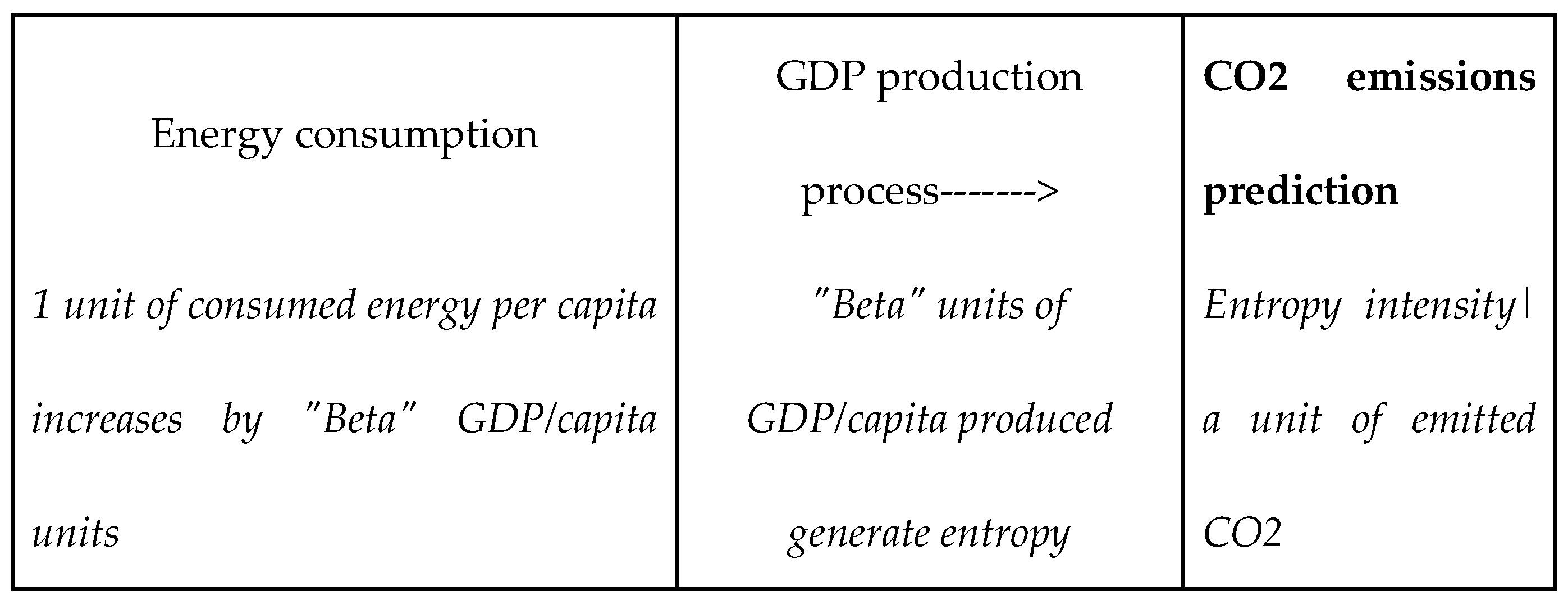
In the previous Section, we have defined the essence of the connection between production, entropy and CO2 emissions. Before presenting the outputs, let us yet explore a few recent works linking entropy and CO2 emissions. More recently, some authors explored close relationships between entropy and CO2 emissions. Moser (et al.) [73] proposed an entropy-based approach to assess the sustainability of production systems, considering both resource depletion and waste generation, including CO2 emissions. Warr et al. [74] revisited the connection between entropy, resource depletion, and economic growth, highlighting the role of CO2 emissions in increasing the entropy of the environment. Feng, C. and co-authors [75] investigated the relationship between entropy and CO2 emissions in China's industrial sectors, using a panel data analysis and entropy measures based on energy consumption. Qin, Q., and co-authors [76] examined the relationship between entropy, CO2 emissions, and economic growth in China, using a panel quantile regression approach to capture potential non-linearities and heterogeneity across regions. Korhonen and co-authors [77] focused on the chemical manufacturing industry, quantifying the relationship between energy consumption, CO2 emissions, and entropy metrics to identify opportunities for improving energy efficiency and reducing emissions. Casazza and co-authors [78] explored the use of entropy as a measure of circularity in economic systems, highlighting the connection between resource depletion, waste generation, and CO2 emissions in a circular economy context. These recent works demonstrate the ongoing research interest in understanding the thermodynamic foundations of economic production processes, particularly the connection between entropy and environmental impacts, such as CO2 emissions. The studies employ various methodologies, including panel data analysis, quantile regressions, and industry-specific case studies, to investigate this relationship across different scales and contexts. All these works use the Gaussian Gibbs-Shannon entropy which, as presented above, is limited to ergodic systems, thus less complex. Once again, the present work applies entropy based on the power law distribution more suited to dynamic systems, such as those related to economic production. Given the introductory information above, let us now return to the results. Using cross-section data in Table 2, we carried out a linear regression of entropy values on the CO2 emissions per head to capture average relationships between both variables. The estimated parameter “beta” amounts to 18.3 with a t-student equal to 11.49 suggesting a high significance of the estimate. This suggests that one can predict the CO2 emissions based on this estimate for the average case of this set of 10 countries. Thus, multiplying the above parameter estimate of 18.3 by a unit of entropy provides to the predicted value of CO2 emissions for each of the 10 countries. Nevertheless, this measure presents serious limitations if we need to predict with accuracy the emissions of each country. The last column of Table 2 proposes the factor of entropy intensity per a unit of CO2 emission per capita. With this factor, one can predict the CO2 emissions if and only if we have some knowledge on entropy emitted over a given time\space scale. Entropy values represent by definition a long run equilibrium of the system. This is a great advantage of the proposed methodology based on such a parameter emerging from long-run equilibrium. This a good starting point to perform reliable predictions. The next figure summarizes the relationships between energy consumption, GDP production, entropy generation and CO2 emissions. As said above it becomes possible to estimate or predict the level of CO2 emissions from the quantity of energy consumed and the estimate of the Entropy intensity per a unit of emitted CO2.
Figure 1.
Link between energy consumption and CO2 emissions through an economic production process.
However, the rule of the thumb is to interpret this value with caution since there could be other factors influencing both variables or a third variable influencing both entropy and CO2 emissions per GDP. For instance, the type of energy sources used in a country can influence both entropy and CO2 emissions per GDP. Countries that rely heavily on fossil fuels for energy production tend to have higher CO2 emissions per GDP, while the use of renewable energy sources may lead to lower emissions. The energy mix can also impact entropy levels due to the varying levels of complexity and disorder associated with different energy production processes.
3.2. Limitations of the Study and Prospective Research Area
Finally, the results in Table 1 go through another aspect of the problem posed by analyzing the complexity of the GDP-energy relationship using the power law related principle of maximum entropy. The model extends the analysis by attempting to evaluate the degrees of complexity (and/or organization) of the GDP formation process under the effect of energy stimuli. We considered that this complexity could be measured by the optimal amounts of entropy necessary to draw this system towards equilibrium [48] while consuming energy to generate economic commodities. Next, building on recent works, we extended the analysis and applied the non-extensive maximum entropy which outputs are presented in Table 1. Since this form of entropy generalizes that of Gibbs-Shannon and better suits to non-ergodic systems, of which economy dynamics, the obtained results should be more accurate. The last interesting issue, being the purpose of this study, concerns the prediction of carbon emissions based on the entropy produced during the process of economic production using energy. This point has just been initiated here and the quantitative statistical link between entropy and CO2 emissions has been found in this research, based on outputs in Table 2. Nevertheless, we invite interested researchers to possibly explore the proposed methodology in greater depth taking into account the following limitations. When computing CO2 emissions based on entropy values, there are several potential limitations and considerations that should be kept in mind. Data quality and availability: the accuracy of the computed CO2 emissions depends on the quality and completeness of the entropy and CO2 emissions data. Inconsistencies, measurement errors, or missing data points can introduce biases or errors in the analysis. The next limitations may result from omitted variable bias. As said earlier, the relationship between entropy and CO2 emissions may be influenced by other factors not accounted for in the regression model. Omitting relevant variables, such as economic indicators, energy mix, or technological progress, can lead to biased estimates of the entropy-CO2 emissions relationship. Fortunately enough, the input energy, as said earlier, remains besides the human capital, one of the most influential variable of the economic production. The second issue may concern endogeneity and reverse causality. The direction of causality between entropy and CO2 emissions may not be clear-cut. While entropy could influence CO2 emissions, CO2 emissions or other environmental factors could also contribute to changes in entropy levels. Failing to account for potential endogeneity or reverse causality can lead to biased and inconsistent estimates. As alluded to before about the entropy curve, non-linear and non-monotonic relationships may exist between entropy and CO2 emissions. In our case, the assumption of a monotonic relationship between entropy and CO2 emissions may lead to an oversimplification. The next main issue may concern temporal dynamics. In fact, the relationship between entropy and CO2 emissions may evolve over time due to changes in policies, technologies, or economic conditions. A static regression model may fail to capture these dynamic relationships accurately. The last limitation concerns uncertainty and sensitivity of the solution. In fact, the computed CO2 emissions based on entropy values may be sensitive to the chosen regression model, estimation methods, and assumptions. Conducting sensitivity analyses and quantifying the uncertainty associated with the estimates is essential for robust interpretations.
Fortunately enough, the use of a generalized entropy model (Tsallis entropy) as the one defined through the equations 1-3 is theoretically well fitting to the analyzed complex system of economic productiob while requiring the minimum of assumptions.
4. Concluding Remarks
The application of entropy concepts to analyze environmental impacts, particularly carbon dioxide (CO2) emissions, in economic production processes may offer a novel and insightful perspective. By quantifying the disorder and complexity associated with these processes, the entropic metric provides a holistic approach to understanding the intricate interplay between economic activities and their environmental consequences. The holistic nature of entropy qualitatively addresses the weaknesses presented by the other metrics presented in the first section of this paper. The results of this study highlight globally the positive correlation between entropy and CO2 emissions per unit of GDP, suggesting that as production processes become more complex and less organized, they tend to generate higher levels of CO2 emissions relative to their economic output. This finding underscores the importance of considering not only the economic efficiency but also the entropic efficiency of production systems. While the entropic metric does not directly measure CO2 emissions, it may capture the underlying factors that contribute to the generation of emissions, such as energy consumption - the targeted variable in our study, resource depletion, and waste production. By focusing on these fundamental drivers, the entropic approach may provide a comprehensive framework for evaluating the sustainability of economic activities. The originality of this study is the use of the power law based (Tsallis) entropy designed to handle non-ergodic systems. As already alluded to in this paper, in such systems, the entropy of the whole is not necessarily equal to the sum of the entropies of its parts. This property makes power law-based entropies more suitable for analyzing complex systems with long-range interactions or correlations, which are common in economic and environmental processes.
Thanks to this work, we have introduced and analyzed the role of energy as a central factor of economic production. This strong hypothesis is at the core of the presented model defining the relationships between the triad of energy, economic production and CO2 emissions.
Nevertheless, it is important to recognize the relative limitations of this study, including potential omitted variable biases, and plausible uncertainties associated with entropy computation and CO2 emissions data. Future research could explore more advanced techniques for quantifying entropy, incorporate additional control variables, and investigate the temporal dynamics of the entropy-emissions relationship. Despite these limitations, the entropic metric offers a promising avenue for policymakers, industry leaders, and researchers to assess the environmental impacts of economic activities from a novel perspective based on a holistic methodology extended to non-ergodic processes. By integrating entropic considerations into decision-making processes, stakeholders can identify opportunities for reducing CO2 emissions while maintaining economic productivity. According to authors, this new metrics should represent a step towards a more comprehensive understanding of the intricate interplay between economic activities and environmental impacts, paving the way for more informed and responsible decision-making in the pursuit of a sustainable future.
References
- IPCC. Guidelines for National Greenhouse Gas Inventories. 2006.
- Oda and al., et. The Open-source Data Inventory for Anthropogenic CO2, version 2016 (ODIAC2016). Earth System Science Data. 2018.
- Peters and Hertwich. ISO 14040 and 14044. Carbon Footprint of Nations. Environmental Science & Technology. 2009.
- Davis and Caldeira. Consumption-based accounting of CO2 emissions. PNAS. 2010.
- Wiedmann & Minx. A Definition of 'Carbon Footprint'. Ecological Economics Research Trends. 2008.
- Marland and al., et. Accounting for uncertainty in CO2 emissions. Nature Geoscience. 2009.
- Métayer and al., et. Uncertainty in spatially explicit CO2 emission models. International Journal of Greenhouse Gas Control. 2012.
- Nordhaus. The DICE model: Background and structure of a dynamic integrated climate-economy model of the economics of global warming. 2013.
- Rolnick and al., et. Tackling Climate Change with Machine Learning. arXiv:1906.05433. 2019.
- Wiedmann, T. and Minx, J. A Definition of Carbon Footprint. Ecological Economics Research Trends. 2008, Vol. 1, pp. 1-11.
- Majeau-Bettez, G. , Hawkins TR, TR and Strømman, AH. Life cycle environmental assessment of lithium-ion and nickel metal hydride batteries for plug-in hybrid and battery electric vehicles. Environ Sci Technol. may 15, 2011, pp. 4548-54.
- Lenzen, M. Errors in Conventional and Input-Output—based Life—Cycle Inventories. Journal of Industrial Ecology. 4, 2000, pp. 127-148.
- Su, B.; Ang, B. Input–output analysis of CO2 emissions embodied in trade: The effects of spatial aggregation. Ecol. Econ. 2010, 70, 10–18. [Google Scholar] [CrossRef]
- Peters, G.P.; Hertwich, E.G. Post-Kyoto greenhouse gas inventories: production versus consumption. Clim. Chang. 2007, 86, 51–66. [Google Scholar] [CrossRef]
- Caldeira, Dawis. Consumption-based accounting of CO2 emissions. 107, Mars 8, 2010, Vol. 12, pp. 5687-5692.
- Ang,, B. W. Is the energy intensity a less useful indicator than the carbon factor in the study of climate change? Energy Policy. 27, 1999, Vol. 15, pp. 943-946.
- Rypdal,, Kristin and Wilfried, Winiwarter. Uncertainties in greenhouse gas emission inventories—evaluation, comparability and implications. Environmental Science & Policy. 4, 2001, Vols. 2-3, pp. 107-116.
- Acquaye, A.A.; Wiedmann, T.; Feng, K.; Crawford, R.H.; Barrett, J.; Kuylenstierna, J.; Duffy, A.P.; Koh, S.C.L.; McQueen-Mason, S. Identification of ‘Carbon Hot-Spots’ and Quantification of GHG Intensities in the Biodiesel Supply Chain Using Hybrid LCA and Structural Path Analysis. Environ. Sci. Technol. 2011, 45, 2471–2478. [Google Scholar] [CrossRef]
- Kevin, R. Gurney,, et al. High Resolution Fossil Fuel Combustion CO2 Emission Fluxes for the United States 2009. Environmental Science & Technology. 43, 2009.
- Guan, and Dabo, et al.. The gigatonne gap in China’s carbon dioxide inventories. Nature Climate Change. 2, 2012, Vol. 9, pp. 672-675.
- Moss,, Richard H, et al.
- Tong,, C. J., et al. Microstructure characterization of Al x CoCrCuFeNi high-entropy alloy system with multiprincipal elements. Metallurgical and Materials Transactions A,. 2005, Vol. 3, 36,, pp. 881-893.
- Georgescu-Roegen. The Entropy Law and the Economic Process. 1971.
- Ayres, R.U.; Warr, B. The Economic Growth Engine; Edward Elgar Publishing: Cheltenham Glos, United Kingdom, 2009. [Google Scholar]
- Prigogine, I.; Van Rysselberghe, P. Introduction to Thermodynamics of Irreversible Processes. J. Electrochem. Soc. 1963, 110, 97C. [Google Scholar] [CrossRef]
- Faber, M. , Niemes, H. and Stephan, G. Entropy, Environment, and Resources. 1987.
- Kümmel, R. The Second Law of Economics; Stern. 2011.
- The Role of Entropy in the Development of Economics. Jakimowicz, Aleksander. 4, 2020, Entropy, Vol. 22, p. 452.
- IPCC. Climate Change 2021: The Physical Science Basis. 2021.
- Energy, aesthetics and knowledge in complex economic systems. Foster, John. 1, 2011, Journal of Economic Behavior & Organization, Vol. Volume 80, pp. 88-100.
- A Brief History of Energy Use in Human Societies. In: Revisiting the Energy-Development Link. SpringerBriefs in Economics. Springer, Cham. Bithas, K. and Kalimeris, P. 2016, Springer International Publishing.
- Blaug, Mark. Economic Theory in Retrospect (4th ed.). Cambridge : Cambridge University Press, 1985. ISBN 978-0521316446.
- Stigler, J. George. Essays in the History of Economics.. Chicago : University of Chicago Press., 1965.
- A Contribution to the Theory of Economic Growth. Solow, Robert. 56), Quarterly Journal of Economics, pp. 65-94. 19 February.
- Robert, M. Solow's Neoclassical Growth Model: An Influential Contribution to Economics. Edward C., C. Prescott. No. 1, s.l. : The Scandinavian Journal of Economics, Mar., 1988, Vol. Vol. 90, pp. 7-12.
- ENDOCENOUS TECHNOLOGICAL CHANGE. Romer, M. ENDOCENOUS TECHNOLOGICAL CHANGE. Romer, M. Paul. Massachusetts : NATIONAL BUREAU OF ECONOMIC RESEARCH, 1989. Working Paper No. 3210.
- On the mechanics of economic development. Lucas, Lucas and Robert, E. s.l. : Journal of Monetary Economics, 1988, Vol. 22, pp. 3-42.
- Government Spending in a Simple Model of Endogenous Growth. Barro, RJ. Government Spending in a Simple Model of Endogenous Growth. Barro, RJ. 1990, Journal of Political Economy, Vol. 98, pp. 103-125.
- Rodrik, D. . One Economics Many Recipes: Globalization, Institutions, and Economic Growth. Princeton : Princeton University Press, 2007.
- Okrasa, W. , & Rozkrut, D.. The Time Use Data-based Measures of the Wellbeing Effect of Community Development: An Evaluative Approach. imsva91-ctp.trendmicro.com. [Online] Polish Institute of Statistics, 2018. https://imsva91-ctp.trendmicro.com:443/wis/clicktime/v1/query?url=https%3a%2f%2fnces.ed.gov%2fFCSM%2f2018%5fResear.
- Cierpial-Wolan, M. . The modelling of cross-border aspects of territorial development. Rzeszow : University of Rzeszow Publishing House, 2022.
- The relationship between energy consumption and economic growth: Evidence from non-Granger causality test. Faisal, Faisal, Turgut, Tursoy and Ercantan, Ozlem. s.l. : Procedia Computer Science, 2017, Vol. 120, pp. 671-675. ISSN 1877-0509.
- Economic Growth with Energy. Alam, M. Economic Growth with Energy. Alam, M. Shahid. Boston : MPRA Paper, Northeaster University, 2006.
- Causal Relationships between Energy Consumption and Economic Growth. Zhang, Zhixin and Ren, Xin. s.l. : Energy Procedia, 2011, Vol. 5, pp. 2065-2071. ISSN 1876-6102.
- The triangular relationship between energy consumption, trade openness and economic growth: new empirical evidence. Osei-Assibey, Bonsu and Wang, M. Y. 1, s.l. : Cogent Economics & Finance, 2022, Vol. 10. Article 2140520.
- Relationship between Energy Consumption and Economic Growth in European Countries: Evidence from Dynamic Panel Data Analysis. Topolewski, Łukasz. 12, s.l. : MDPI, 2021, Energies, Vol. 14. 3565.
- ENERGY–GDP RELATIONSHIP: A CAUSAL ANALYSIS FOR THE FIVE COUNTRIES OF SOUTH ASIA. ASGHAR, Zahid. 1, s.l. : Applied Econometrics and International Development, 2008, Vol. 8.
- A survey of literature on energy consumption and economic growth. Sebabi, Geoffrey Mutumba, et al. s.l. : Energy Reports, 2021, Vol. 7, pp. 9150-9239.
- Grossman, G. and Krueger, A. Economic growth and the environment. Quarterly Journal of Economics. 1995, Vol. 110, pp. 353–77.
- Soumyananda, Dinda. Environmental Kuznets Curve Hypothesis: A Survey. Ecological Economics. 2004, 49, pp. 431–455.
- Stern, D.I. The environmental Kuznets curve after 25 years. J. Bioeconomics 2017, 19, 7–28. [Google Scholar] [CrossRef]
- Ang, J. B. CO2 emissions, energy consumption, and output in France. [Online] 2007.
- Shahbaz, M.; Hye, Q.M.A.; Tiwari, A.K.; Leitão, N.C. Economic growth, energy consumption, financial development, international trade and CO2 emissions in Indonesia. Renew. Sustain. Energy Rev. 2013, 25, 109–121. [Google Scholar] [CrossRef]
- Gabaix, X. The Laws of Power in Economics and Finance. Washington : BER, 2008.
- Aggregate Fluctuations from Independent Sectoral Shocks: Self-organized Criticality in a Model of Production and Inventory Dynamics. Bak, et al. 1, s.l. : Ricerche Economiche, 1993, Vol. 47, pp. 3–30.
- Miziołek, T.; Filip, D. Market Concentration in the Polish Investment Fund Industry. Gospod. Nar. 2019, 300, 53–78. [Google Scholar] [CrossRef]
- Bwanakare, S. Non-Extensive Entropy Econometrics for Low Frequency Series: National Accounts-Based Inverse Problems. Warsaw : De Gruyter Open Poland, 2018.
- Jakimowicz, A. The Material Entropy and the Fourth Law of Thermodynamics in the Evaluation of Energy Technologies of the Future. Energies 2023, 16, 3861. [Google Scholar] [CrossRef]
- Taleb, N.N. The Black Swan; Random House: New York, NY, USA, 2007; ISBN 978-1-4000-6351-2. [Google Scholar]
- Power Laws in Economics: An Introduction. Gabaix, Xavier. 1, s.l. : Journal of Economic Perspectives, 2016 (February), Vol. 30, pp. 185–206.
- Judge, George G., Miller, Douglas and Golan, Amos. Maximum Entropy Econometrics : Robust Estimation with Limited Data. s.l. : Chichester [England]: Wiley., 1996.
- Tsallis,, Constantino. Introduction to Nonextensive Statistical Mechanics, Approaching a Complex World. [ed.] Springer. NewYork : s.n., 09. 10.1007/978-0-387-85359-8. 20 January.
- A mathematical theory of evolution based on the conclusions of Dr. JC Willis FRS . Yule, G. U. no. A mathematical theory of evolution based on the conclusions of Dr. JC Willis FRS. Yule, G. U. no. 402–410, London : Royal Soc., , 1925, Phil. Trans.B, Vol. 213, pp. 21-87. 1 January.
- A Model of Income Distribution. Champernowne, D. G. A Model of Income Distribution. Champernowne, D. G. 1, s.l. : The Economic Journal, 1953, Vol. 63, pp. 318–351.
- On a class of skew distribution functions. Simon, H. A. On a class of skew distribution functions. Simon, H. A.. 3-4, s.l. : Biometrika, 1955, Vol. 42, pp. 425-440.
- Limit theorems for stochastic growth models. II. Kesten, H. Limit theorems for stochastic growth models. II. Kesten, H. 3, s.l. : Advances in Applied Probability, 1972, Vol. 4, pp. 393-428.
- Jessen, Anders Hedegaard and Mikosch, Thomas. Regularly Varying Functions. s.l. : Publications de l'Institut Mathématique, 2006. Vol. 80(94), 100, pp. 171-192.
- Bottazzi, G.; Cefis, E.; Dosi, G.; Secchi, A. Invariances and Diversities in the Patterns of Industrial Evolution: Some Evidence from Italian Manufacturing Industries. Small Bus. Econ. 2006, 29, 137–159. [Google Scholar] [CrossRef]
- Champernowne, D.G. A Model of Income Distribution. Econ. J. 1953, 63, 318. [Google Scholar] [CrossRef]
- Stanley, (et al.) and Eugene, H. Power Law Scaling for a System of Interacting Units with Complex Internal Structure,. PHYS I CAL RE V I EW LETTERS,. , 1998. 16 February.
- Eurostat. Eurostat. [Online] EU, 2023. https://ec.europa.eu/eurostat/databrowser/view/ten00122/default/table?lang=en.
- Energy Efficiency Forecast as an Inverse Stochastic Problem: A Cross-Entropy Econometrics Approach. Bwanakare, S. s.l. Energy Efficiency Forecast as an Inverse Stochastic Problem: A Cross-Entropy Econometrics Approach. Bwanakare, S. s.l. : MDPI, 2023, Energies, Vol. 16.
- Moser, S. , Kainz, C. and Loy, C. Entropy as a measure for assessing the sustainability of production systems. Sustainability. 13, 2021, Vol. 4, 1761.
- Warr, B. and Ayres, R. U. Entropy, resources, and economic growth. Ecological Economics. 193, 2022, Vol. 107295.
- Feng, C. , et al. Exploring the entropy-emission nexus: Evidence from China's industrial sectors. Energy Economics. 109, 2022, Vol. 105992.
- Qin, Q. , Liu, Y. Energy Reports. 2021, 4769–4778. [Google Scholar]
- Korhonen, J. and Snäkin, J. P. Quantifying the relationship between energy consumption, CO2 emissions, and entropy metrics for chemical manufacturing processes. Journal of Cleaner Production,. 246, 2020, Vol. 119005.
- Casazza, M. and Manfren, M. The role of entropy in assessing the circularity of economic systems. Entropy. 24, 2022, Vol. 5, 600.
- Quesnay, Francois. Tableau Economique. London : MacMilian and Co and New York, 1894.
- Razzaqi, S.; Bilquees, F.; Sherbaz, S. .. Dynamic Relationship Between Energy and Economic Growth: Evidence from D8 Countries. Pak. Dev. Rev. 2022, 50, 437–458. [Google Scholar] [CrossRef]
- KELSEY, JACK. How much do we know about the development impacts of energy infrastructure? Published on. Sustainable Energy for All,. [Online] MARCH 29, 2022. https://blogs.worldbank.org/energy/how-much-do-we-know-about-development-impacts-energy-infrastructure.
- Magazzino, C.; Schneider, N. The Causal Relationship between Primary Energy Consumption and Economic Growth in Israel: A Multivariate Approach. Int. Rev. Environ. Resour. Econ. 2020, 14, 417–491. [Google Scholar] [CrossRef]
- Gell-Mann, M. and Tsallis, C. Nonextensive Entropy, Interdisciplinary Applications. New York, NY, USA : Oxford University Press, 2004.
- Nordhaus. The DICE model: Background and structure of a dynamic integrated climate-economy model of the economics of global warming. 2013.
- Stern, D. I. The role of energy in economic growth. Annals of the New York Academy of Sciences. 2011.
- Stern, D.I. The environmental Kuznets curve after 25 years. J. Bioeconomics 2017, 19, 7–28. [Google Scholar] [CrossRef]
- Soytas, U.; Sari, R. Energy consumption, economic growth, and carbon emissions: Challenges faced by an EU candidate member. 68, 1667. [Google Scholar] [CrossRef]
- Halicioglu and Ferda. An econometric study of CO2 emissions, energy consumption, income and foreign trade in Turkey. Energy Policy. 37, 09, Vol. 3, pp. 1156-1164. 20 March.
- A Brief History of Energy Use in Human Societies. In: Revisiting the Energy-Development Link. Springer Briefs in Economics. Springer, Cham. Bithas, K. and Kalimeris, P. 2016, Springer International Publishing.

Table 1.
Entropy-based model outputs for 10 EU countries. Response variable: GDP/per capita, Regressor: consumed energy per capita.
Table 1.
Entropy-based model outputs for 10 EU countries. Response variable: GDP/per capita, Regressor: consumed energy per capita.
| Country | Estimates | Model R^2 _equivalent |
Optimal entropy values |
|
| Beta | constant | |||
| Denmark | 5.443 | 1.335 | 0.876 | 0.435 |
| Belgium | 3.836 | 1 | 0.918 | 0.45 |
| Germany | 4.867 | 1.089 | 0.937 | 0.488 |
| Netherlands | 4.279 | 1.603 | 0.334 | 0.496 |
| Czechia | 2.963 | 0.872 | 0.955 | 0.52 |
| Ireland | 3.731 | 2.417 | 0.565 | 0.525 |
| France | 5.037 | 0.71 | 0.951 | 0.528 |
| Estonia | 2.204 | 0.832 | 0.943 | 0.552 |
| Poland | 3.065 | 0.742 | 0.982 | 0.552 |
| Bulgaria | 2.01 | 0.575 | 0.982 | 0.555 |
Source: own calculations.
Table 2.
Entropy intensity per unit of CO2 as a CO2 predictor factor.
| countries | CO2\capita | Entropy intensity per a unit of CO2 per capita |
| Belgium | 9.949232 | 0.04523 |
| Bulgaria | 6.700354 | 0.082831 |
| Czechia | 11.26775 | 0.046149 |
| Denmark | 7.73826 | 0.056214 |
| Germany | 9.846759 | 0.049559 |
| Estonia | 14.65488 | 0.037667 |
| Ireland | 9.064644 | 0.057917 |
| France | 5.809483 | 0.090886 |
| Netherlands | 10.43629 | 0.047526 |
| Poland | 8.303462 | 0.066478 |
Disclaimer/Publisher’s Note: The statements, opinions and data contained in all publications are solely those of the individual author(s) and contributor(s) and not of MDPI and/or the editor(s). MDPI and/or the editor(s) disclaim responsibility for any injury to people or property resulting from any ideas, methods, instructions or products referred to in the content. |
© 2024 by the authors. Licensee MDPI, Basel, Switzerland. This article is an open access article distributed under the terms and conditions of the Creative Commons Attribution (CC BY) license (https://creativecommons.org/licenses/by/4.0/).
Copyright: This open access article is published under a Creative Commons CC BY 4.0 license, which permit the free download, distribution, and reuse, provided that the author and preprint are cited in any reuse.


