
Submitted:
21 November 2024
Posted:
22 November 2024
You are already at the latest version
Abstract
As Unmanned Aerial Vehicles (UAVs) are becoming crucial in modern warfare, research on autonomous path planning is becoming increasingly important. The conflicting nature of the optimization objectives characterizes path planning as a multi-objective optimization problem. Current research has predominantly focused on developing new optimization algorithms. Although being able to find the mathematical optimum is important, one also needs to ensure this optimum aligns with the decision-maker's (DM's) most preferred solution (MPS). In particular, to align these, one needs to handle the DM's preferences on the relative importance of each optimization objective. This paper provides a comprehensive overview of all preference handling techniques employed in the military UAV path planning literature over the last two decades. It shows that most of the literature handles preferences by the overly simplistic method of scalarization via weighted sum. Additionally, the current literature neglects to evaluate the performance (e.g. cognitive validity and modeling accuracy) of the chosen preference handling technique. To aid future researchers handle preferences, we discuss each employed preference handling technique, their implications, advantages, and disadvantages in detail. Finally, we identify several directions for future research, mainly related to aligning the mathematical optimum to the MPS.
Keywords:
UAV
; preference handling
; multi-objective optimization
; path planning
; radar
; mission planning
1. Introduction
The first documented military use of Unmanned Aerial Vehicles (UAVs) occurred in 1849 when the Austrian forces deployed around 200 hot-air balloons to bomb Venice [1]. Half a century later, in the Great War, the first pilotless aircraft was developed [2]. Although the balloons had little effect, and the aircraft were never used operationally, both showed a glimpse of the future of warfare. It was in the Vietnam war when reconnaissance UAVs were deployed on a large scale for the first time [2], flying over 3000 missions [3]. Later, during the battle of the Beka’a valley in 1982, decoy UAVs helped the Israeli air force win a decisive victory, destroying 17 out of 19 Syrian SA-6 air defence systems in ten minutes [3,4]. As a response, the Syrians sent out a large number of MiG jet fighters. However, with the help of a reconnaissance drone providing live video imagery of the take off of the jet fighters, Israel was perfectly prepared for the attack. At the end of the war, Syria lost 85 MiGs, whilst failing to destroy a single Israeli aircraft. As a result of the massive success of the operation the Israeli Air Force increased their UAV force substantially [3]. Nowadays, UAVs have become such a crucial asset on the battlefield, that the Russia-Ukraine war has been named the first drone war. Small inexpensive radio-controlled drones are being used on a wide scale to destroy millions of dollars of tanks and artillery systems [5]. One major threat against these radio-controlled drones is the use of Electronic Warfare (EW) systems to jam the drones’ radio frequencies or to trace the signal back to the drone operator. In fact, Russia’s EW systems are causing Ukraine to lose approximately drones per month [6]. In response, Ukraine and Russia are investing heavily in Artificial Intelligence guided drones [5], for they have no radio frequency to jam nor an operator to trace the signal back to. Although the technology required still needs to be developed further, many believe that autonomous drones will be at the heart of future drone warfare [5,7].
One key feature for UAVs to operate without direct human control is autonomous navigation and flight. It involves the formulation of a global pre-mission flight path as well as local optimization based on real-time data during flight. In military applications, missions are meticulously planned, making pre-mission flight path planning especially crucial. Therefore the scope of this paper is on pre-mission path planning and for the remainder of the paper, the term "path planning" specifically refers to pre-mission path planning. Path planning can be defined as finding the optimal feasible route from point A to point B (possibly involving more points). A feasible route is one that meets the constraints posed by the UAV’s flight dynamics. Besides feasibility, it is important for a route to achieve certain goals. For example, it needs to be short, have minimal fuel consumption, and in a military context, be safe from hostile actors. Mathematically, these goals are quantified as optimization objectives and they can be conflicting. Conflicting objectives cannot be optimized simultaneously and thus trade-offs need to be made. For instance, a possible detour to evade a radar system will decrease the probability of detection, but increase route length. Similarly, flying fast will reduce the time in air but increase fuel consumption. Note that although the scope of this review is on military UAV path planning, civilian UAV path planning also has conflicting objectives (e.g. speed and fuel-efficiency). Therefore, the discussion below, especially the detailed discussion on different preference handling methods, is also relevant for civilian UAVs. The presence of these conflicting optimization objectives characterizes the UAV route planning problem as a multi-objective optimization (MOO) problem described by Equation 1. For illustrative purposes we have avoided unnecessary mathematical rigour and described the problem loosely.
The MOO problem loosely described by Equation (1) consists of five components. For each decision variable (1) x, a set of kobjectives (2) () is computed. In the context of route planning, the decision variable x represents a route, which is a time-dependent function over 3-dimensional spatial coordinates. Additionally, it includes parameters like the velocity, acceleration, and yaw angle. Even though is continuous, many path planning methods work on a discretized version of the problem. The k objective functions measure the performance of each route based on a certain metric. For instance, in the simplified example visualized in Figure 1, the objectives () of minimizing route length and danger are included. Moreover, each solution (i.e. route) must satisfy the flight constraints (3) imposed by the UAV’s flight dynamics to be included in the feasible set . Based on these ingredients, an optimization algorithm (4) searches for the optimal route. However, in multi-objective optimization, optimality is less straightforward than in single-objective optimization, which is why the quotation marks in "minimize" are included. Rather than dealing with scalar objective values, multi-dimensional objective vectors are considered, meaning the minimum is not simply the lowest objective value. Consequently, a different notion of optimality is needed. Pareto optimality defines a solution x as optimal when none of its objectives can be improved without deteriorating the performance of another objective [8]. If such an improvement was possible, route would be said to dominate route x. Of course, no rational decision-maker (DM) would ever prefer a dominated solution over the solution that dominates it. This is exactly what Pareto optimality captures; all non-dominated solutions are Pareto optimal. This (possibly infinite) set of optimal solutions is called the Pareto Front. Mathematically speaking, all routes on the Pareto Front are equally good. However, a DM will prefer some routes over others. For example, in the simplified Figure 1a, two optimal 2-dimensional routes are visualized: the short but dangerous route , and the long but safe route . As they are both on the Pareto Front (see Figure 1b), neither route nor route is mathematically better than the other. Yet, depending on the mission scenario a DM might prefer over or vice versa. In particular, the relative importance of each objective can vary per mission. For instance, a high-risk, time critical, rescue mission will accept higher danger levels than a simple transport mission. Moreover, losing a small quadrotor UAV is less important than losing a large expensive fixed wing UAV. Essentially, the DM’s preferences determine which solution on the Pareto front is the DM’s most preferred solution (MPS). Preference handling (5) integrates the DM’s subjective preferences into the optimization model to align the mathematical optimum to the DM’s subjective optimum (i.e. the MPS). This is crucial, as the goal of the path planning problem is not to arrive at a mathematical optimum but rather to help the DMs arrive at their MPS. Commonly, a scalar composite objective function is defined that aggregates the individual objectives. The specific aggregation function h differs per method (e.g. product in Section 4.1.1 and weighted-sum in Section 4.2.1). Many other methods exist, each having their own advantages and disadvantages.
Over the past decades, UAV path planning has been an active research field. Many papers have proposed novel approaches to model one (or multiple) of the five aforementioned components. So far, the literature has predominantly focused on developing new optimization algorithms. This trend is also evident in existing review papers. Indeed, as shown in Table 1, every survey has extensively covered the optimization algorithms (component (4)) proposed by the literature. Component (1), how to model routes, has been covered by both Aggarwal & Kumar [9] and Jones et al. [10]. They proposed a classification based on Cell Decomposition approaches, Roadmap approaches, and Artificial Potential Field approaches. As most of the approaches make a discrete approximation of the continuous 3D space by a grid or a graph, the planned route has a lot of sharp turns. Therefore, to ensure the route satisfies the flight constraints imposed by the UAV, the route needs to be smoothed. An overview of trajectory smoothing techniques is provided by Ravankar et al. [11]. The remaining three key components, the modeling of the optimization objectives (2), constraints (3) and preference handling (5), on the other hand, have largely been neglected. Most surveys fail to mention the existence of the optimization objectives and the flight constraints. The surveys that do, Song et al. [12] and Saadi et al. [13], only minimally describe the presence of certain objectives and constraints but do not cover the different modeling choices nor their implications. Preference handling (component (5)) is touched upon by Song et al. [12], yet they only briefly mention the weighted sum method as a potential modeling choice without going into detail. Although surveys on objective and constraint modeling would be useful, this review aims to address the lack of focus on preference handling. As mentioned before, preference handling aims to align the DM’s subjective optimum with the mathematical optimum of the optimization model. Clearly, even if the optimization algorithm is perfect, it will never reach the MPS if preference handling is done incorrectly. Therefore, focusing on preference handling is of paramount importance. This review provides a comprehensive overview of preference handling in the military UAV path planning literature over the last twenty years. Both the methods and the implications arising from choosing these methods are discussed. By doing so, we aim to answer the following two research questions (RQs):
- RQ1: What preference handling techniques have been used in the military UAV path planning literature?
- RQ2: For each of the identified methods: What are the advantages and disadvantages of using these methods?
By answering RQ1, we aim to provide an overview of the preference handling methods used in the military UAV route planning literature. This overview provides insight into the state of the art, thereby identifying gaps in the research literature. In particular, we aim to identify the extent to which DMs have been included in the literature. By answering RQ2, we aim to provide future researchers with an overview of the advantages and disadvantages of the employed preference handling methods. This critical discussion intends to provide future researchers the necessary tools to determine which preference handling method to use. In particular, this aims to help researchers ensure that their problem modeling aligns the mathematical optimum to the DM’s MPS.
The remainder of this paper is organized as follows. Section 2 describes the research methodology. In particular, the process of selecting the papers included in this review are described. In Section 3, to answer RQ1, we provide a comprehensive overview of the different preference handling techniques employed in the literature. Furthermore, we investigate the extent to which DMs have been included in the performance evaluation of the proposed methods. Next, in Section 4, to answer RQ2, a critical discussion of the advantages and disadvantages of each preference handling method employed in the literature is provided. Finally, Section 5 concludes the paper and identifies directions for future research.
2. Methodology
This scoping review is largely based on the guidelines for PRISMA Scoping Reviews by Tricco et al. [15]. The review’s scope focuses on UAV path planning in hostile environments. In particular, the focus lies on environments with hostile actors such as enemy radars and anti-air defences. To identify potentially relevant papers, the databases of the Netherlands Defence Academy (NLDA), the American Naval Postgraduate School (NPS), and the American Institute of Aeronautics and Astronautics (AIAA) were searched from 2003-2024. The NLDA and NPS libraries consist of a collection of multiple databases. For example, the NLDA library yields access to IEEE, ProQuest, Springer, and many more. The NPS library yields access to over 300 databases. Finally, AIAA is the world’s largest aerospace technical society with over technical articles, including both military and civilian applications. The focus on hostile environments corresponds well to the military setting covered by the NPS and NLDA. Their extensive collection should cover most of the literature relevant to the review. The remaining gaps will be covered by the literature from AIAA, which includes a large set of technical aviation papers.
To search these databases the keywords need to cover the route planning aspect, as well as the hostile environment aspect. To include the route planning aspect, the following keywords are used: "Route planning" or "path planning". For the hostile environment, we identified that the literature predominantly includes radars or anti-air defence systems as hostile actors. Therefore, we include the combination of threat or hostile and specify it to a military setting by adding the keywords missile or radar. Note that we have chosen not to restrict our keyword search to UAV path planning per se. As path planning for manned systems shares a lot of similarities to path planning for unmanned systems, we have chosen to include both. However, even though we did not restrict ourselves to UAV path planning, no papers focusing on pre-mission path planning for manned systems were retrieved. The resulting keyword search which was last performed on 13-08-2024 is:
- ("Route planning" OR "Path planning") AND (hostile OR threat) AND (radar OR missile)
The keyword search resulted in a set of 848 papers, out of which 187 were duplicates. To filter this large set of papers to a representative and relevant set that can answer the proposed research questions, the procedure visualized in Figure 2 was performed. First, duplicates were removed. Secondly, for the remaining 661 papers, relevancy was judged based on the title and abstract. In this first check, 408 articles were removed. The reasons for removal were mainly because the papers were either not about flight path planning, or had no military application. Subsequently, from the 253 reports identified, 251 papers were retrieved. For these papers, the relevance was judged based on a full text read, and the eligibility criteria in Table 2 were used. The criterion of academic relevance was included to restrict the set of papers to a set representative of the general academic consensus. The general idea is that papers that are rarely cited, have not made an impact on the route planning research community. Note that by requiring papers to be cited at least once a year, new papers with few citations are still included in the paper selection. Next, papers that completely avoided threats or ignored them altogether were removed because in military missions it is rarely possible to completely avoid threats. Completely ignoring threats, on the other hand, simplifies the problem in such a way that it is irrelevant to actual practical applications. Similarly, by solely minimizing the distance or threat the multi-objective nature of the problem is neglected and is therefore irrelevant to this literature review. Papers that do not focus on flight route planning clearly fall out of the scope of the paper. Finally, papers where no details on the methods were reported or which only had minor changes to existing research were removed. The final set of papers included in this review consists of 76 studies that form a representative subset of military UAV route planning papers.
For each of these papers, we categorized the preference handling technique into four different classes based on the point at which the DM’s preferences were included. Furthermore, we extracted more detailed information on the preference handling technique. More particularly, the specific method used was documented for each paper. Based on this information, a general overview of the state of the art of preference handling in the military UAV path planning community was provided to answer RQ1. Additionally, to identify whether papers evaluated the practical usability of their methods, we extracted how the method was evaluated (e.g. was a subject matter expert used as DM). To answer RQ2, we explain each method in further detail. In particular, we describe the advantages and disadvantages of the modeling choices identified in the preference handling stage.
3. Preference Handling in the UAV Route Planning Literature
Based on the point in the optimization process at which the preferences of the DM are included, the multi-objective optimization (MOO) literature [17] uses four different categories of handling conflicting objectives (see Figure 3). The preferences of the DM decide which routes from the Pareto front are preferred over others. The preferences can be integrated either not at all (no preference method), before (a-priori), after (a-posterior), or progressively during the optimization process (interactive). For the military UAV route planning problem, the DM can be the drone operator, an intel officer, or anyone else who plans the route.
-
No-preference Preference HandlingFirstly, in no-preference methods, the DM is not involved in the process. Instead, a solution which is a neutral compromise between all objectives is identified. This method is commonly used when no DM is present and it usually constructs a scalar composite objective function .
-
a-priori Preference HandlingSecondly, in a-priori methods, a DM specifies their preference information before the optimization process is started. Most commonly, the preference information is used to construct a scalar composite objective function . This has the advantage that the problem is simplified into a single-objective optimization problem. As a result existing single-objective optimization algorithms can be used. The main limitation is that the DM has limited knowledge of the problem beforehand, which can result in inaccurate and misleading preferences [18,19]. Intuitively, asking the DM to specify their preferences before the optimization corresponds to asking them to select a point on the Pareto Front (e.g. by specifying objective weights) before knowing what the actual Pareto Front and its corresponding tradeoffs look like. Consequently, a set of preferences specified a-priori might lead to solution x, whereas the DM might have preferred y when presented with both options.
-
a-posterior Preference HandlingAlternatively, a-posterior methods can be used. These methods include the DM’s preferences after the optimization process. First, they approximate the Pareto Front and then allow the DM to choose a solution from said front. The main advantage is that the DM can elicit their preferences on the basis of the information provided by the Pareto Front. The DM has a better idea of the tradeoffs present in the problem and can thus make a better-informed choice. Furthermore, it can provide the DM with several alternatives rather than a single solution. The disadvantage of this class of methods is the large computational complexity of generating an entire set of Pareto optimal solutions [20]. Additionally, when the Pareto Front is high-dimensional, the large amount of information can cognitively overload and complicate the decision of the DM [18].
-
Interactive Preference HandlingFinally, interactive preference elicitation attempts to overcome the limitations of the a-priori and a-posterior classes by actively involving the DM in the optimization process. As opposed to the sequential views of a-priori and a-posterior methods, the optimization process is an iterative cycle. Optimization is alternated with preference elicitation to iteratively update a preference model of the DM and to quickly identify regions of the Pareto Front that are preferred. Undesired parts of the Pareto Front need not be generated, which saves computational resources. Instead, these resources can be spent on better approximating the preferred regions, improving their approximation quality [21]. Lastly, being embedded in the optimization process helps the DM build trust in the model and a better understanding of the problem, the tradeoffs involved, and the feasibility of their preferences [22,23,24]. One challenge of interactive methods is that the interaction needs to be explicit enough to build an expressive and informative model of the DM’s preferences whilst also being simple enough for the DM to not cognitively overload them.
Within the UAV route planning literature, there is a large focus on a-priori preference handling approaches. Indeed, Figure 4 (for the raw data see Table A1), shows that, despite its weaknesses, over 90% of the approaches use a-priori preference handling techniques. In fact, only two papers used a no-preference handling method, four used preference handling after optimization, and only one paper used interactive preference handling. The remaining 69 papers all used a-priori preference handling. One likely cause for this predominant focus on a-priori preference handling is that these methods simplify the problem to a single-objective optimization problem, thereby allowing the authors to use single-objective optimization techniques. Another cause might be that authors are not familiar with multi-objective optimization. This is substantiated by the fact that 70% of the papers use the simple intuitive weighted sum method (see Section 4.2.1), often a method that comes to mind first when dealing with multiple optimization objectives. Besides a methodological bias on a-priori preference handling techniques, many papers neglect the DM altogether. In particular, as shown in Figure 5, 50 papers (66%) simply assumed the preference information to be known. They did not experiment with different preferences, nor how a DM should arrive at them. On the other hand, 15 papers (20%) did provide some examples of different preference information, such as a different weight vector. However, again, they simply selected some arbitrary preference information, without specifying how a DM should go about selecting the preferences. Similarly, all four papers that provided the DM with a Pareto front did not address how a DM should select the most preferred solution from the Pareto front. Moreover, one of the papers simply replaced the DM with a heuristic, assuming to be an accurate approximation of the preferences. For the interactive preference handling method, the author assumed the role of the DM and did not provide an evaluation of the practical usability for real-world domain experts. None of the aforementioned papers included a domain expert as DM in the evaluation of the method. Therefore, it is unclear whether the chosen preference handling methods can accurately model the preferences of the DM, let alone ensure that mathematical optimum is aligned to the MPS. Alternatively, one paper did include domain experts as DMs, extracting preference information via the Analytical Hierarchical Process [25]. However, they did not evaluate whether the optimal solution found was indeed the most preferred solution.
In conclusion, preference handling and its role in aligning the mathematical optimum with the DM’s MPS is neglected. Often preferences are simply assumed to be known, and real DMs are rarely included in the evaluation of the proposed methods.
4. Preference Handling Methods and Their Implications
To aid future researchers handle the preferences of the DM, we provide an extensive discussion of the methods used in the literature. More particularly, for each method, we introduce the method and its mathematical interpretation. Moreover, we highlight the different modeling choices available, state the implications, advantages, and disadvantages.
4.1. No Preference - Preference Handling
When a solution needs to be chosen in the absence of a decision-maker, a compromise solution needs to be found. Within the military route planning literature, two papers, by Flint et al. [26], and Abhishek et al. [27], have used no-preference methods. Both of these methods use a simplification of the Nash Product. The downside of using no-preference methods is that there is no way to tailor the problem to different scenarios. For example, the compromise solution will be the same in vital, high-risk missions as for secondary low-risk missions.
4.1.1. Nash Product
Flint et al. [26], and Abhishek et al. [27] maximized the product of the objective functions, as defined in Equation (2). Although the mathematical equation seems very simple, there is a lot more to it than first meets the eye.
In fact, this method is (a simplification of) the Nash Product [28] or Nash Social Welfare function [29]. Essentially it finds a natural compromise between efficiency and fairness [30,31]. It aims to come close to each objective’s optimum whilst ensuring no objective is degraded by an unreasonable amount. The interpretation of the Nash Product stems from the 1950s when John Nash introduced his famous Nash Bargaining Solution [28] for bargaining games. By viewing the optimization objectives as player’s utility functions, multi-objective optimization problems can actually be seen as bargaining problems. To solve bargaining problems one can use the Nash Bargaining Solution, which requires a disagreement point to be provided. The disagreement point basically corresponds to the utilities under no collaboration. By collaborating, players can improve their utility. This added surplus, defined in Equation (3), is exactly what the Nash Bargaining Solution maximizes.
Geometrically, as can be seen in Figure 6, this method finds the point on the Pareto front that maximizes the rectangle spanned by the vertical and horizontal axes between the point and the disagreement point [32]. Since the disagreement point defines the start of the vertical and horizontal axes, it has a direct influence on the optimization problem. For example, points with an objective value less than disagreement point cannot be optimal [33] (compare the orange rectangle to the red rectangle in Figure 6). Additionally, as can be seen in Figure 7, when the disagreement point is set too low, the Nash bargaining solution can provide an extreme solution instead of a compromise solution. Therefore, it is important to set the disagreement point properly. One common approach is to set the disagreement point’s values to the worst objective values of points on the Pareto front (i.e. nadir point) [32]. By doing so, one finds a balanced solution over the entire front. Note that for bi-objective optimization problems, the nadir point is easy to estimate. For more objectives, however, this becomes complicated. More details can be found in Section 4.3.1.
Besides the effect of the disagreement point, the Nash bargaining solution has some additional implications. Most of these properties are implied by the axioms upon which the Nash product is based. It is important to note that the four axioms below are proven for convex bargaining problems (f is convex). However, multiple extensions to non-convex bargaining problems with slightly different axioms exist [34].
-
Pareto Optimality - EfficiencyThe identified Nash Bargaining Solution is a Pareto-optimal solution [32], which, of course, is a desirable property.
-
Symmetry - FairnessWhen the game is symmetric, which is the case for the Nash Bargaining Solution defined in Equation 3, the solution does not favor any objective but returns a fair solution [35]. The concept of Nash Bargaining can be extended to include asymmetric games by introducing weights to the problem, as in Equation (4). These weights can be determined by the DM, where they correspond to the preferences with respect to certain objectives [36]. This extends the Nash Bargaining Solution from a no-preference method to an a-priori method.
-
Scale Invariance - No NormalizationMathematically, this property means that any positive affine transformation of the objectives does not influence the decision-theoretic properties of the optimization problem. Intuitively, this means that the Nash Bargaining Solution is independent of the unit of the objectives. It does not matter whether one is measuring route length in kilometers or miles. Instead of comparing units of improvement in one objective to units of degradation in another objective, ratios are compared. For example, a route twice as dangerous but half as long as another route is equally good in this view. One important implication of this is that there is no need to normalize the objectives before optimizing.
-
Independence of Irrelevant AttributesThis axiom states that removing any feasible alternative other than the optimal Nash bargaining solution does not influence the optimal solution. This axiom has often been critiqued [37], but in the rational optimization context, it makes sense. Removing a nonoptimal solution, should not change what the optimal solution is.
In conclusion, the Nash Product, if properly used, finds a Pareto-efficient compromise solution that balances efficiency within objectives and fairness across objectives. In order to use the Nash Product correctly, it is important to set the disagreement point properly. A common approach is to set the disagreement point as the nadir point, for which many different approximation methods exist. By doing so, one finds a compromise solution over the entire Pareto Front. Additionally, the Nash Product is scale-invariant, meaning there is no need to normalize objectives.
4.2. a-priori Preference Handling
The most common method to deal with preferences in the UAV route planning literature is to deal with them a-priori. There are many different ways to incorporate preferences before the optimization process starts. Within the route planning literature, as visualized in Figure 8, three different general cases have been used. First, by far the most common method (54 papers), is to aggregate the objectives via a weighted sum (see Section 4.2.1). Subsequently, a single-objective optimization method can be used. Secondly, in five papers, the authors have handled the preferences of the DM by shaping a reward function to be optimized. As shown in Section 4.2.2, this is actually equivalent to the weighted sum method. Finally, in 10 papers, a DM can set goals for certain objective values and priorities in achieving them (see Section 4.2.3). Subsequently, lexicographic optimization or goal programming techniques can be used to solve the defined optimization problems.
4.2.1. Weighted Sum Method
The most used way to handle conflicting objectives is to scalarize the multi-dimensional objective function by taking the weighted sum [38,39]. When one encounters a problem with two competing objectives, one naturally thinks of minimizing the weighted sum of these objectives. It is thus no surprise that over 70% of the papers reviewed use this method. The main advantage is that after aggregation, the composite objective function can be optimized using single-objective optimization algorithms. In its most simplistic (and most used) form the composite function is defined by Equation (5).
In principle, by systematically varying the weights and solving the corresponding series of single-objective optimization problems one could obtain the Pareto front. However, this has some disadvantages. First, a uniform distribution of weights does not necessarily result in a uniformly distributed set of solutions on the Pareto front [39]. Moreover, only convex Pareto fronts can be generated (see more below). Therefore, better alternatives for finding the Pareto Front, like the -constraint method, described in Section 4.3.1, exist.
Essentially, when an engineer chooses to use the Weighted Sum method, there are three modeling choices to make. First, the constraints have to be specified. Secondly, the mathematical form of the equation has to be chosen, and finally, the weights have to be decided. All of these choices have certain implications for the optimization problem.
-
Constraints - Normalization and Weakly Dominated PointsThe first constraint: does not impose any constraints on the optimization problem. Any weight vector could be normalized to satisfy the constraint. However, restricting the DM to choose weights according to this constraint can cause unnecessary complications. Generally, the weight vector is interpreted to reflect the relative importance of the objectives [40]. In the case where one objective is five times more important than the other, it would be much easier for a DM to set the weights as than . This becomes especially troublesome when there are many objectives, hindering the interpretability of the weight vector. Therefore, it is better to normalize the weights automatically after weight specification rather than restricting the DM in their weight selection.The second constraint can pose a problem when one of the objective weights is equal to 0. When setting to 0, a solution with objective values is equivalent to . The equivalence of these two objective vectors introduces weakly-dominated points (i.e. points like x for which a single objective can be improved without any deterioration in another objective) to the Pareto Front. When the DM truly does not care about this is not a problem, however, when one would still prefer y over x, one could set the weight of to a very small value instead of 0 [41]. This allows the method to differentiate between and using the third objective , removing weakly dominated points from the Pareto front.
-
Mathematical Form - Imposing LinearityThe mathematical form of the equation refers to the functional composition of the composite objective function. In all papers identified, a linear combination of objective functions, as defined in Equation (5), has been employed. However, there is no reason, besides simplicity, why the equation has to be a simple linear combination. In fact, because Equation (5) is a linear combination of the objectives, it imposes a linear structure on the composite objective function. Preferences, on the other hand, generally follow a nonlinear relationship [42]. A DM might approve a 20km detour to reduce the probability of detection from 0.2 to 0 but might be less willing to do so to reduce the probability of detection from 1 to 0.8. Furthermore, imposing a linear structure on the preferences leads to favoring extreme solutions whereas DMs generally favor balanced solutions [40]. This is particularly troublesome when the feasible objective space is non-convex, as can be seen in Figure 9 (compare Figure 9a to Figure 9b). The linear weighted sum is not able to find any solution between the two extremes. Points on this non-convex section of the Pareto Front cannot be identified by a linear weighted sum. In discrete cases, it has been shown that up to 95% of the points can remain undetected [43].
-
Weight vector - Relative Importance of ObjectivesThis very simple method poses a not-so-simple question: how does one determine the weights? There is no unique answer to this, as the weight vector needs to be determined by the DM and it differs per scenario. The most common interpretation of the weights is to assign them based on the relative importance of the individual objectives. For example, in a bi-objective problem case, setting and assumes that objective 2 is twice as important. However, as shown by Marler & Arora [40] the value of a weight is significant relative to both the weights of the other objectives and all the objective function’s ranges. In particular, if objective 1’s range is much higher than objective 2’s range, objective 1 will still dominate regardless of the weight set. Therefore, normalizing the objectives is necessary. Although the normalization of objectives is a necessary precondition to interpret weights as relative importance, only a very small portion () of the literature has done so, as can be seen in Figure 10. Alternatively, one can interpret the ratio of the weights as the slope of the line crossing the mathematical optimum on the Pareto Front. By changing the slope, one can identify other points on the Pareto front. However, as one does not know the shape of the Pareto front a-priori, it is hard to relate the slope of the line to the final MPS. For example, in Figure 9b, a ratio of 1 does not actually result in a balanced solution.Additionally, it is hard for a DM to set the weights before having information about the possible trade-offs. Why should the weight vector be chosen? Why not ? How much would the solution and its objective values change when slightly changing the weights? These questions are important, as in a practical setting a DM will need to trust that the weights set lead to the most preferred solution and that that solution is robust to a small weight change.
In conclusion, the weighted sum method provides an easy way to deal with multiple conflicting objectives. Its scalarizing nature ensures that single-objective optimization methods can be used. However, when implementing the method, several points have to be taken into account. First, weights should only be set to 0 if DMs truly do not care about the objective. Alternatively, setting the weight to a very small amount will ensure that no weakly non-dominated points are found without degrading the performance. Secondly, to allow DMs to set weights intuitively, the weights should not be restricted to add up to 1, but rather be normalized after setting the weights. Thirdly, objective values should be normalized to allow for interpreting the weights as the relative importance of the corresponding objectives. Fourthly, the mathematical form of the equation should be representative of the DM’s preferences. If a linear combination is chosen, the preferences need to be linear as well. Moreover, a linear combination will only be able to find points on the convex hull of the Pareto Front. Finally, even if all these points are taken into account correctly it is still hard to determine the weights without any information regarding the possible trade-offs and solutions of the scenario at hand.
4.2.2. Reward Shaping
In reinforcement learning, a reward function (analogous to an objective function) is maximized. At each timestep t, a reward is calculated based on the state of the agent. The state is a representation of the environment that the UAV is in at time t. For instance, it includes the location of the UAV, the velocity of the UAV and the threat distribution. Both positive and negative rewards can be used. For example, to minimize the time spent in the air a negative reward () is awarded for being in the air. Additionally to remain undetected, a negative reward can be awarded for being within the line of sight of a radar. To force the UAV to the goal, reaching it can give a large positive reward. Equation (6) is one possible, exemplary way to model this reward function.
The reward values have an interpretation similar to that of the weights of the weighted sum method. For example, when and being in a threat zone at time t is 10 times worse than being in the air in general. Rewriting the reward values by scaling them to be -1, and 1 and integrating weights in the equation gives us Equation (7) below.
The similarity between Equation (7) and Equation (5) is striking. In particular, one can view the composite reward function as a linear weighted sum of the individual rewards (in this case and ). Each of the individual rewards aligns with one of the optimization objectives. For example, in Equation (7) to minimize the time spent in the air the negative reward is added. Similarly to minimize danger, the negative reward is added. Therefore, the individual rewards are scalarized in the same way as the linear weighted sum method described in Section 4.2.1. Indeed, using a linear weighted sum of the individual rewards, as employed by Erlandsson [44], Yan et al. [45], Yuksek et al. [46], Alpdemir [47], Zhao et al. [48] is equivalent to the linear weighted sum method [49,50]. The implications for this method of rewards shaping are thus the same as the implications of the linear weighted sum method described in Section 4.2.1. For example, because the total reward is a convex combination of the individual rewards, policies that lie in concave regions of the Pareto Front will always have a lower total reward than the policies in convex regions of the Pareto Front [51,52]. In practice, this also means that by designing the reward function, the engineer includes assumptions about the DM’s preferences in the model [49]. Therefore, the DM would need to be included in the early stages of the development of the model.
4.2.3. Decision-Making Based on Goals and Priorities
Another a-priori preference handling method requires the DM to categorize each objective into a priority level and allows them to set goals for each objective. This method, formalized by Fonseca & Flemming [53], has quite a lot of flexibility. For example, Pareto optimality is represented by putting all objectives at the same priority level and not specifying any goals. Lexicographic optimization (first optimizing the most important objective, then the second, and so on) is represented by putting all objectives into different priority levels. Different interpretations of goal programming can be represented by setting the goals and priority levels in the desired ways. For example, in a bi-objective optimization problem, one objective can be set as a constraint (high priority with goal), and the other objective can be set as an optimization objective (low priority, no goal). Note that depending on the choice of priorities and goals, the method can result in a Pareto front rather than a single most preferred solution. Therefore, it can require additional preference information to reach the final most preferred solution.
Within the route planning literature, 10 papers have used variants of this method. Yang et al [54], and de la Cruz et al. [55], later extended by Besada-Portas et al. [56] directly applied the method from Fonsesca & Flemming [53]. In particular, they define three different priority levels: constraints, important objectives, and less important objectives. First, the solutions must satisfy all constraints. Secondly, the routes are minimized with respect to the important objectives. When they are equivalent (in a Pareto sense), they are minimized with respect to the less important objectives. Finally, a simple heuristic is used to choose the final solution from the Pareto front. Although not directly based on Fonseca & Flemming’s [53] method, Ogren [57], proposed the use of Behavior Control Lyapunov Functions (BCLF). BCLF requests the DM to provide a priority table where each column is a set of goals for each objective. Each subsequent priority column imposes stronger limits on the objective values than the one before. Ultimately, the method aims to reach the highest priority column (the far right column), which is attained by satisfying each individual goal of said priority column. Kabamba et al. [58], and Savkin & Huang [59] both use lexicographic optimization, where they first minimize the maximum danger and when it is at its minimum they minimize the route length. Finally, Dogan [60], Chaudhry et al. [61], Ogren & Winstrand [62], and Zabarankin et al. [63] set one objective as a constraint and optimize the other objective, similar to setting a goal for one objective in the highest priority level and moving the optimization objective to the lower priority level.
Clearly, many different variants of methods using priorities and goals exist. Which method is better suited than the other is highly dependent on the DM and the specific problem. However, when designing a preference handling method based on goals and priorities one can take the following implications on using them into account:
-
Priorities - Lexicographic OrderingCategorizing objectives into priorities imposes an absolute ordering on the objectives. Even an infinitely small improvement in a higher-priority objective is preferred over an infinitely large improvement in a lower-priority objective. This ordering is called a lexicographic ordering and its sequential optimization process is called lexicographic optimization [8]. First, the highest priority is optimized. Only when there are ties or when all goals are achieved, subsequent priority levels are considered. For each lower priority level, one thus need more ties or more achieved goals, making it less likely to even reach the lower priority levels. Indeed, the presence of an excessive amount of priority levels, causes low-level priorities to be ignored [64]. Moreover, even when only two priority levels are used, such a strong lexicographic ordering has strong implications. It makes sense when a clear natural ordering is available. For example, satisfying a UAV’s flight constraints is always preferred to optimizing an objective, as a route that cannot be flown is always worse than a route that can be flown. However, for optimization objectives, this is usually not the case. It is hard to argue that there is no trade-off possible between criteria. Surely, a huge decrease in the route length warrants a tiny increase in the probability of detection. Therefore, when setting priority levels, objectives should only be categorized differently when one is infinitely more important than the other.
-
Goals - Satisficing vs OptimizingSetting goals has a profound impact on the resulting final solution – it can have as large an impact, if not more, as the mathematical definition of the objective functions themselves [65]. In fact, the entire underlying philosophy of the optimization process can change when a goal is set to an attainable value versus an unattainable value. When the goals are set at attainable values, goal programming essentially follows a satisficing philosophy. This philosophy, named after the combination of the verbs to satisfy and to suffice, introduced by Simon [66], argues that a decision-maker wants to reach a set of goals, and when they are reached this suffices for them and hence they are satisfied [67]. Mathematically, this means that objectives are optimized until they reach a goal value. Any further improvements are indifferent to the DM. For constraints, this makes sense, satisfying the goals imposed by a UAV flight constraints suffices. There is no need to make even tighter turns than the turn constraint imposes. For optimization objectives, however, this contradicts the entire concept of optimizing, for which "less is always better" (i.e. a monotonic belief). Even when the goal value for the danger levels is satisfied, a solution that has less danger is preferred. Note that this does not align with the principle of Pareto-optimality and can thus result in dominated solutions. This is precisely the main disadvantage of setting goals for optimization objectives. Indeed imposing attainable goals on monotonic optimization objectives should not be done. Instead, for monotonic objectives, goals should be set to unattainable values [68] to ensure the optimization process optimizes rather than satisfices. Alternatively Pareto-dominance restoration techniques can be used (e.g. see Jones & Tamiz [69]). Finally, when objectives in the same priority level all have goals, the objective will be to minimize the sum of unwanted deviations from the goals. For this sum to weigh objectives equally, objectives need to be on the same order of magnitude (i.e. commensurable). Therefore, when they are incommensurable, the objectives need to be normalized [64].Clearly, setting goals properly is of the utmost importance. So, how would one reliably set goals? To determine whether a goal value is realistic and attainable, one needs information regarding the ranges of the objective functions as well as the trade-offs in objective space, and the beliefs of the DM about the objectives (e.g. is it a monotonic objective?). a-priori, such information is not present. Therefore, setting goals is usually not done a-priori, but rather it is an iterative (i.e. interactive) process.
In conclusion, handling preferences with goals and priorities can be a flexible method to deal with initial DM preferences. Priorities can be set when a strong hierarchical (i.e. lexicographic) ordering between objectives exists. This is surely the case between constraints and optimization objectives, but it is questionable whether this holds between optimization objectives. Secondly, when setting goals, it is important to understand the effect of the goal set. An attainable goal will lead to satisficing solutions, whereas unattainable goals will lead to optimizing solutions. Which one is preferred depends on the DM’s beliefs about the function of each objective (e.g. monotonic function). Finally, setting goals requires information about the ranges and trade-offs of the objective shape. Therefore, setting them should happen interactively, rather than a-priori.
4.3. A-Posterior Preference Handling
In a-posterior preference handling methods, the preferences of the DM are handled after the optimization. In particular, the Pareto front is generated, after which DMs need to choose their MPS. It thus consists of an optimization stage and a preference handling stage.
-
Optimization: Generating the Pareto frontTo generate the entire Pareto front, the UAV route planning literature has used two distinct methods. In two papers [70,71], the Pareto front is approximated directly using metaheuristics, in particular, evolutionary algorithms. These optimization algorithms use an iterative population-based optimization process to get an approximation of the Pareto front. As the scope of the paper is on preference handling techniques, evolutionary algorithms will not be discussed. Instead, they are extensively covered in existing surveys identified in Table 1 as well as by Yahia & Mohammed [72] and Jiang et al. [73]. The two other papers: Dasdemir et al. [74] and Tezcaner et al. [75] reformulated the problem using the -constraint method. This method is a general technique that reformulates the problem into a series of single-objective optimization problems. Although it is not directly a preference handling method, it is a general method to deal with multiple criteria and can be combined with any optimization algorithm. Therefore, it is covered in Section 4.3.1.
-
Preference Handling: Selecting the most preferred solutionNone of the identified papers that generate the entire Pareto front cover the preference handling stage after the optimization. Instead, they simply assume that the DM can choose their most preferred solution based on the Pareto front. However, as explained at the start of Section 3, choosing a solution from the Pareto front is not a straightforward task. For example, when the Pareto front is high dimensional, the DM will face cognitive overload. One paper [70] addresses this by first linearly aggregating multiple objectives into two composite objective functions to lower the dimensionality. Afterwards, the authors assume that the DM can choose their most preferred solution from the two-dimensional Pareto front. However, to linearly aggregate the objectives, the method requires a-priori preference information (i.e. a weight vector), thereby, introducing the same challenges of a-priori preference handling and in particular of the weighted sum. Clearly, the focus of the aforementioned papers is on the optimization process and on the creation of a Pareto front. The subsequent step of selecting the MPS, however, is neglected. The DM is not aided in this process, which hinders the usability of the method. In particular, the decision-aid aspect of optimization is neglected.
4.3.1. -Constraint Method
The -constraint method sets one arbitrarily chosen objective as an optimization objective and sets the other objectives as constraints. Mathematically, this means the problem is reformulated to Equation (8).
At first, these constraints are very loose bounds. By systematically tightening the bounds, one can get the entire Pareto front. A visualization of this process can be seen in Figure 11. In this example, is arbitrarily chosen to be constrained and is minimized. The first constraint, results in the far right solution on the Pareto front (), as is at its minimum there. By systematically moving the red line to the left (tightening the bound) one can obtain all the solutions. For example, at , one gets the green solution and at , one gets the blue solution, . Of course, in practice, one would not use such a coarse grid. In particular, the more fine-grained the grid is, the more detailed the approximation of the Pareto front is.
The most notable advantage of using the -constraint method over the systematic weighted sum method is that also non-convex parts of the Pareto front can be generated, as can be seen in Figure 11. Besides the applicability to non-convex Pareto fronts, there are four components that have several implications for the optimization problem. First, the introduction of constraints changes the problem structure. Secondly, the -constraint method can generate weakly efficient solutions. Thirdly, in order to generate the entire Pareto front, one needs to know the range of the objectives (i.e. the start and end point of the varying of constraints). Finally, one needs to choose how to systematically tighten the constraint.
-
Constraint Introduction - Problem ComplexityThe introduction of constraints can greatly complicate the structure of the optimization problem. In particular, for the shortest path problem, introducing constraints changes the complexity of the problem from polynomially solvable to NP-complete [76]. Therefore, for larger problem instances, an exact -constraint method for the UAV route planning problem is not possible. Instead, for example, metaheuristics can be used to solve the formulated single-objective optimization problem.
-
Weakly Dominated PointsThe -constraint method can generate weakly dominated points. In particular, the method will generate all points that satisfy the constraint on and for which is at its minimum. When there is no unique solution (i.e. multiple solutions x for which is at its minimum), all of these solutions can be generated. Of course, in this case, one would prefer to only keep the solution with minimal . Therefore, one could add a second optimization problem that optimizes w.r.t. given the optimal value. Note that this is lexicographic optimization [77]. Alternatively, one could eliminate these weakly efficient solutions by modifying the objective function slightly. In particular, in the augmented -constraint method, the problem is reformulated to include a small term meant to differentiate between weakly efficient and efficient solutions [41]. For example, in the bi-objective case, we add the factor to get Equation (9). When is sufficiently small to only differentiate between solutions with equal , we remove weakly efficient solutions from the equation. Note that this happens without the need for the formulation and solving of additional optimization problems, thereby saving computational resources. Alternative solutions to remove weakly efficient solutions are available (e.g. Mavrotas [78]).
-
Start and End Points of Tightening - Objective RangeIn order to get the full Pareto front, one needs to know where to start systematically tightening the bound and when to stop tightening the bound. In particular, the loose bound (starting point) is the nadir point. The ending point of the method is when the bound is at its tightest and only one solution remains. This is at the ideal point, the point with the best possible objective values of points on the Pareto front. The ideal point is easy to estimate; one simply needs to solve a single-objective minimization problem for each objective i and the resulting optimal objective value will be the ideal point of dimension i [8]. For the nadir point, one can take the worst objective values found by solving the series of single-objective optimization problems. In the bi-objective case, this will find the exact nadir point. However, when there are more than two objectives, this can greatly over- or under-estimate the nadir point [8,78]. Many different estimation methods exist (for a survey see Deb & Miettinen [79]) but no efficient general method is known [8].
-
Systematically Tightening the WeightsOriginally, the epsilon constraint method tightens the bounds of each constraint i by a value . The value of relative to the range of the objectives determines how detailed the generated Pareto front will be. A large results in a coarse Pareto front, whereas a small results in a fine-grained Pareto front. In particular, this can be seen as the stepsize of the method. Increasing it makes bigger steps, leading to a coarser Pareto front. At the same time, it decreases the computational complexity. A bigger stepsize, reduces the amount of steps needed to reach the ideal point, hence fewer optimization problems need to be solved. Therefore, needs to be fine enough to get a good approximation of the Pareto front but coarse enough to prevent a lot of redundant computational effort [80]. Alternatively, one can tighten the weights adaptively. When the bound is at a non-Pareto efficient part of the objective space, larger steps can be taken, whereas when the bound is at a Pareto efficient point, small steps can be taken. An example of this can be found in Laumans et al. [80].
In conclusion, one can use the -constraint method to generate both convex and non-convex Pareto fronts. To do so, one needs to find (or approximate) the ideal and nadir point, and systematically tighten the bound between these points. By changing the step-size of the tightening, one can increase the detail of the Pareto front, at the cost of an increased computational complexity. Alternatively, one can set the step-size adaptively based on objective space information. Moreover, to guarantee efficient solutions, one can include a factor into the optimization objective per constraint i ( being sufficiently small). Finally, note that the introduction of constraints changes the complexity of the single-objective shortest path problem from polynomially solvable to NP-complete for the constrained single-objective shortest path problem. Therefore, for large problem instances, exact methods will not be possible and metaheuristics can be used.
4.4. Interactive Preference Handling
Interactive methods consist of an iterative cycle of preference elicitation, preference modeling, optimization, and feedback [81]. Additionally, the interaction pattern, the point at which a DM can supply feedback is important. Essentially, the DM provides some preference information upon which a preference model is built. Based on this model the region of interest (ROI) of the Pareto front is identified after which the optimization model generates solutions close to the ROI. Finally, feedback (like trade-off information) is provided to the DM such that the preferences can be updated and a novel iteration can start. Alternatively, one can distinguish a learning phase and a decision phase [82]. In the learning phase, a DM learns the possibilities and limitations of the problem and in the decision phase, the DM focuses on the ROI and tries to find their most preferred solution. Within the UAV route planning literature, one paper, by Dasdemir et al. [83], uses an interactive method. In particular, they use a reference point-based evolutionary algorithm.
4.4.1. Interactive Reference Point-Based Methods
Interactive reference point-based methods require the DM to supply them with a reference point. This reference point is a vector in objective space with certain goal levels (similar to the goals defined in Section 4.2.3). It provides the optimization model with information on what the ROI is. Finally, the optimization model uses this information to approximate the ROI and subsequently it provides the DM with feedback on the possibilities, limitations, and solutions of the problem. Note that an interactive system has many more interdependent components than an a-priori or a-posterior method. Additionally, the components depend on the interaction with the DM, which is, of course, individual-specific. It is thus impossible to fully determine the implications arising from certain design choices. Therefore, the discussion below is aimed more toward explaining the general implications than toward covering very specific design choices.
-
Preference Information - Reference pointPreference information is supplied by means of a reference point. Providing reference points is a cognitively valid way of providing preference information [84], as DMs do not have to learn to use other concepts. Instead, they can simply work in the objective space, which they are familiar with. However, as discussed in Section 4.2.3, using goals can result in dominated solutions due to the satisficing philosophy. Therefore, it is important to handle dominated solutions when using interactive reference point-based methods. Dasdemir et al. [83] prevent dominated solutions by keeping track of a set of nondominated solutions throughout the entire optimization process. After the optimization is done, the set of nondominated points that are closest to the reference point are returned as the ROI. Therefore, assuming the evolutionary algorithm has found nondominated solutions, only nondominated solutions will be returned.Additionally, when achieving one goal is more important than achieving another goal, it can be difficult to represent this with a reference vector. Therefore, a weighted variant [85] exists that introduces relative importance weights in the distance function (see preference model below). Note that although this gives the DM the possibility to include preferences regarding the importance of achieving certain goals, specifying weights is not a trivial task (as described in Section 4.2.1).
-
Preference Model - Distance FunctionBased on the provided reference point, a preference model is constructed. The preference model captures the subjective preferences of the DM and uses them to identify the ROI on the Pareto front. In interactive reference point-based methods, the preference model is usually fully determined by the combination of a scalar distance function and the reference point [85,86]. This distance function is sometimes called an Achievement Scalarizing Function, which essentially does distance minimization [87]. The choice of distance function has an influence on the chosen ROI. For example, by using a quadratic distance function, points far away from the reference point are punished more than by using a linear function. Moreover, by choosing a nonlinear distance function, one introduces nonlinearity, alleviating the issues of the weighted sum methods, described in Section 4.2.1. In Dasdemir et al. [83] the distance function is the normalized euclidean distance (which is nonlinear) to the reference point. The solution closest to the reference point will be ranked 1, the second closest will be ranked 2, etc. Whichever solution is closer (based on the chosen distance function) to the reference point is thus preferred by the DM.Instead of finding a single most preferred solution, interactive reference point-based methods aim to identify an ROI. To identify this ROI, one needs to balance specificity and diversity. In particular, the ROI should not collapse into a single point because it is too specific, but it should also not be too diverse such that it is spread around the entire Pareto front. Therefore, to tune the spread of the ROI, an -niching method is commonly used [81] (e.g. in R-NSGA-II [88] and RPSO-SS [89]). Dasdemir et al. [83] also employ such an -niching method. In particular, one representative is constructed and all solutions within an -ball to the representative are removed. Subsequently, the next representative outside of the -ball is created and the process repeats. By increasing , more solutions will be deemed equal and the ROI will be wider and vice versa. Setting this design parameter, however, is not trivial [81]. For example, in the exploration phase a DM could want a more diverse spread of the ROI compared to when the DM tries to find the final most preferred solution. Therefore, adaptively changing the based on whether the DM is exploring or selecting his MPS might be useful.
-
Feedback to the DM - Pareto Front InformationOne of the main advantages of using interactive optimization methods is that the DM can learn from the possibilities and limitations of the problem at hand by receiving feedback from the optimization process. Based on the learned information, a DM can better identify the ROI of the Pareto front. The feedback provided to the DM can take many forms. For example, possible trade-off information or a general approximation of the Pareto front can be provided. For an interactive system to work correctly, it is vital that the interaction is not too cognitively demanding for the DM (i.e. cognitive overload). At the same time, the information needs to be rich enough to provide the DM with the necessary capabilities to correctly identify their ROI. Moreover, different DMs have different skillsets and affinities with optimization, therefore, interaction should be designed in close collaboration with the relevant DMs.In Dasdemir et al. [83], the feedback provided to the DM is a general approximation of the Pareto front (although no guarantees are given that the provided points are actually nondominated points). In the bi-objective case they evaluate, this is a cognitively valid way of information communication, but when the Pareto front becomes higher dimensional it can cognitively overload the DM [90]. Therefore, alternative visualization methods exist (e.g. Talukder et al. [91]). Besides that, the interaction is not designed nor evaluated with the relevant DMs, therefore, it is hard to say whether, in this context, Pareto front information is an appropriate way to communicate information to the DM.
-
Interaction Pattern - During or After a RunFinally, when designing an interactive optimization method, one needs to decide at what point the DM is allowed to provide preference information. In particular Xin et al. [81] have identified two interaction patterns: Interaction After a complete Run (IAR) and Interaction During a Run (IDR). Reference-point based methods generally follow the IAR method. IDR methods, on the other hand, give the DM more chances to guide the search process, thereby making it more DM-centric. Alternatively, one could allow the DM to intervene at will, either waiting for a complete run or stopping the run. Most importantly, there needs to be balance between requesting preference information and optimization. We do not want to strain the DMs too much by asking them to provide a lot of preference information, but at the same time we need to be able to build an accurate preference model and allow the DM to be in control.
In conclusion, interactive methods consist of an iterative cylce of preference elicitation, preference modeling, optimization, and finally feedback to the DM. Moreover, interactive methods can either request preference information after a complete optimization run or during an optimization run. Reference point-based methods use a reference point (goal vector) as preference information, which is a cognitively valid approach for the DM. Usually, they employ a nonlinear distance function that functions as a preference model. Additionally, -niching methods are used to tune the spread of the identified ROI. After doing a complete run (IAR), the DM is supplied feedback, usually some information on the Pareto Front, to base their new reference point on.
5. Conclusion and Future Research
In this paper a comprehensive survey on preference handling in the military UAV route planning literature is presented. We provided a categorization in four classes: no-preference, a-priori, a-posterior, and interactive methods. The review of the literature has shown that, despite its weaknesses, an absolute majority (90%) of the papers uses a-priori preference handling. The literature predominantly focuses on the optimization aspect of the problem, neglecting the decision-aid aspect. This is also substantiated by reviewing how the current literature has evaluated the performance of their method. Many of the papers exclusively evaluate algorithmic performance and overlook the evaluation of the degree of decision-aid for the DM. In particular, 66% of the papers simply assumed the preferences to be a given known fact. Only one paper uses a subject matter expert as DM to extract the preferences. Clearly, many of the papers exclusively focus on the optimization aspect, but fail to ensure that the resulting mathematical optimum aligns with the most preferred solution of the DM. The proposed methods neglect to validate whether the chosen preference handling methods align with the DM’s capabilities and beliefs. To mitigate these issues, we have provided a critical discussion of the used preference handling methods, stating their advantages and disadvantages as well as providing several ways of mitigating undesired implications. By reviewing the literature, we identified several future research directions:
-
Aligning the mathematical optimum with the MPSThe goal of the route planning problem is to aid the decision-maker in finding their MPS. Currently much of the research is focused on improving optimization algorithms. No doubt, it is important to ensure that a mathematical optimum can be found. However, when this mathematical optimum does not result in the DM’s MPS, the optimization is useless. Therefore, more effort should be put on aligning the mathematical optimum with the DM’s MPS. In order to do so, accurate representations of the DM’s preferences are needed. Additionally, the DM should be able to correctly formulate and provide their preference information.
-
a-posterior and interactive preference handlingSpecifying one’s preferences before any knowledge of the possibilities and limitations of the problem is an almost impossible task and can result in an inferior result. However, as our literature has shown, nearly 90% of the papers employs a-priori preference handling. Therefore, it would be interesting to further investigate a-posterior and interactive preference handling techniques.
-
DM-centric evaluationFinally, as the goal of the route planning problem is to help DMs arrive at their MPS, the performance should be evaluated in this regard as well. In particular, methods should be evaluated based on their decision-aid capabilities and not just on algorithmic performance. Therefore, evaluation with expert DMs is an interesting direction for future research.
Author Contributions
Conceptualization, T.Q.; methodology, T.Q.; investigation, T.Q.; writing—original draft preparation, T.Q.; writing—review and editing, T.Q., R.L., M.V., H.M. and B.C.; visualization, T.Q.; supervision, R.L., M.V., H.M. and B.C. All authors have read and agreed to the published version of the manuscript.
Funding
This research was funded by the Chair of Data Science, Safety & Security at Tilburg University.
Institutional Review Board Statement
Not applicable.
Data Availability Statement
No new data were created or analyzed in this study. Data sharing is not applicable to this article.
Durc Statement
Current research is limited to the review of preference handling techniques in UAV route planning, which is beneficial for ensuring the alignment of the mathematical optimum with the decision-maker’s optimum and does not pose a threat to public health or national security. The authors acknowledge the dual-use potential of the research involving drone route planning and confirm that all necessary precautions have been taken to prevent potential misuse. As an ethical responsibility, the authors strictly adhere to relevant national and international laws about DURC. The authors advocate for responsible deployment, ethical considerations, regulatory compliance, and transparent reporting to mitigate misuse risks and foster beneficial outcomes.
Conflicts of Interest
The authors declare no conflicts of interest. The funders had no role in the design of the study; in the collection, analyses, or interpretation of data; in the writing of the manuscript; or in the decision to publish the results.
Abbreviations
The following abbreviations are used in this manuscript:
| UAV | Unmanned Aerial Vehicle |
| EW | Electronic Warfare |
| DM | Decision-Maker |
| MPS | Most Preferred Solution |
| RQ | Research Question |
| NLDA | Netherlands Defence Academy |
| NPS | Naval Postgraduate School |
| AIAA | American Institute of Aeronautics and Astronautics |
| MOO | Multi Objective Optimization |
| ROI | Region Of Interest |
| IAR | Interaction After complete Run |
| IDR | Interaction During Run |
Appendix A

Table A1.
Overview of Preference Handling in the Military UAV Path Planning Literature. N = Normalized, L = Linear, WS = Weighted Sum.
Table A1.
Overview of Preference Handling in the Military UAV Path Planning Literature. N = Normalized, L = Linear, WS = Weighted Sum.
| Reference | Class | Method | Evaluation |
|---|---|---|---|
| Flint et al. [26] | No Preference | Nash Product | Not Applicable |
| Kim & Hespanha [92] | a-priori | N-L-WS | Preference Assumed |
| Misovec et al. [93] | a-priori | L-WS | Preference Assumed |
| Dogan [60] | a-priori | Goals and Priorities | Multiple preferences visualized |
| Chaudhry et al. [61] | a-priori | Goals and Priorities | Multiple preferences visualized |
| Qu et al. [94] | a-priori | L-WS | Multiple preferences visualized |
| McLain & Beard [95] | a-priori | L-WS | Preference Assumed |
| Ogren & Winstrand [62] | a-priori | Goals and Priorities | Preference Assumed |
| Changwen et al. [96] | a-priori | L-WS | Preference Assumed |
| Weiss et al. [97] | a-priori | N-L-WS | Preference Assumed |
| Foo et al. [98] | a-priori | L-WS | Multiple preferences visualized |
| Ogren et al. [57] | a-priori | Goals and Priorities | Preference Assumed |
| Kabamba et al. [58] | a-priori | Goals and Priorities | Not Applicable |
| Zabarankin et al. [63] | a-priori | Goals and Priorities | Multiple preferences visualized |
| Zhang et al. [99] | a-priori | L-WS | Preference Assumed |
| Lamont et al. [70] | a-posterior | L-WS, Pareto Front | Provide Pareto Front |
| Zhenhua et al. [71] | a-posterior | Pareto Front | Provide Pareto Front |
| de la Cruz et al. [55] | a-priori | Goals and Priorities | Preference Assumed |
| Xia et al. [100] | a-priori | L-WS | Multiple preferences visualized |
| Tulum et al. [101] | a-priori | L-WS | Heuristic approximation |
| Qianzhi & Xiujuan [102] | a-priori | L-WS | Preference Assumed |
| Wang et al. [103] | a-priori | L-WS | Preference Assumed |
| Zhang et al. [104] | a-priori | L-WS | Preference Assumed |
| Besada-Portas et al. [56] | a-priori | Goals and Priorities | Preference Assumed |
| Xin Yang et al. [105] | a-priori | N-L-WS | Preference Assumed |
| Yong Bao et al. [106] | a-priori | L-WS | Preference Assumed |
| Kan et al. [107] | a-priori | L-WS | Multiple preferences visualized |
| Lei & Shiru [108] | a-priori | L-WS | Preference Assumed |
| Zhou et al. [109] | a-priori | L-WS | Preference Assumed |
| Holub et al. [110] | a-priori | L-WS | Multiple preferences visualized |
| Chen et al. [111] | a-priori | L-WS | Preference Assumed |
| Li et al. [112] | a-priori | L-WS | Preference Assumed |
| Wallar et al. [113] | a-priori | N-L-WS | Preference Assumed |
| Yang et al. [54] | a-priori | Goals and Priorities | Preference Assumed |
| Qu et al. [114] | a-priori | L-WS | Multiple preferences visualized |
| Duan et al. [115] | a-priori | L-WS | Preference Assumed |
| Chen & Chen [111] | a-priori | L-WS | Preference Assumed |
| Wang et al. [116] | a-priori | N-L-WS | Preference Assumed |
| Xiaowei & Xiaoguang [117] | a-priori | L-WS | Preference Assumed |
| Wen et al. [118] | a-priori | L-WS | Expert DM |
| Zhang et al. [119] | a-priori | L-WS | Preference Assumed |
| Erlandsson [44] | a-priori | reward shaping | Multiple preferences visualized |
| Humphreys et al. [120] | a-priori | L-WS | Preference Assumed |
| Tianzhu et al. [121] | a-priori | L-WS | Preference Assumed |
| Wang & Zhang [122] | a-priori | L-WS | Preference Assumed |
| Jing-Lin et al. [123] | a-priori | L-WS | Preference Assumed |
| Savkin & Huang [59] | a-priori | Goals and Priorities | Not Applicable |
| Zhang et al. [124] | a-priori | L-WS | Multiple preferences visualized |
| Maoquan et al. [125] | a-priori | N-L-WS | Preference Assumed |
| Danacier et al. [126] | a-priori | L-WS | Multiple preferences visualized |
| Chen & Wang [127] | a-priori | L-WS | Preference Assumed |
| Zhang & Zhang [128] | a-priori | L-WS | Preference Assumed |
| Patley et al. [129] | a-priori | L-WS | Preference Assumed |
| Ma et al. [130] | a-priori | L-WS | Preference Assumed |
| Dasdemir et al. [83] | interactive | Reference Point-based | Author as DM |
| Zhang et al. [131] | a-priori | L-WS | Preference Assumed |
| Wu et al. [132] | a-priori | L-WS | Preference Assumed |
| Xiong et al. [133] | a-priori | N-L-WS | Preference Assumed |
| Zhang et al. [134] | a-priori | L-WS | Preference Assumed |
| Yan et al. [45] | a-priori | reward shaping | Preference Assumed |
| Abhishek et al. [27] | no preference | Nash product | Not Applicable |
| Zhou et al. [135] | a-priori | N-L-WS | Preference Assumed |
| Zhang et al. [136] | a-priori | L-WS | Multiple preferences visualized |
| Xu et al. [137] | a-priori | L-WS | Preference Assumed |
| Huan et al. [138] | a-priori | L-WS | Preference Assumed |
| Leng & Sun [139] | a-priori | N-L-WS | Multiple preferences visualized |
| Yuksek et al. [46] | a-priori | reward shaping | Preference Assumed |
| Woo et al. [140] | a-priori | L-WS | Preference Assumed |
| Lu et al. [141] | a-priori | L-WS | Preference Assumed |
| Zhang et al. [142] | a-priori | L-WS | Preference Assumed |
| Alpdemir [47] | a-priori | reward shaping | Preference Assumed |
| Dasdemir et al. [74] | a-posterior | Pareto Front | Provide Pareto Front |
| Zhao et al. [48] | a-priori | reward shaping | Preference Assumed |
| Tezcaner et al. [75] | a-posterior | Pareto Front | Provide Pareto Front |
| Zhang et al. [143] | a-priori | L-WS | Preference Assumed |
| Luo et al. [144] | a-priori | N-L-WS | Multiple preferences visualized |
References
- Buckley, J. Air Power in the Age of Total War, 1 ed.; Routledge, 2006. [CrossRef]
- Imperial War Museums. A Brief History of Drones.
- Central Intelligence Agency. Remotely Piloted Vehicles in the Third World: A New Military Capability, 1986.
- Lambeth, B.S. Moscow’s Lessons from the 1982 Lebanon Air War. Technical report, RAND, 1984.
- Zafra, M.; Hunder, M.; Rao, A.; Kiyada, S. How drone combat in Ukraine is changing warfare, 2024.
- Watling, J.; Reynolds, N. Meatgrinder: Russian Tactics in the Second Year of Its Invasion of Ukraine Special Report. Technical report, Royal United Services Institute, 2023.
- Milley, M.A.; Schmidt, E. America Isn’t Ready for the Wars of the Future, 2024.
- Ehrgott, M. Multicriteria Optimization, 2nd ed.; Springer-Verlag: Berlin/Heidelberg, 2005; p. 7. [Google Scholar] [CrossRef]
- Aggarwal, S.; Kumar, N. Path planning techniques for unmanned aerial vehicles: A review, solutions, and challenges. Computer Communications 2020, 149, 270–299. [Google Scholar] [CrossRef]
- Jones, M.; Djahel, S.; Welsh, K. Path-Planning for Unmanned Aerial Vehicles with Environment Complexity Considerations: A Survey. ACM Computing Surveys 2023, 55, 1–39. [Google Scholar] [CrossRef]
- Ravankar, A.; Ravankar, A.A.; Kobayashi, Y.; Hoshino, Y.; Peng, C.C. Path Smoothing Techniques in Robot Navigation: State-of-the-Art, Current and Future Challenges. Sensors 2018, 18, 3170. [Google Scholar] [CrossRef] [PubMed]
- Song, B.; Qi, G.; Xu, L. A Survey of Three-Dimensional Flight Path Planning for Unmanned Aerial Vehicle. In Proceedings of the 2019 Chinese Control And Decision Conference (CCDC). IEEE, 6 2019, pp. 5010–5015. [CrossRef]
- Ait Saadi, A.; Soukane, A.; Meraihi, Y.; Benmessaoud Gabis, A.; Mirjalili, S.; Ramdane-Cherif, A. UAV Path Planning Using Optimization Approaches: A Survey. Archives of Computational Methods in Engineering 2022, 29, 4233–4284. [Google Scholar] [CrossRef]
- Zhao, Y.; Zheng, Z.; Liu, Y. Survey on computational-intelligence-based UAV path planning. Knowledge-Based Systems 2018, 158, 54–64. [Google Scholar] [CrossRef]
- Tricco, A.C.; Lillie, E.; Zarin, W.; O’Brien, K.K.; Colquhoun, H.; Levac, D.; Moher, D.; Peters, M.D.; Horsley, T.; Weeks, L.; et al. PRISMA Extension for Scoping Reviews (PRISMA-ScR): Checklist and Explanation. Annals of Internal Medicine 2018, 169, 467–473. [Google Scholar] [CrossRef]
- Haddaway, N.R.; Page, M.J.; Pritchard, C.C.; McGuinness, L.A. PRISMA2020: An R package and Shiny app for producing PRISMA 2020-compliant flow diagrams, with interactivity for optimised digital transparency and Open Synthesis. Campbell Systematic Reviews 2022, 18. [Google Scholar] [CrossRef]
- Miettinen, K. Nonlinear Multiobjective Optimization; Vol. 12, International Series in Operations Research & Management Science; Springer US: Boston, MA, 1998. [Google Scholar] [CrossRef]
- Thiele, L.; Miettinen, K.; Korhonen, P.J.; Molina, J. A Preference-Based Evolutionary Algorithm for Multi-Objective Optimization. Evolutionary Computation 2009, 17, 411–436. [Google Scholar] [CrossRef]
- Wang, H.; Olhofer, M.; Jin, Y. A mini-review on preference modeling and articulation in multi-objective optimization: current status and challenges. Complex & Intelligent Systems 2017, 3, 233–245. [Google Scholar] [CrossRef]
- Tezcaner, D.; Köksalan, M. An Interactive Algorithm for Multi-objective Route Planning. Journal of Optimization Theory and Applications 2011, 150, 379–394. [Google Scholar] [CrossRef]
- Zajac, S.; Huber, S. Objectives and methods in multi-objective routing problems: a survey and classification scheme. European Journal of Operational Research 2021, 290, 1–25. [Google Scholar] [CrossRef]
- Afsar, B.; Miettinen, K.; Ruiz, F. Assessing the Performance of Interactive Multiobjective Optimization Methods. ACM Computing Surveys 2022, 54, 1–27. [Google Scholar] [CrossRef]
- Belton, V.; Branke, J.; Eskelinen, P.; Greco, S.; Molina, J.; Ruiz, F.; Słowiński, R. Interactive Multiobjective Optimization from a Learning Perspective. In Multiobjective optimization: Interactive and evolutionary approaches; Branke, J.; Miettinen, K.; Slowinski, R., Eds.; Theoretical Computer Science and General, 2008; Vol. 5252, pp. 405–433. [CrossRef]
- Olson, D.L. Review of Empirical Studies in Multiobjective Mathematical Programming: Subject Reflection of Nonlinear Utility and Learning. Decision Sciences 1992, 23, 1–20. [Google Scholar] [CrossRef]
- Khaira, A.; Dwivedi, R. A State of the Art Review of Analytical Hierarchy Process. Materials Today: Proceedings 2018, 5, 4029–4035. [Google Scholar] [CrossRef]
- Flint, M.; Fernandez-Gaucherand, E.; Polycarpou, M. Cooperative control for UAV’s searching risky environments for targets. In Proceedings of the 42nd IEEE International Conference on Decision and Control (IEEE Cat. No.03CH37475). IEEE, 2003, pp. 3567–3572. [CrossRef]
- Abhishek, B.; Ranjit, S.; Shankar, T.; Eappen, G.; Sivasankar, P.; Rajesh, A. Hybrid PSO-HSA and PSO-GA algorithm for 3D path planning in autonomous UAVs. SN Applied Sciences 2020, 2, 1805. [Google Scholar] [CrossRef]
- Nash, J.F. The Bargaining Problem. Econometrica 1950, 18, 155. [Google Scholar] [CrossRef]
- Kaneko, M.; Nakamura, K. The Nash Social Welfare Function. Econometrica 1979, 47, 423. [Google Scholar] [CrossRef]
- Hooker, J.N. Moral Implications of Rational Choice Theories. In Handbook of the Philosophical Foundations of Business Ethics; Springer Netherlands: Dordrecht, 2013; pp. 1459–1476. [Google Scholar] [CrossRef]
- Brânzei, S.; Gkatzelis, V.; Mehta, R. Nash Social Welfare Approximation for Strategic Agents. Operations Research 2022, 70, 402–415. [Google Scholar] [CrossRef]
- Charkhgard, H.; Keshanian, K.; Esmaeilbeigi, R.; Charkhgard, P. The magic of Nash social welfare in optimization: Do not sum, just multiply! ANZIAM Journal 2022, 64, 119–134. [Google Scholar] [CrossRef]
- Narahari, Y. Cooperative Game Theory; The Two Person Bargaining Problem, 2012.
- Zhou, L. The Nash Bargaining Theory with Non-Convex Problems. Econometrica 1997, 65, 681. [Google Scholar] [CrossRef]
- Huynh, D. Bargaining games : a comparison of Nash’s solution with the Coco-value, 2016.
- Binmore, K.; Rubinstein, A.; Wolinsky, A. The Nash Bargaining Solution in Economic Modelling. The RAND Journal of Economics 1986, 17, 176. [Google Scholar] [CrossRef]
- Dagan, N.; Volij, O.; Winter, E. A characterization of the Nash bargaining solution. Social Choice and Welfare 2002, 19, 811–823. [Google Scholar] [CrossRef]
- Yang, X.S. Multi-Objective Optimization. In Nature-Inspired Optimization Algorithms; Elsevier, 2014; pp. 197–211. [CrossRef]
- Deb, K.; Deb, K. Multi-objective Optimization. In Search Methodologies; Springer US: Boston, MA, 2014; chapter 15; pp. 403–449. [Google Scholar] [CrossRef]
- Marler, R.T.; Arora, J.S. The weighted sum method for multi-objective optimization: new insights. Structural and Multidisciplinary Optimization 2010, 41, 853–862. [Google Scholar] [CrossRef]
- Steuer, R.E. Multiple criteria optimization; theory, computation, and application; John Wiley, 1986; p. 425.
- Kaim, A.; Cord, A.F.; Volk, M. A review of multi-criteria optimization techniques for agricultural land use allocation. Environmental Modelling & Software 2018, 105, 79–93. [Google Scholar] [CrossRef]
- Doğan, I.; Lokman, B.; Köksalan, M. Representing the nondominated set in multi-objective mixed-integer programs. European Journal of Operational Research 2022, 296, 804–818. [Google Scholar] [CrossRef]
- Erlandsson, T. Route planning for air missions in hostile environments. The Journal of Defense Modeling and Simulation: Applications, Methodology, Technology 2015, 12, 289–303. [Google Scholar] [CrossRef]
- Yan, C.; Xiang, X.; Wang, C. Towards Real-Time Path Planning through Deep Reinforcement Learning for a UAV in Dynamic Environments. Journal of Intelligent & Robotic Systems 2020, 98, 297–309. [Google Scholar] [CrossRef]
- Yuksek, B.; Demirezen, U.M.; Inalhan, G. Development of UCAV Fleet Autonomy by Reinforcement Learning in a Wargame Simulation Environment. In Proceedings of the AIAA Scitech 2021 Forum, Reston, Virginia, 1 2021. [CrossRef]
- Alpdemir, M.N. Tactical UAV path optimization under radar threat using deep reinforcement learning. Neural Computing and Applications 2022, 34, 5649–5664. [Google Scholar] [CrossRef]
- Zhao, X.; Yang, R.; Zhang, Y.; Yan, M.; Yue, L. Deep Reinforcement Learning for Intelligent Dual-UAV Reconnaissance Mission Planning. Electronics 2022, 11, 2031. [Google Scholar] [CrossRef]
- Hayes, C.F.; Rădulescu, R.; Bargiacchi, E.; Källström, J.; Macfarlane, M.; Reymond, M.; Verstraeten, T.; Zintgraf, L.M.; Dazeley, R.; Heintz, F.; et al. A practical guide to multi-objective reinforcement learning and planning. Autonomous Agents and Multi-Agent Systems 2022, 36, 26. [Google Scholar] [CrossRef]
- Moffaert, K.V.; Nowé, A. Multi-Objective Reinforcement Learning using Sets of Pareto Dominating Policies. Journal of Machine Learning Research 2014, 15, 3663–3692. [Google Scholar]
- Vamplew, P.; Yearwood, J.; Dazeley, R.; Berry, A. On the Limitations of Scalarisation for Multi-objective Reinforcement Learning of Pareto Fronts. In AI 2008: Advances in Artificial Intelligence; Springer Berlin Heidelberg, 2008; Vol. 5360, pp. 372–378. [CrossRef]
- Nguyen, T.T.; Nguyen, N.D.; Vamplew, P.; Nahavandi, S.; Dazeley, R.; Lim, C.P. A multi-objective deep reinforcement learning framework. Engineering Applications of Artificial Intelligence 2020, 96, 103915. [Google Scholar] [CrossRef]
- Fonseca, C.; Fleming, P. Multiobjective optimization and multiple constraint handling with evolutionary algorithms. I. A unified formulation. IEEE Transactions on Systems, Man, and Cybernetics - Part A: Systems and Humans 1998, 28, 26–37. [Google Scholar] [CrossRef]
- Yang, P.; Tang, K.; Lozano, J.A. Estimation of Distribution Algorithms based Unmanned Aerial Vehicle path planner using a new coordinate system. In Proceedings of the 2014 IEEE Congress on Evolutionary Computation (CEC). IEEE, 7 2014, pp. 1469–1476. [CrossRef]
- de la Cruz, J.M.; Besada-Portas, E.; Torre-Cubillo, L.; Andres-Toro, B.; Lopez-Orozco, J.A. Evolutionary path planner for UAVs in realistic environments. In Proceedings of the Proceedings of the 10th annual conference on Genetic and evolutionary computation, New York, NY, USA, 7 2008; pp. 1477–1484. [CrossRef]
- Besada-Portas, E.; de la Torre, L.; de la Cruz, J.M.; de Andres-Toro, B. Evolutionary Trajectory Planner for Multiple UAVs in Realistic Scenarios. IEEE Transactions on Robotics 2010, 26, 619–634. [Google Scholar] [CrossRef]
- Ogren, P.; Backlund, A.; Harryson, T.; Kristensson, L.; Stensson, P. Autonomous UCAV Strike Missions Using Behavior Control Lyapunov Functions. In Proceedings of the AIAA Guidance, Navigation, and Control Conference and Exhibit, Reston, Virigina, 8 2006. [CrossRef]
- Kabamba, P.T.; Meerkov, S.M.; Zeitz, F.H. Optimal Path Planning for Unmanned Combat Aerial Vehicles to Defeat Radar Tracking. Journal of Guidance, Control, and Dynamics 2006, 29, 279–288. [Google Scholar] [CrossRef]
- Savkin, A.V.; Huang, H. Optimal Aircraft Planar Navigation in Static Threat Environments. IEEE Transactions on Aerospace and Electronic Systems 2017, 53, 2413–2426. [Google Scholar] [CrossRef]
- Dogan, A. Probabilistic Path Planning for UAVs. In Proceedings of the 2nd AIAA "Unmanned Unlimited" Conf. and Workshop & Exhibit, Reston, Virigina, 9 2003. [CrossRef]
- Chaudhry, A.; Misovec, K.; D’Andrea, R. Low observability path planning for an unmanned air vehicle using mixed integer linear programming. In Proceedings of the 2004 43rd IEEE Conference on Decision and Control (CDC) (IEEE Cat. No.04CH37601). IEEE, 2004, pp. 3823–3829. [CrossRef]
- Ogren, P.; Winstrand, M. Combining Path Planning and Target Assignment to Minimize Risk in SEAD Missions. In Proceedings of the AIAA Guidance, Navigation, and Control Conference and Exhibit, Reston, Virigina, 8 2005. [CrossRef]
- Zabarankin, M.; Uryasev, S.; Murphey, R. Aircraft routing under the risk of detection. Naval Research Logistics (NRL) 2006, 53, 728–747. [Google Scholar] [CrossRef]
- Romero, C. Handbook of Critical Issues in Goal Programming, 1 ed.; Elsevier, 2014.
- Simon, H.A. On the Concept of Organizational Goal. Administrative Science Quarterly 1964, 9, 1. [Google Scholar] [CrossRef]
- Simon, H.A. Rational choice and the structure of the environment. Psychological Review 1956, 63, 129–138. [Google Scholar] [CrossRef]
- Jones, D.; Tamiz, M. Practical Goal Programming; Vol. 141, International Series in Operations Research & Management Science; Springer US: Boston, MA, 2010. [Google Scholar] [CrossRef]
- Hannan, E.L. An assessment of some criticisms of goal programming. Computers & Operations Research 1985, 12, 525–541. [Google Scholar] [CrossRef]
- Jones, D.; Tamiz, M. Detection and Restoration of Pareto Inefficiency. In Practical Goal Programming; Hillier, F.S., Ed.; Springer US: Boston, MA, 2010; Vol. 141, International Series in Operations Research & Management Science, pp. 95–110. [Google Scholar]
- Lamont, G.B.; Slear, J.N.; Melendez, K. UAV Swarm Mission Planning and Routing using Multi-Objective Evolutionary Algorithms. In Proceedings of the 2007 IEEE Symposium on Computational Intelligence in Multi-Criteria Decision-Making. IEEE, 4 2007, pp. 10–20. [CrossRef]
- Zhenhua, W.; Weiguo, Z.; Jingping, S.; Ying, H. UAV route planning using Multiobjective Ant Colony System. In Proceedings of the 2008 IEEE Conference on Cybernetics and Intelligent Systems. IEEE, 9 2008, pp. 797–800. [CrossRef]
- Yahia, H.S.; Mohammed, A.S. Path planning optimization in unmanned aerial vehicles using meta-heuristic algorithms: a systematic review. Environmental Monitoring and Assessment 2023, 195, 30. [Google Scholar] [CrossRef] [PubMed]
- Jiang, Y.; Xu, X.X.; Zheng, M.Y.; Zhan, Z.H. Evolutionary computation for unmanned aerial vehicle path planning: a survey. Artificial Intelligence Review 2024, 57, 267. [Google Scholar] [CrossRef]
- Dasdemir, E.; Batta, R.; Köksalan, M.; Tezcaner Öztürk, D. UAV routing for reconnaissance mission: A multi-objective orienteering problem with time-dependent prizes and multiple connections. Computers & Operations Research 2022, 145, 105882. [Google Scholar] [CrossRef]
- Tezcaner Öztürk, D.; Köksalan, M. Biobjective route planning of an unmanned air vehicle in continuous space. Transportation Research Part B: Methodological 2023, 168, 151–169. [Google Scholar] [CrossRef]
- Handler, G.Y.; Zang, I. A dual algorithm for the constrained shortest path problem. Networks 1980, 10, 293–309. [Google Scholar] [CrossRef]
- Sáez-Aguado, J.; Trandafir, P.C. Variants of the ϵ -constraint method for biobjective integer programming problems: application to p-median-cover problems. Mathematical Methods of Operations Research 2018, 87, 251–283. [Google Scholar] [CrossRef]
- Mavrotas, G. Effective implementation of the ϵ-constraint method in Multi-Objective Mathematical Programming problems. Applied Mathematics and Computation 2009, 213, 455–465. [Google Scholar] [CrossRef]
- Deb, K.; Miettinen, K. A Review of Nadir Point Estimation Procedures Using Evolutionary Approaches: A Tale of Dimensionality Reduction. Technical report, 2009.
- Laumanns, M.; Thiele, L.; Zitzler, E. An efficient, adaptive parameter variation scheme for metaheuristics based on the epsilon-constraint method. European Journal of Operational Research 2006, 169, 932–942. [Google Scholar] [CrossRef]
- Xin, B.; Chen, L.; Chen, J.; Ishibuchi, H.; Hirota, K.; Liu, B. Interactive Multiobjective Optimization: A Review of the State-of-the-Art. IEEE Access 2018, 6, 41256–41279. [Google Scholar] [CrossRef]
- Miettinen, K.; Ruiz, F.; Wierzbicki, A.P.; Jaszkiewicz, A.; Słowiński, R. Introduction to Multiobjective Optimization: Interactive Approaches. In Multiobjective Optimization, LNCS 5252; Springer-Verlag, 2008; pp. 27–57.
- Dasdemir, E.; Köksalan, M.; Tezcaner Öztürk, D. A flexible reference point-based multi-objective evolutionary algorithm: An application to the UAV route planning problem. Computers & Operations Research 2020, 114, 104811. [Google Scholar] [CrossRef]
- Larichev, O.I. Cognitive validity in design of decision-aiding techniques. Journal of Multi-Criteria Decision Analysis 1992, 1, 127–138. [Google Scholar] [CrossRef]
- Luque, M.; Miettinen, K.; Eskelinen, P.; Ruiz, F. Incorporating preference information in interactive reference point methods for multiobjective optimization. Omega 2009, 37, 450–462. [Google Scholar] [CrossRef]
- Bechikh, S.; Kessentini, M.; Said, L.B.; Ghédira, K. Preference Incorporation in Evolutionary Multiobjective Optimization; 2015; pp. 141–207. [CrossRef]
- Nikulin, Y.; Miettinen, K.; Mäkelä, M.M. A new achievement scalarizing function based on parameterization in multiobjective optimization. OR Spectrum 2012, 34, 69–87. [Google Scholar] [CrossRef]
- Deb, K.; Sundar, J. Reference point based multi-objective optimization using evolutionary algorithms. In Proceedings of the Proceedings of the 8th annual conference on Genetic and evolutionary computation, New York, NY, USA, 7 2006; pp. 635–642. [CrossRef]
- Allmendinger, R.; Li, X.; Branke, J. Reference Point-Based Particle Swarm Optimization Using a Steady-State Approach. In Proceedings of the Simulated Evolution and Learning, 2008, pp. 200–209. [CrossRef]
- Deb, K.; Jain, H. An Evolutionary Many-Objective Optimization Algorithm Using Reference-Point-Based Nondominated Sorting Approach, Part I: Solving Problems With Box Constraints. IEEE Transactions on Evolutionary Computation 2014, 18, 577–601. [Google Scholar] [CrossRef]
- Talukder, A.K.A.; Deb, K. PaletteViz: A Visualization Method for Functional Understanding of High-Dimensional Pareto-Optimal Data-Sets to Aid Multi-Criteria Decision Making. IEEE Computational Intelligence Magazine 2020, 15, 36–48. [Google Scholar] [CrossRef]
- Jongrae Kim.; Hespanha, J. Discrete approximations to continuous shortest-path: application to minimum-risk path planning for groups of UAVs. In Proceedings of the 42nd IEEE International Conference on Decision and Control (IEEE Cat. No.03CH37475). IEEE, 2003, Vol. 2, pp. 1734–1740. [CrossRef]
- Misovec, K.; Inanc, T.; Wohletz, J.; Murray, R. Low-observable nonlinear trajectory generation for unmanned air vehicles. In Proceedings of the 42nd IEEE International Conference on Decision and Control (IEEE Cat. No.03CH37475). IEEE, 2003, Vol. 3, pp. 3103–3110. [CrossRef]
- Yao-hong Qu.; Quan Pan.; Jian-guo Yan. Flight path planning of UAV based on heuristically search and genetic algorithms. In Proceedings of the 31st Annual Conference of IEEE Industrial Electronics Society, 2005. IECON 2005. IEEE, 2005, p. 5 pp. [CrossRef]
- McLain, T.W.; Beard, R.W. Coordination Variables, Coordination Functions, and Cooperative Timing Missions. Journal of Guidance, Control, and Dynamics 2005, 28, 150–161. [Google Scholar] [CrossRef]
- Zheng, C.; Li, L.; Xu, F..; Sun, F.; Ding, M. Evolutionary route planner for unmanned air vehicles. IEEE Transactions on Robotics 2005, 21, 609–620. [Google Scholar] [CrossRef]
- Weiss, B.; Naderhirn, M.; del Re, L. Global real-time path planning for UAVs in uncertain environment. In Proceedings of the 2006 IEEE Conference on Computer Aided Control System Design, 2006 IEEE International Conference on Control Applications, 2006 IEEE International Symposium on Intelligent Control. IEEE, 10 2006, pp. 2725–2730. [CrossRef]
- Foo, J.L.; Knutzon, J.; Oliver, J.; Winer, E. Three-Dimensional Path Planning of Unmanned Aerial Vehicles Using Particle Swarm Optimization. In Proceedings of the 11th AIAA/ISSMO Multidisciplinary Analysis and Optimization Conference, Reston, Virigina, 9 2006. [CrossRef]
- Zhang, R.; Zheng, C.; Yan, P. Route Planning for Unmanned Air Vehicles with Multiple Missions Using an Evolutionary Algorithm. In Proceedings of the Third International Conference on Natural Computation (ICNC 2007). IEEE, 2007, pp. 23–28. [CrossRef]
- Xia, L.; Jun, X.; Manyi, C.; Ming, X.; Zhike, W. Path planning for UAV based on improved heuristic A∗ algorithm. In Proceedings of the 2009 9th International Conference on Electronic Measurement & Instruments. IEEE, 8 2009, pp. 3–488. [CrossRef]
- Tulum, K.; Durak, U.; Yder, S.K. Situation aware UAV mission route planning. In Proceedings of the 2009 IEEE Aerospace conference. IEEE, 3 2009, pp. 1–12. [CrossRef]
- Qianzhi Ma.; Xiujuan Lei. Application of artificial fish school algorithm in UCAV path planning. In Proceedings of the 2010 IEEE Fifth International Conference on Bio-Inspired Computing: Theories and Applications (BIC-TA). IEEE, 9 2010, pp. 555–559. [CrossRef]
- Wang, G.; Li, Q.; Guo, L. Multiple UAVs Routes Planning Based on Particle Swarm Optimization Algorithm. In Proceedings of the 2010 2nd International Symposium on Information Engineering and Electronic Commerce. IEEE, 7 2010, pp. 1–5. [CrossRef]
- Chao Zhang.; Zhen, Z.; Daobo Wang.; Meng Li. UAV path planning method based on ant colony optimization. In Proceedings of the 2010 Chinese Control and Decision Conference. IEEE, 5 2010, pp. 3790–3792. [CrossRef]
- Xin Yang.; Ming-yue Ding.; Cheng-ping Zhou. Fast Marine Route Planning for UAV Using Improved Sparse A* Algorithm. In Proceedings of the 2010 Fourth International Conference on Genetic and Evolutionary Computing. IEEE, 12 2010, pp. 190–193. [CrossRef]
- Yong Bao.; Xiaowei Fu.; Xiaoguang Gao. Path planning for reconnaissance UAV based on Particle Swarm Optimization. In Proceedings of the 2010 Second International Conference on Computational Intelligence and Natural Computing. IEEE, 9 2010, pp. 28–32. [CrossRef]
- Kan, E.M.; Lim, M.H.; Yeo, S.P.; Ho, J.S.; Shao, Z. Contour Based Path Planning with B-Spline Trajectory Generation for Unmanned Aerial Vehicles (UAVs) over Hostile Terrain. Journal of Intelligent Learning Systems and Applications 2011, 03, 122–130. [Google Scholar] [CrossRef]
- Lei, L.; Shiru, Q. Path Planning For Unmanned Air Vehicles Using An Improved Artificial Bee Colony Algorithm. In Proceedings of the Proceedings of the 31st Chinese Control Conference, Hefei, China, 2012; pp. 2486–2491.
- Zhou, S.; Wang, J.; Jin, Y. Route Planning for Unmanned Aircraft Based on Ant Colony Optimization and Voronoi Diagram. In Proceedings of the 2012 Second International Conference on Intelligent System Design and Engineering Application. IEEE, 1 2012, pp. 732–735. [CrossRef]
- Holub, J.; Foo, J.L.; Kalivarapu, V.; Winer, E. Three Dimensional Multi-Objective UAV Path Planning Using Digital Pheromone Particle Swarm Optimization. In Proceedings of the 53rd AIAA/ASME/ASCE/AHS/ASC Structures, Structural Dynamics and Materials Conference <BR> 20th AIAA/ASME/AHS Adaptive Structures Conference <BR> 14th AIAA, Reston, Virigina, 4 2012. [CrossRef]
- Chen, Y.M.; Wu, W.Y.; Rd, Y.T. Cooperative Electronic Attack for Groups of Unmanned Air Vehicles based on Multi-agent Simulation and Evaluation. International Journal of Computer Science Issues 2012, 9. [Google Scholar]
- Li, B.; Gong, L.; Zhao, C. Unmanned combat aerial vehicles path planning using a novel probability density model based on Artificial Bee Colony algorithm. In Proceedings of the 2013 Fourth International Conference on Intelligent Control and Information Processing (ICICIP). IEEE, 6 2013, pp. 620–625. [CrossRef]
- Wallar, A.; Plaku, E.; Sofge, D.A. A planner for autonomous risk-sensitive coverage (PARCov) by a team of unmanned aerial vehicles. In Proceedings of the 2014 IEEE Symposium on Swarm Intelligence. IEEE, 12 2014, pp. 1–7. [CrossRef]
- Qu, Y.; Zhang, Y.; Zhang, Y. Optimal flight path planning for UAVs in 3-D threat environment. In Proceedings of the 2014 International Conference on Unmanned Aircraft Systems (ICUAS). IEEE, 5 2014, pp. 149–155. [CrossRef]
- Duan, Y.; Ji, X.; Li, M.; Li, Y. Route planning method design for UAV under radar ECM scenario. In Proceedings of the 2014 12th International Conference on Signal Processing (ICSP). IEEE, 10 2014, pp. 108–114. [CrossRef]
- Wang, Q.; Zhang, A.; Qi, L. Three-dimensional path planning for UAV based on improved PSO algorithm. In Proceedings of the The 26th Chinese Control and Decision Conference (2014 CCDC). IEEE, 5 2014, pp. 3981–3985. [CrossRef]
- Xiaowei, F.; Xiaoguang, G. Effective Real-Time Unmanned Air Vehicle Path Planning in Presence of Threat Netting. Journal of Aerospace Information Systems 2014, 11, 170–177. [Google Scholar] [CrossRef]
- Wen, N.; Zhao, L.; Su, X.; Ma, P. UAV online path planning algorithm in a low altitude dangerous environment. IEEE/CAA Journal of Automatica Sinica 2015, 2, 173–185. [Google Scholar] [CrossRef]
- Zhang, D.; Xian, Y.; Li, J.; Lei, G.; Chang, Y. UAV Path Planning Based on Chaos Ant Colony Algorithm. In Proceedings of the 2015 International Conference on Computer Science and Mechanical Automation (CSMA). IEEE, 10 2015, pp. 81–85. [CrossRef]
- Humphreys, C.; Cobb, R.; Jacques, D.; Reeger, J. Optimal Mission Path for the Uninhabited Loyal Wingman. In Proceedings of the 16th AIAA/ISSMO Multidisciplinary Analysis and Optimization Conference, Reston, Virginia, 6 2015. [CrossRef]
- Ren Tianzhu.; Zhou Rui.; Xia Jie.; Dong Zhuoning. Three-dimensional path planning of UAV based on an improved A* algorithm. In Proceedings of the 2016 IEEE Chinese Guidance, Navigation and Control Conference (CGNCC). IEEE, 8 2016, pp. 140–145. [CrossRef]
- Wang, Q.; Zhang, J. MPC and TGFC for UAV real-time route planning. In Proceedings of the 2017 36th Chinese Control Conference (CCC). IEEE, 7 2017, pp. 6847–6850. [CrossRef]
- Jing-Lin, H.; Xiu-Xia, S.; Ri, L.; Xiong-Feng, D.; Mao-Long, L. UAV real-time route planning based on multi-optimized RRT algorithm. In Proceedings of the 2017 29th Chinese Control And Decision Conference (CCDC). IEEE, 5 2017, pp. 837–842. [CrossRef]
- Zhang, C.; Liu, H.; Tang, Y. Quantitative Evaluation of Voronoi Graph Search Algorithm in UAV Path Planning. In Proceedings of the 2018 IEEE 9th International Conference on Software Engineering and Service Science (ICSESS). IEEE, 11 2018, pp. 563–567. [CrossRef]
- Maoquan, L.; Yunfei, Z.; Shihao, L. The Gradational Route Planning for Aircraft Stealth Penetration Based on Genetic Algorithm and Sparse A-Star Algorithm. MATEC Web of Conferences 2018, 151, 04001. [Google Scholar] [CrossRef]
- Danancier, K.; Ruvio, D.; Sung, I.; Nielsen, P. Comparison of Path Planning Algorithms for an Unmanned Aerial Vehicle Deployment Under Threats. IFAC-PapersOnLine 2019, 52, 1978–1983. [Google Scholar] [CrossRef]
- Chen, Y.; Wang, S. Flight Parameter Model Based Route Planning Method of UAV Using Stepped-Adaptive Improved Particle Swarm Optimization. In Proceedings of the 2019 5th International Conference on Control, Automation and Robotics (ICCAR). IEEE, 4 2019, pp. 524–530. [CrossRef]
- Zhang, W.; Zhang, B. Improvement of UAV Track Trajectory Algorithm Based on Ant Colony Algorithm. In Proceedings of the 2019 International Conference on Intelligent Transportation, Big Data & Smart City (ICITBS). IEEE, 1 2019, pp. 28–31. [CrossRef]
- Patley, A.; Bhatt, A.; Maity, A.; Das, K.; Ranjan Kumar, S. Modified Particle Swarm Optimization based Path Planning for Multi-Uav Formation. In Proceedings of the AIAA Scitech 2019 Forum, Reston, Virginia, 1 2019. [CrossRef]
- Ma, N.; Cao, Y.; Wang, X.; Wang, Z.; Sun, H. A Fast path re-planning method for UAV based on improved A* algorithm. In Proceedings of the 2020 3rd International Conference on Unmanned Systems (ICUS). IEEE, 11 2020, pp. 462–467. [CrossRef]
- Zhang, Z.; Wu, J.; Dai, J.; He, C. A Novel Real-Time Penetration Path Planning Algorithm for Stealth UAV in 3D Complex Dynamic Environment. IEEE Access 2020, 8, 122757–122771. [Google Scholar] [CrossRef]
- Wu, C.; Huang, X.; Luo, Y.; Leng, S. An Improved Fast Convergent Artificial Bee Colony Algorithm for Unmanned Aerial Vehicle Path Planning in Battlefield Environment. In Proceedings of the 2020 IEEE 16th International Conference on Control & Automation (ICCA). IEEE, 10 2020, pp. 360–365. [CrossRef]
- Xiong, C.; Xin, B.; Guo, M.; Ding, Y.; Zhang, H. Multi-UAV 3D Path Planning in Simultaneous Attack. In Proceedings of the 2020 IEEE 16th International Conference on Control & Automation (ICCA). IEEE, 10 2020, pp. 500–505. [CrossRef]
- Zhang, Z.; Wu, J.; Dai, J.; He, C. Rapid Penetration Path Planning Method for Stealth UAV in Complex Environment with BB Threats. International Journal of Aerospace Engineering 2020, 2020, 1–15. [Google Scholar] [CrossRef]
- Zhou, X.; Gao, F.; Fang, X.; Lan, Z. Improved Bat Algorithm for UAV Path Planning in Three-Dimensional Space. IEEE Access 2021, 9, 20100–20116. [Google Scholar] [CrossRef]
- Zhang, J.; Li, N.; Zhang, D.; Wei, X.; Zhang, X. Multi-UAV cooperative Route planning based on decision variables and improved genetic algorithm. Journal of Physics: Conference Series 2021, 1941, 012012. [Google Scholar] [CrossRef]
- Xu, H.; Jiang, S.; Zhang, A. Path Planning for Unmanned Aerial Vehicle Using a Mix-Strategy-Based Gravitational Search Algorithm. IEEE Access 2021, 9, 57033–57045. [Google Scholar] [CrossRef]
- Huan, L.; Ning, Z.; Qiang, L. UAV Path Planning Based on an Improved Ant Colony Algorithm. In Proceedings of the 2021 4th International Conference on Intelligent Autonomous Systems (ICoIAS). IEEE, 5 2021, pp. 357–360. [CrossRef]
- Leng, S.; Sun, H. UAV Path Planning in 3D Complex Environments Using Genetic Algorithms. In Proceedings of the 2021 33rd Chinese Control and Decision Conference (CCDC). IEEE, 5 2021, pp. 1324–1330. [CrossRef]
- Woo, J.W.; Choi, Y.S.; An, J.Y.; Kim, C.J. An Approach to Air-to-Surface Mission Planner on 3D Environments for an Unmanned Combat Aerial Vehicle. Drones 2022, 6, 20. [Google Scholar] [CrossRef]
- Lu, L.; Dai, J.; Ying, J. Distributed multi-UAV cooperation for path planning by an NTVPSO-ADE algorithm. In Proceedings of the 2022 41st Chinese Control Conference (CCC). IEEE, 7 2022, pp. 5973–5978. [CrossRef]
- Zhang, Z.; Wu, J.; Dai, J.; He, C. Optimal path planning with modified A-Star algorithm for stealth unmanned aerial vehicles in 3D network radar environment. Proceedings of the Institution of Mechanical Engineers, Part G: Journal of Aerospace Engineering 2022, 236, 72–81. [Google Scholar] [CrossRef]
- Zhang, Z.; Jiang, J.; Wu, J.; Zhu, X. Efficient and optimal penetration path planning for stealth unmanned aerial vehicle using minimal radar cross-section tactics and modified A-Star algorithm. ISA Transactions 2023, 134, 42–57. [Google Scholar] [CrossRef] [PubMed]
- Luo, J.; Liang, Q.; Li, H. UAV penetration mission path planning based on improved holonic particle swarm optimization. Journal of Systems Engineering and Electronics 2023, 34, 197–213. [Google Scholar] [CrossRef]
Figure 1.
Illustrative example of a simplified bi-objective military route planning problem relating the decision variable space to the objective space for two different Pareto-optimal solutions.
Figure 1.
Illustrative example of a simplified bi-objective military route planning problem relating the decision variable space to the objective space for two different Pareto-optimal solutions.
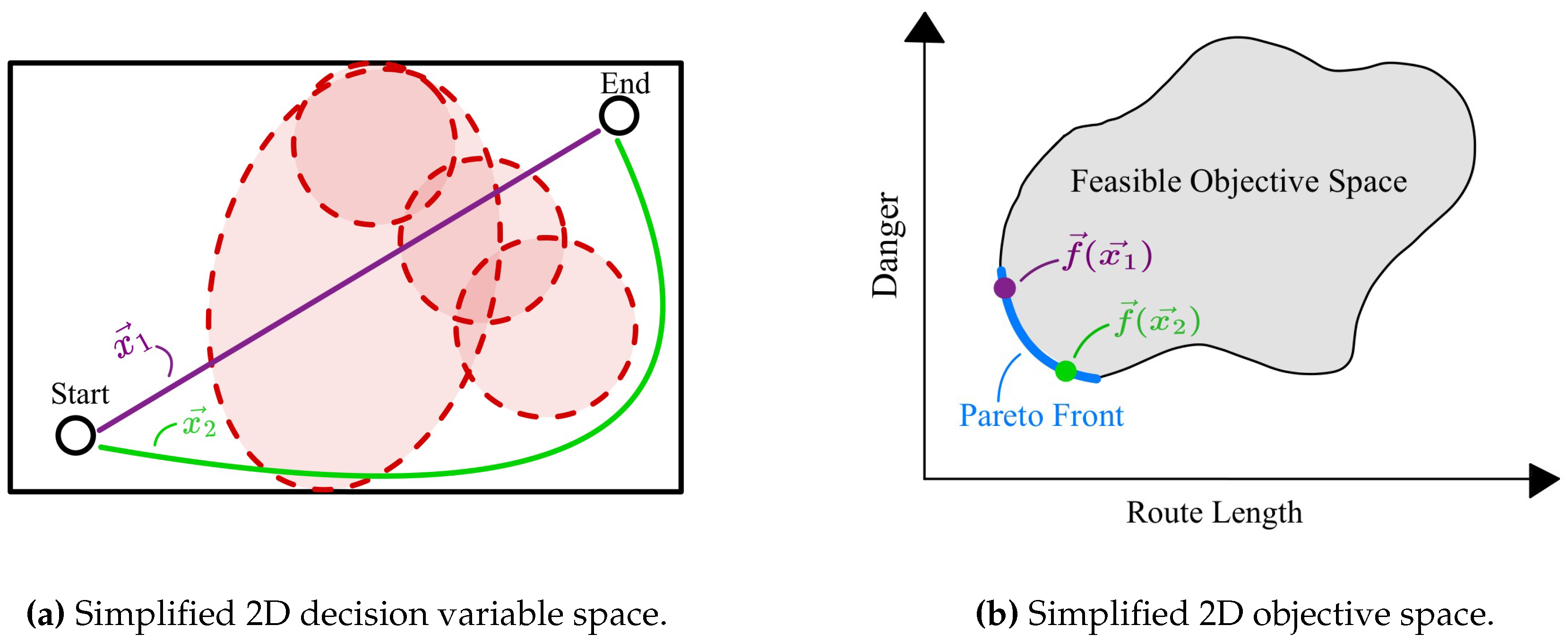
Figure 2.
Flow chart [16] of the paper selection process.
Figure 2.
Flow chart [16] of the paper selection process.
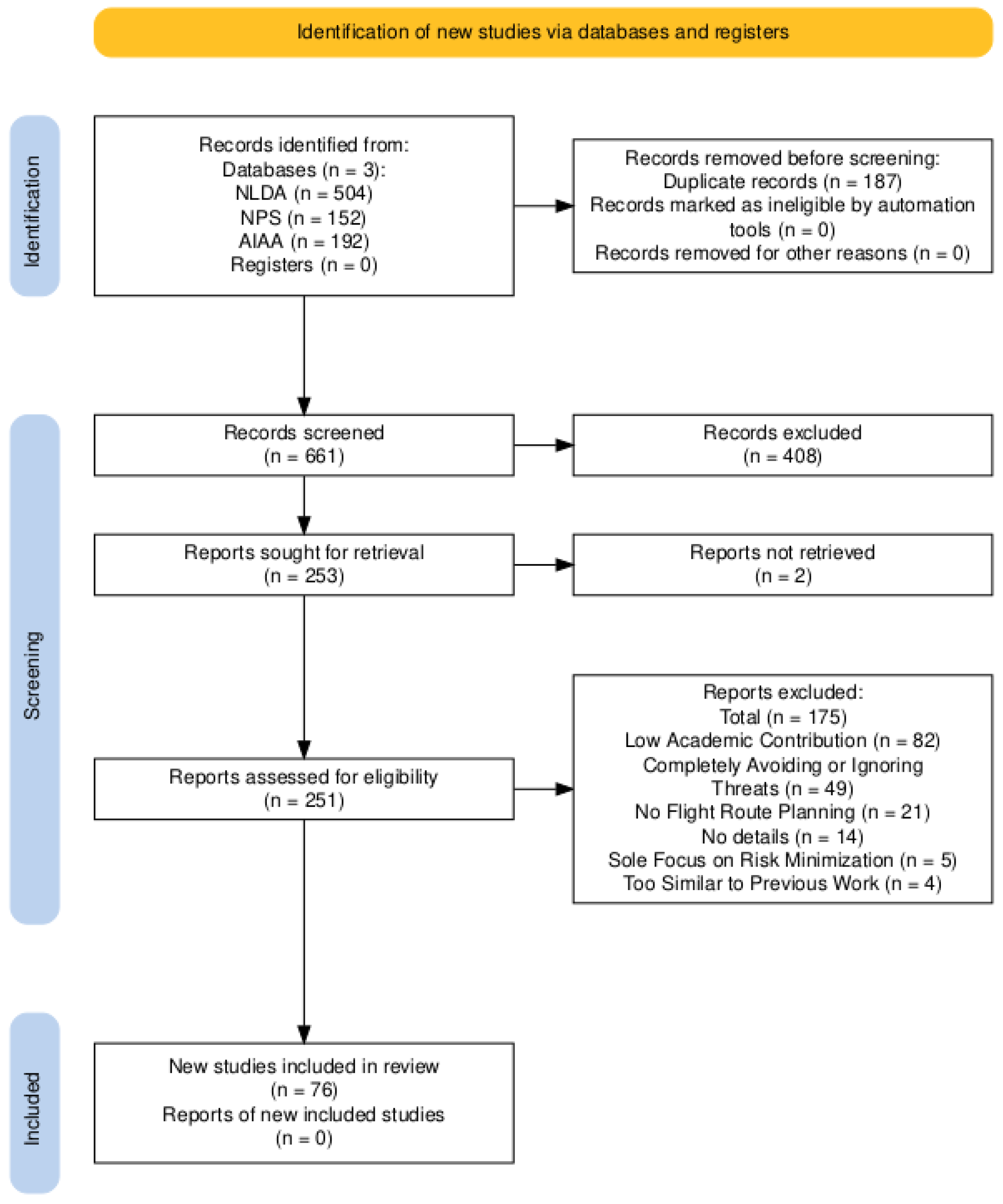
Figure 3.
Four different approaches of Preference Handling techniques.
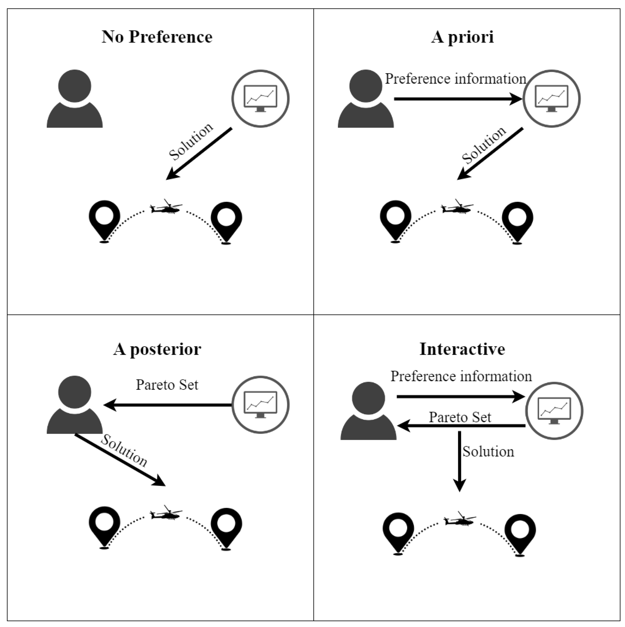
Figure 4.
Preference handling classes employed in the literature.
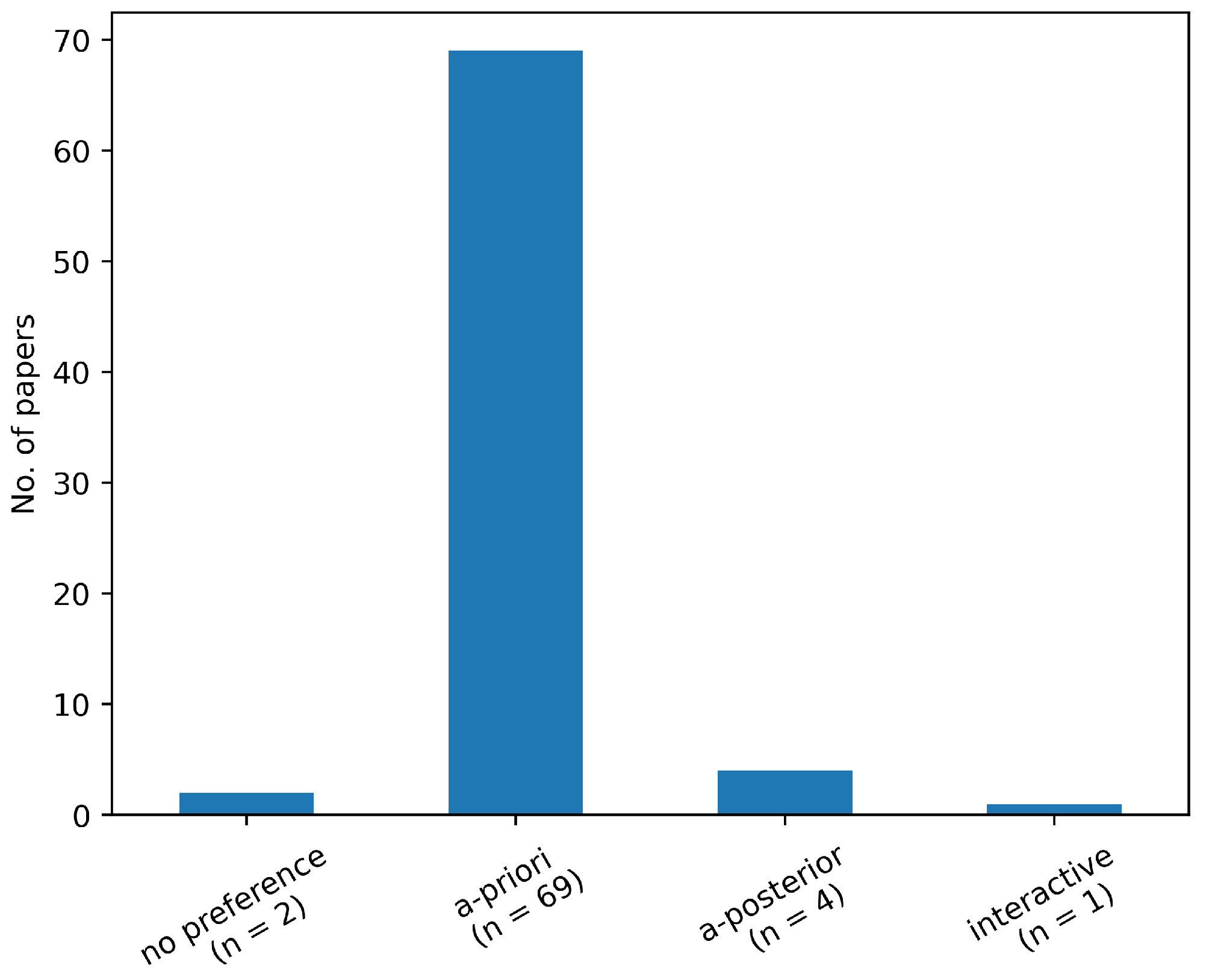
Figure 5.
Performance evaluation using preference information.
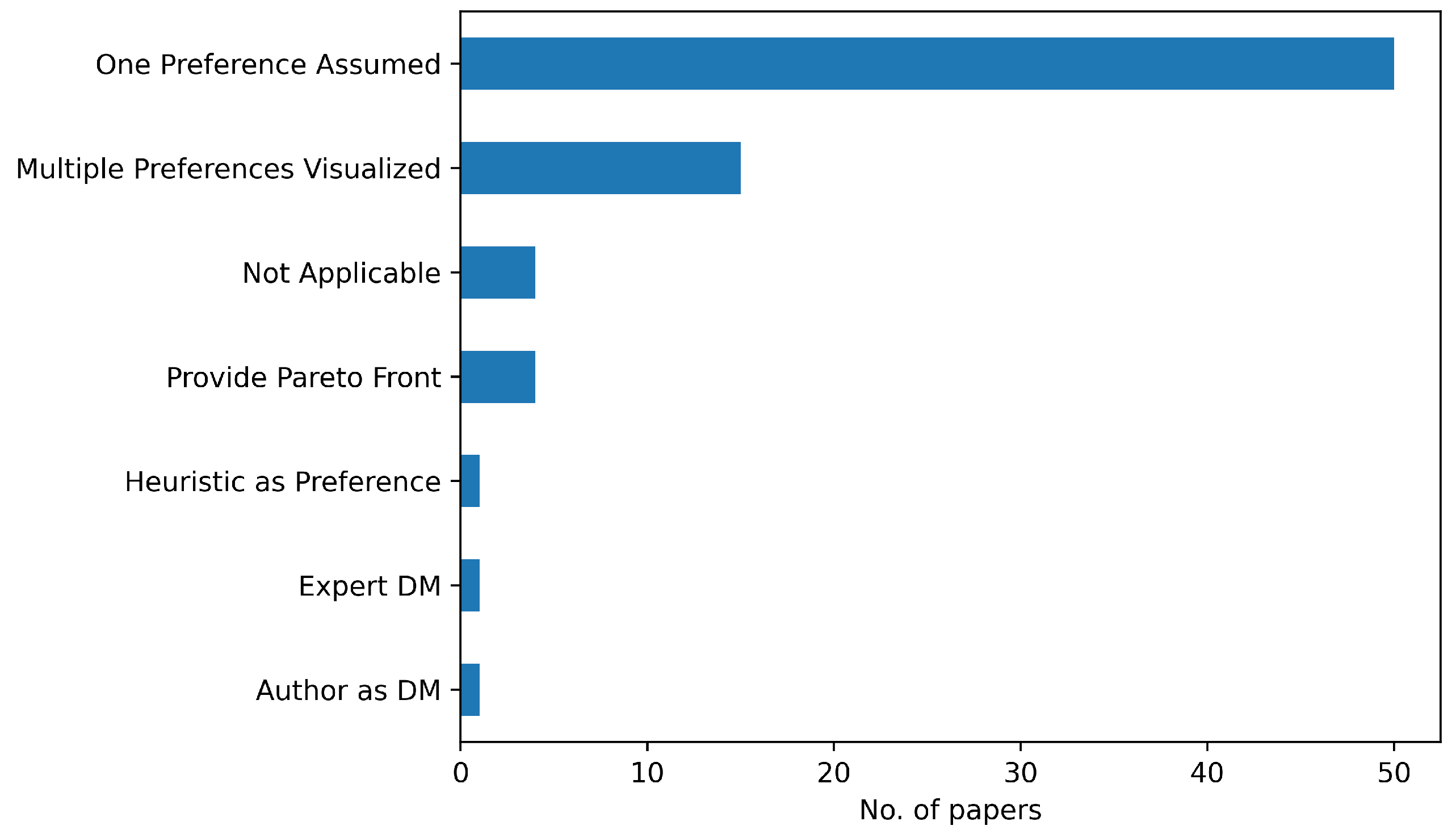
Figure 6.
Geometric interpretation of the Nash Product.
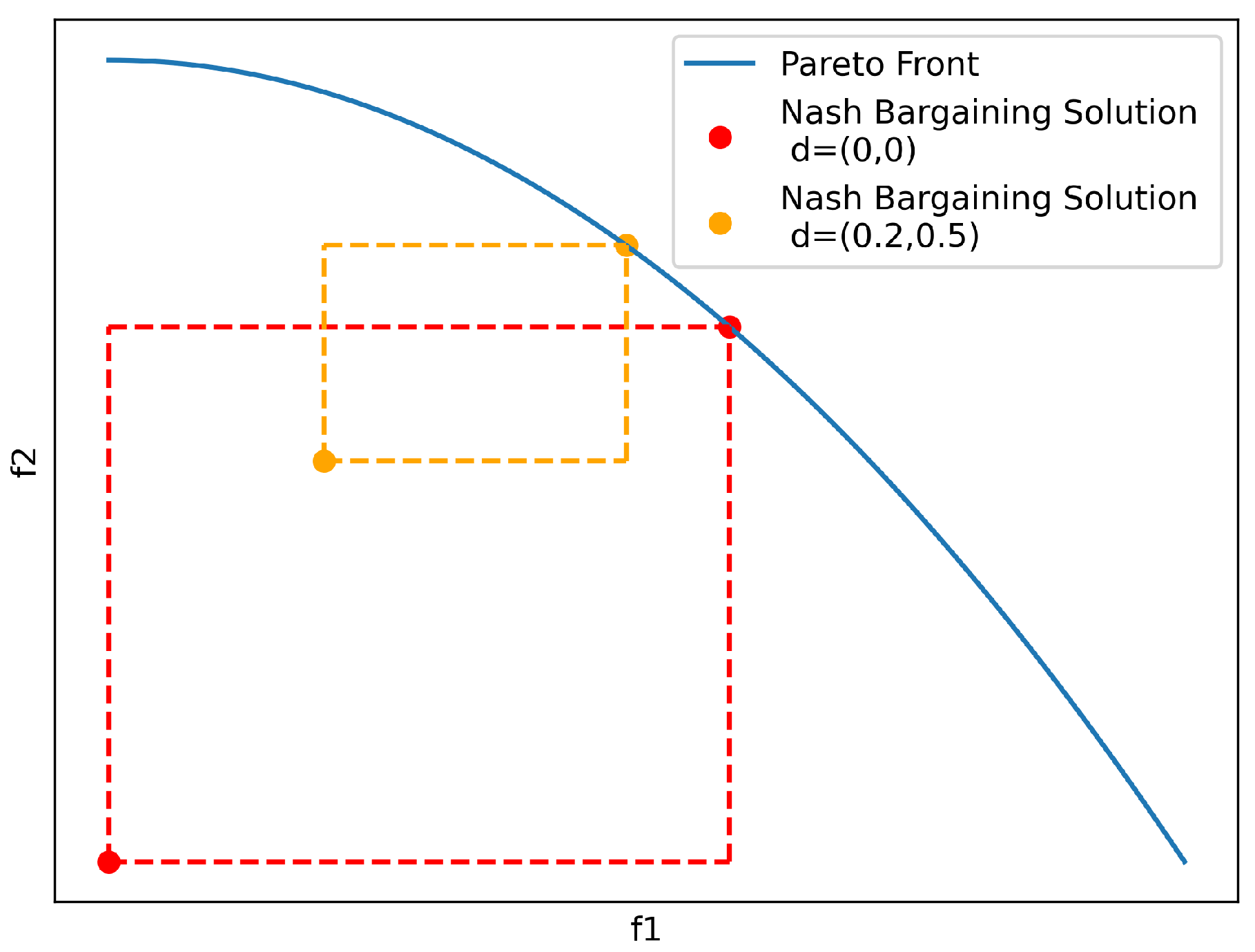
Figure 7.
Effect of changing the disagreement point.
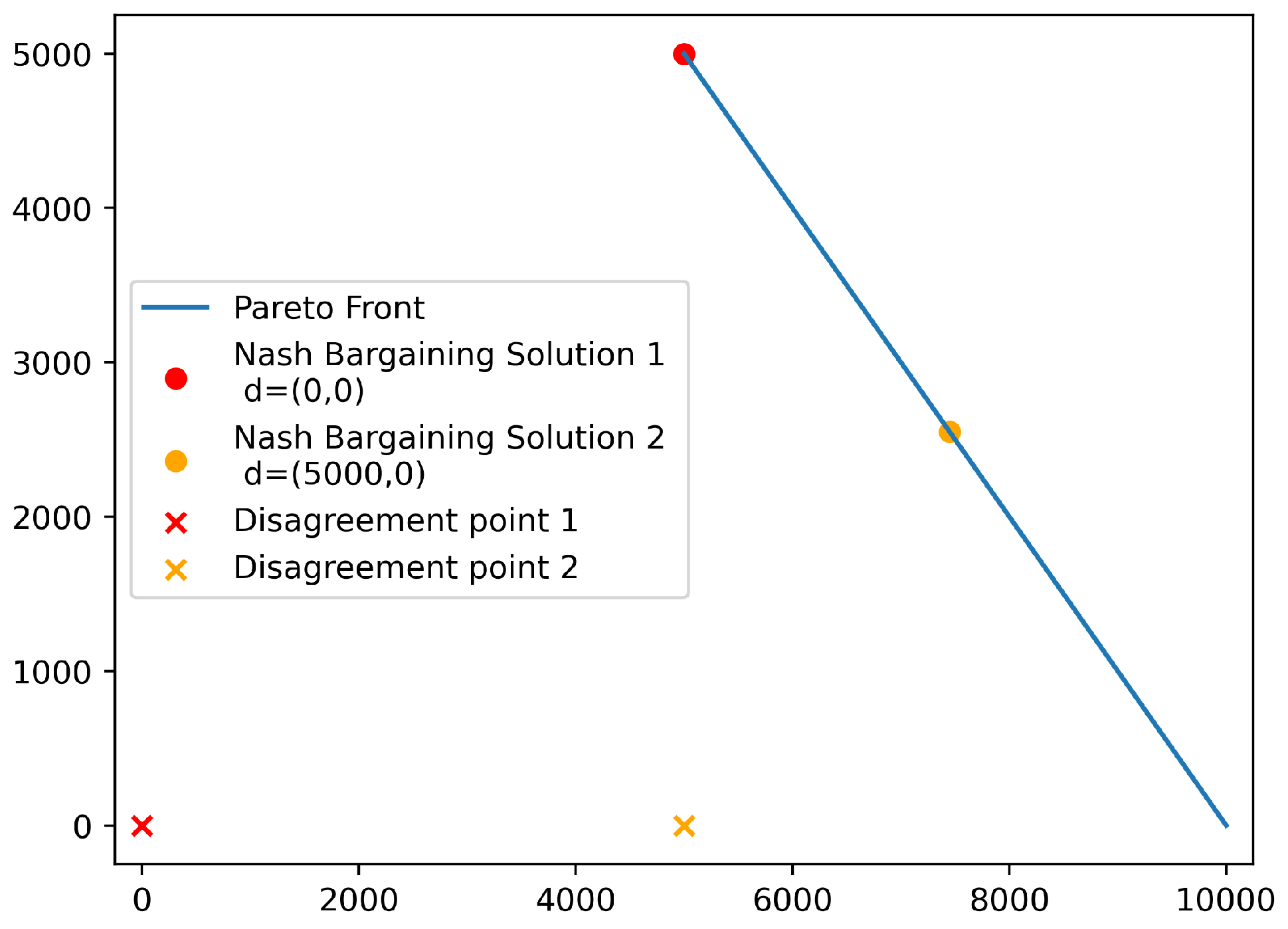
Figure 8.
a-priori preference handling methods in UAV path planning.
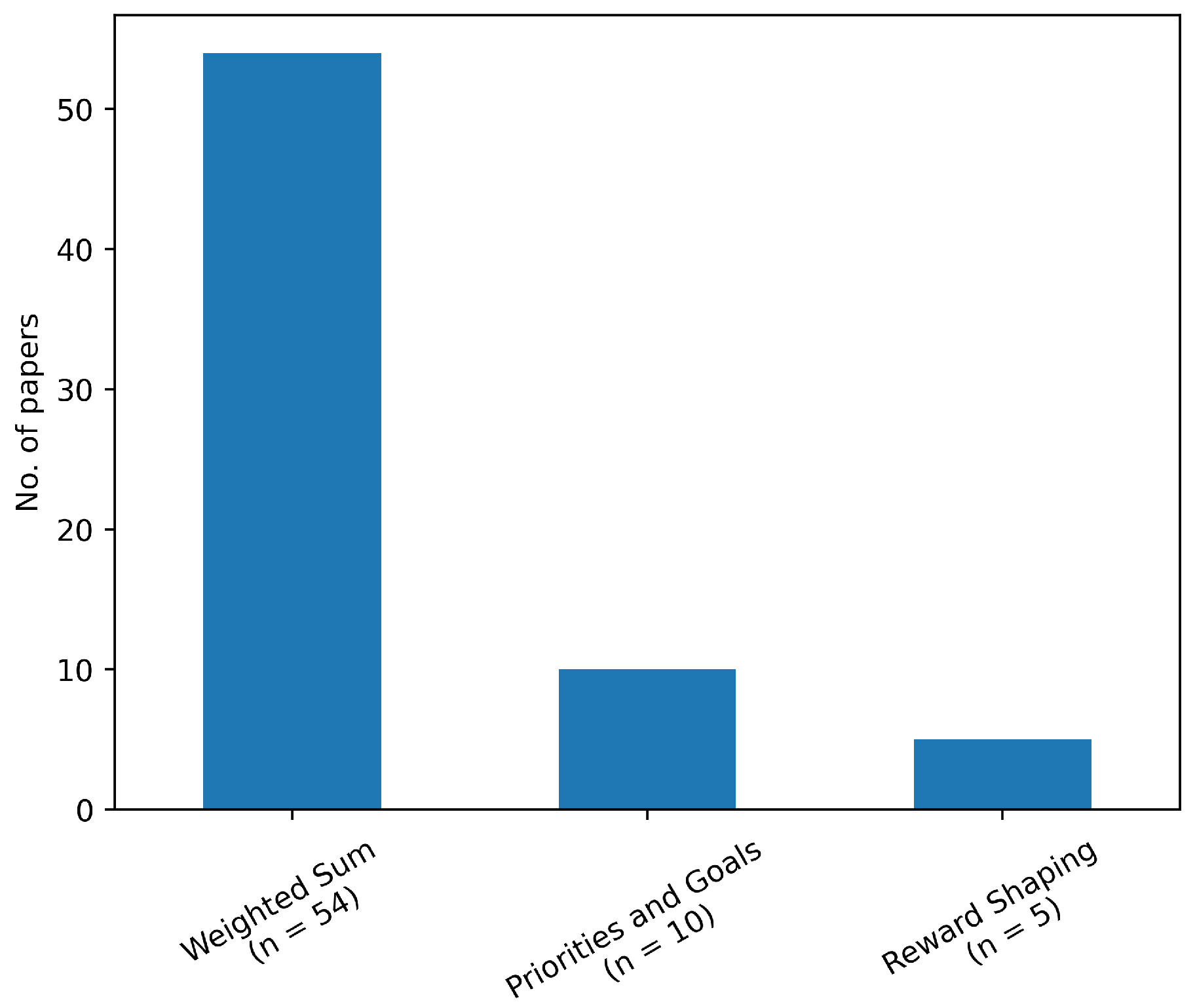
Figure 9.
Geometric interpretation of the Weighted Sum method on convex and non-convex feasible sets.
Figure 9.
Geometric interpretation of the Weighted Sum method on convex and non-convex feasible sets.
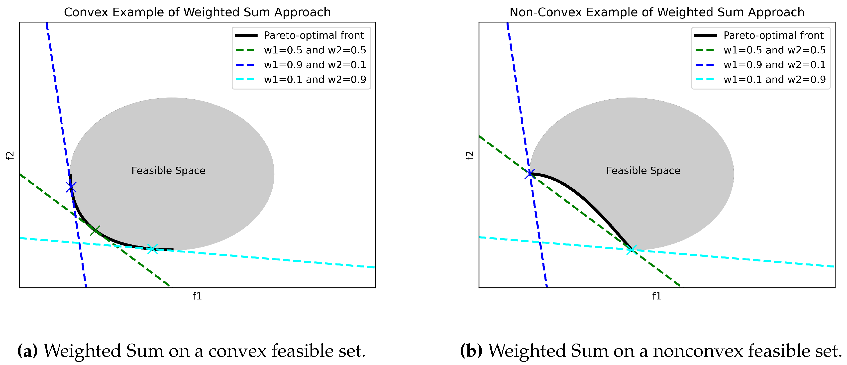
Figure 10.
Normalization of objective values before weight specification.
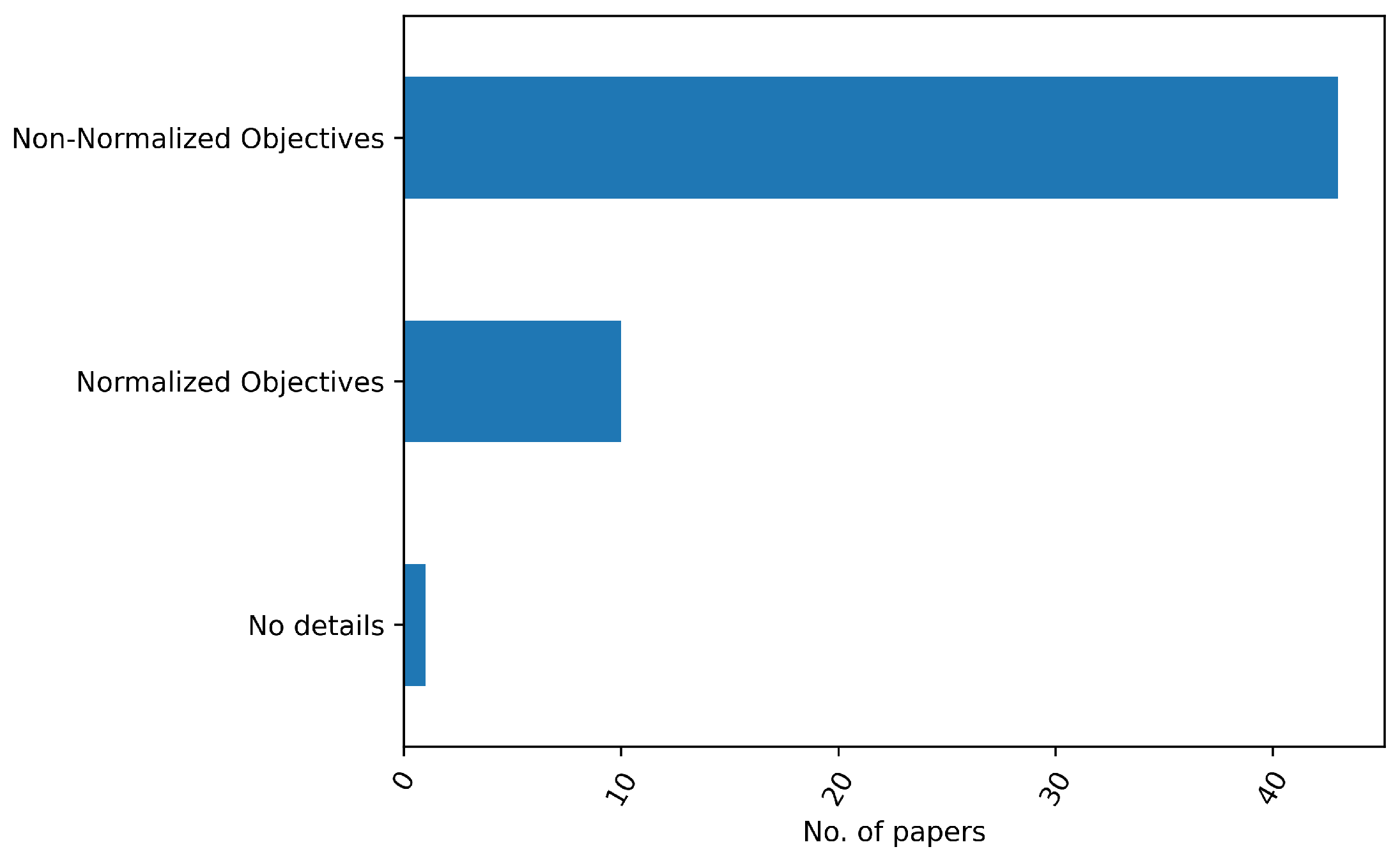
Figure 11.
Geometric interpretation of the -constraint method on a non-convex pareto front.
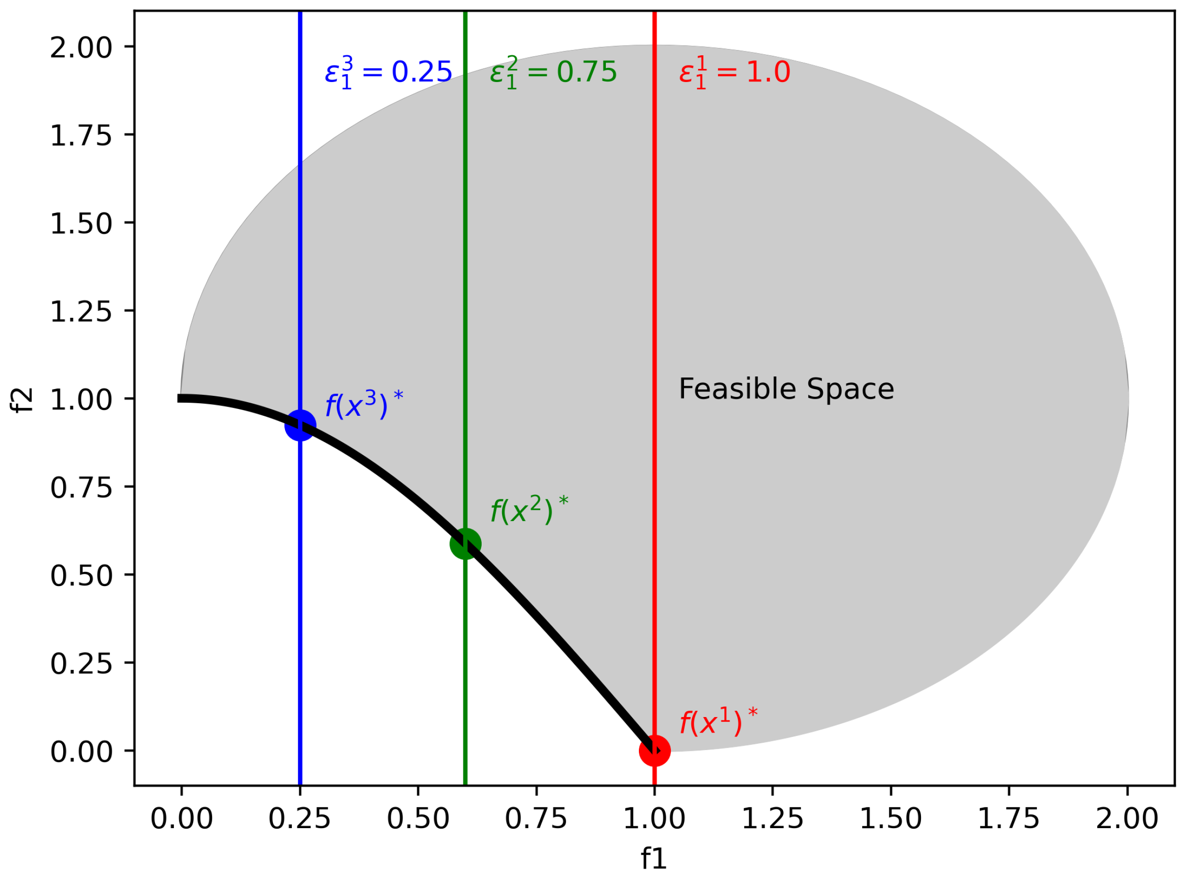
Table 1.
Focus of existing surveys.
| References | Year | OA | RR | OM | C | PH |
|---|---|---|---|---|---|---|
| Zhao et al. [14] | 2018 | ✓ | ✗ | ✗ | ✗ | ✗ |
| Song et al. [12] | 2019 | ✓ | ∼ | ∼ | ∼ | ∼ |
| Aggarwal & Kumar [9] | 2020 | ✓ | ✓ | ✗ | ✗ | ✗ |
| Saadi et al. [13] | 2022 | ✓ | ✗ | ∼ | ∼ | ✗ |
| Jones et al. [10] | 2023 | ✓ | ✓ | ✗ | ✗ | ✗ |
OA: Optimization Algorithm, RR: Route Representation, OM: Objective Modeling, C: Constraints, PH: Preference Handling; ✓: Concept covered, ∼: Concept introduced, ✗: Concept not covered.
Table 2.
Inclusion and exclusion criteria of the paper selection.
| Inclusion Criteria | Exclusion Criteria |
|---|---|
| Significant contribution to research ( Average yearly citations ≥ 1) |
Low academic impact (Average yearly citations < 1) |
| Threat as optimization objective | Completely avoid or ignore threats |
| Handle multiple objectives | Sole Focus on Threat or Distance minimization |
| Route planning in the flight domain | No route planning or different domain |
| Sufficient explanation of methodology | No details |
| Propose novel work | Minor change from existing work |
Disclaimer/Publisher’s Note: The statements, opinions and data contained in all publications are solely those of the individual author(s) and contributor(s) and not of MDPI and/or the editor(s). MDPI and/or the editor(s) disclaim responsibility for any injury to people or property resulting from any ideas, methods, instructions or products referred to in the content. |
© 2024 by the authors. Licensee MDPI, Basel, Switzerland. This article is an open access article distributed under the terms and conditions of the Creative Commons Attribution (CC BY) license (http://creativecommons.org/licenses/by/4.0/).
Copyright: This open access article is published under a Creative Commons CC BY 4.0 license, which permit the free download, distribution, and reuse, provided that the author and preprint are cited in any reuse.


