Research on the Algorithm of Tractor GNSS/INS Integrated Navigation System Assisted by CNN-BiLSTM

1. Introduction

As China’s agriculture transitions toward modernization, intelligence, and precision, the efficient utilization of existing land resources to increase food production has become one of the country’s most pressing agricultural challenges[1].Precision agriculture significantly enhances agricultural productivity, improves the quality of agricultural products, and reduces production costs, making it an effective means to boost food output[2,3].In the complex and ever-changing terrain of agricultural fields, coupled with diverse environmental conditions, traditional manual driving methods struggle to achieve precise task path control and efficient field management[4].As a result, in recent years, China has entered a period of rapid development in agricultural machinery autonomous navigation technology, with a focus on research in agricultural machine navigation and positioning. Studies have shown that the Global Navigation Satellite System (GNSS) can provide centimeter-level positioning accuracy in open environments[5].However, due to its limited signal penetration capability, GNSS is prone to signal loss when passing through densely wooded areas, resulting in a significant decline in positioning accuracy or even complete loss of positioning, thereby disrupting the normal operation of tractors. To address this issue, current mainstream agricultural machine navigation solutions typically combine GNSS with an Inertial Navigation System (INS), which offers autonomous navigation and robust resistance to interference[6].The GNSS/INS integrated navigation system leverages the strengths of both technologies to enhance positioning accuracy. INS relies on dead reckoning for navigation, offering advantages such as interference resistance, full autonomy, real-time performance, comprehensive output parameters, and high update frequency, all without the need for external information. However, the errors in INS accumulate over time, leading to a gradual decline in accuracy during long-duration navigation tasks.

GNSS and INS possess inherently complementary characteristics: GNSS provides all-weather, high-precision positioning, while INS offers comprehensive output information and high update rates. When GNSS signals are abundant, the integrated navigation system can use GNSS to correct the accumulated errors of INS, achieving high-precision navigation[7].However, under complex terrain or variable environmental conditions, GNSS signals may be extremely weak upon reaching the ground and are prone to interference, leading to signal failure. When GNSS signals cannot be properly received, the system switches to pure inertial navigation mode, relying solely on the INS for navigation information, without the ability to correct errors using external GNSS data. In such cases, the accumulated errors in the INS rapidly increase, causing the Kalman filter to struggle with properly fusing the observational data, ultimately resulting in a significant degradation of navigation accuracy[8].

In recent years, with the rapid development of Artificial Intelligence (AI) and Deep Learning technologies, Neural Networks (NN) have gained prominence due to their powerful ability to handle nonlinear problems and their capacity to approximate and fit functions to an infinite degree of accuracy[9]. Many researchers have integrated neural networks into integrated navigation systems to address the challenges posed by GNSS signal denial. To mitigate the significant degradation in positioning accuracy when GNSS signals are unavailable in GNSS/INS integrated navigation systems, some scholars have proposed methods that use genetic algorithm-optimized Radial Basis Function (RBF) neural networks to assist in navigation and positioning[10,11,12,13]. The input to the network consists of the position information output by the inertial navigation system (INS), while the output corresponds to the associated position error information. Some researchers have proposed fusion models using Back Propagation (BP) neural networks to assist integrated navigation systems[14,15,16]. Both of these algorithms attempt to improve navigation performance during GNSS outages by predicting INS errors using the current INS output. Their main drawback is that they struggle to learn long-term sequential features. When handling time-series data, they are unable to store more past dynamic information, resulting in a lack of prior dynamics in the time series data. Recurrent Neural Networks (RNN) can link past position information with the current output, making them effective for time-series data. Dai[17] and others used RNN to predict the position and velocity errors of INS, achieving an average improvement of 77% in navigation accuracy. However, during the training of RNNs, the repeated use of parameters can lead to issues such as gradient explosion and gradient vanishing. Long Short-Term Memory (LSTM) networks are an improved version of RNNs, incorporating memory cells and gating mechanisms to address the issues of gradient explosion and vanishing. LSTMs can capture long-term dependencies and have the ability to perform highly nonlinear dynamic mapping while effectively storing past information. Fang[18] and others proposed an algorithm based on Long Short-Term Memory (LSTM) neural networks to assist Strapdown Inertial Navigation Systems (SINS). However, this approach applies the same set of weight coefficients to fit and predict different positional outputs, such as longitude and latitude, from the INS. As a result, it does not achieve optimal performance.

To address the aforementioned issues, this paper first introduces the GNSS/INS integrated navigation system and the Extended Kalman Filter (EKF) technique used. Then, by thoroughly analyzing the characteristics of IMU dynamics measurement data and GNSS navigation data during tractor operations, a model combining Convolutional Neural Networks (CNN) and Bidirectional Long Short-Term Memory (BiLSTM) networks is designed to assist the integrated navigation system. By leveraging the characteristics of CNN convolution operations and weight sharing, this model extracts more local features from time-series data. Combined with Bidirectional LSTM, which models high-dimensional sequential features, the system enables accurate prediction of time-series data. This model can provide more stable integrated navigation positioning information even in the case of GNSS signal loss, thereby enhancing the reliability of the tractor GNSS/INS integrated navigation system in complex operational environments. Finally, the effectiveness of the algorithm is validated using real-field data from tractor simulations of agricultural operations. An experiment was designed with a 100-second GPS failure, using MAE and RMSE as evaluation metrics. The experimental results show that during the 100-second GPS outage, the proposed model effectively suppresses the accumulation of errors in integrated navigation positioning, and its fitting performance is comparable to that of GPS.

2. GNSS/INS Integrated Navigation System

2.1. Extended Kalman Filter

Kalman filtering, as a fundamental algorithm, is the top priority in the study of integrated navigation systems. Conventional Kalman filtering is based on linear mathematical models, requiring precise mathematical representations and accurate system and measurement noise characteristics. However, in agricultural field operations, such as tractor navigation through complex terrain and changing environments, obtaining accurate characteristics for measurement and system noise is challenging.

In such cases, where the navigation system is modeled by nonlinear dynamics, conventional Kalman filtering is not suitable. Instead, the EKF is employed to address the nonlinear nature of the system[19]. The EKF linearizes the nonlinear system by performing a first-order Taylor series expansion, followed by a linear truncation, yielding a linearized model of the system[20]. This linearized model is then used in the recursive equations of the conventional Kalman filter to estimate the system's state.

In summary, while the conventional Kalman filter works well for linear systems, the EKF provides an effective solution for nonlinear integrated navigation systems, such as those used in tractor operations, where the environment and dynamics are more complex and variable.

The state equation and measurement equation of the discretized nonlinear system model can be expressed as follows:

$$X_k=f\left(X_{k-1},k-1\right)+{\Gamma }_{k-1}{W}_{k-1}$$

(1)

$$Z_k=h\left(X_k,k\right)+V_k$$

(2)

Where $f\left(\cdot \right)$and $h\left(\cdot \right)$ are nonlinear functions, while $W_{k-1}$ and $V_k$ are the system noise vector and measurement noise vector, respectively. Both noise vectors are Gaussian white noise sequences with zero mean, and they are uncorrelated with each other. Expanding $f\left(X_{k-1}\right)$ and $h\left(X_k\right)$ as Taylor series around ${\stackrel{\wedge }{X}}_{k-1|k-1}$ and ${\stackrel{\wedge }{X}}_{k|k-1}$, respectively, and neglecting higher-order terms beyond the second, the following approximations are obtained:

$$f\left(X_{k-1}\right)=f\left({\stackrel{\wedge }{X}}_{k-1|k-1}\right)+{\displaystyle \frac{\partial f\left({\stackrel{\wedge }{X}}_{k-1|k-1}\right)}{\partial X}}\left(X_{k-1}-{\stackrel{\wedge }{X}}_{k-1|k-1}\right)$$

(3)

$$h\left(X_k\right)=h\left({\stackrel{\wedge }{X}}_{k|k-1}\right)+{\displaystyle \frac{\partial h\left({\stackrel{\wedge }{X}}_{k-1|k-1}\right)}{\partial X}}\left(X_{k-1}-{\stackrel{\wedge }{X}}_{k|k-1}\right)$$

(4)

Let:

$${\varphi }_{k|k-1}={\displaystyle \frac{\partial f\left({\stackrel{\wedge }{X}}_{k-1|k-1}\right)}{\partial X}}$$

(5)

$$H_k={\displaystyle \frac{\partial h\left({\stackrel{\wedge }{X}}_{k-1|k-1}\right)}{\partial X}}$$

(6)

After constructing the state equation and measurement equation, and obtaining the linearized state transition matrix and observation matrix, the Kalman filter proceeds with two main steps: Time Update and Measurement Update.

The time update is used to predict the state estimate and its covariance at the next time step based on the current state and control input. The equations for the time update are as follows:

The state prediction at time step $k$ based on the state estimate at time step $k-1$ can be expressed as follows:

$${\stackrel{\wedge }{X}}_{k|k-1}=f\left({\stackrel{\wedge }{X}}_{k-1|k-1}\right)$$

(7)

To compute the covariance matrix at time step $k$, the following equation is used:

$$P_{k|k-1}={\varphi }_{k,k-1}{P}_{k-1}{\varphi }_{k,k-1}^T+{\Gamma }_{k-1}{Q}_{k-1}{\Gamma }_{k-1}^T$$

(8)

The measurement update step is used to correct the predicted state and covariance based on the new measurement obtained from the system. The equations for the measurement update are as follows:

To compute the Kalman Gain at time step $k$, the following equation is used:

$$K_k=P_{k|k-1}{H}_k^T{\left(H_k{P}_{k|k-1}{H}_k^T+R_k\right)}^{-1}$$

(9)

From the state prediction value at time $k$,${\stackrel{\wedge }{X}}_{k|k-1}$, obtain the state estimation value at time $k$, ${\stackrel{\wedge }{X}}_k$:

$${\stackrel{\wedge }{X}}_k={\stackrel{\wedge }{X}}_{k|k-1}+K_k\left(Z_k-h\left({\stackrel{\wedge }{X}}_{k|k-1}\right)\right)$$

(10)

To update the system's covariance matrix at time step $k$, the following equation is used:

$$P_k=\left(I-K_k{H}_k\right)P_{k|k-1}{\left(I-K_k{H}_k\right)}^T+K_k{R}_k{K}_k^T$$

(11)

Or:

$$P_k=\left(I-K_k{H}_k\right)P_{k|k-1}$$

(12)

From the above formulas, it can be observed that given the initial state variable ${\stackrel{\wedge }{X}}_0$ and its corresponding variance $P_0$, the state variable ${\stackrel{\wedge }{X}}_k$ for the next moment can be derived based on the observation $Z_k$ at the current moment.

In the Kalman filter equations, the main calculations involve the gain equation and the state estimation equation. The gain calculation only requires the variance from the previous moment, but the state estimation prediction requires the gain $K_k$ obtained in the previous step. By examining the Kalman filter formulas, each estimate is derived based on the results from the preceding moment, thereby forming an iterative estimation process in a closed-loop structure.

The estimated error is fed back into the INS to correct its output. This structure, which maintains the error within a small range and satisfies the linearity assumptions of the Kalman filter, is the optimal choice for such systems.

2.2. Mathematical Model for GNSS/INS Loose Coupling Navigation

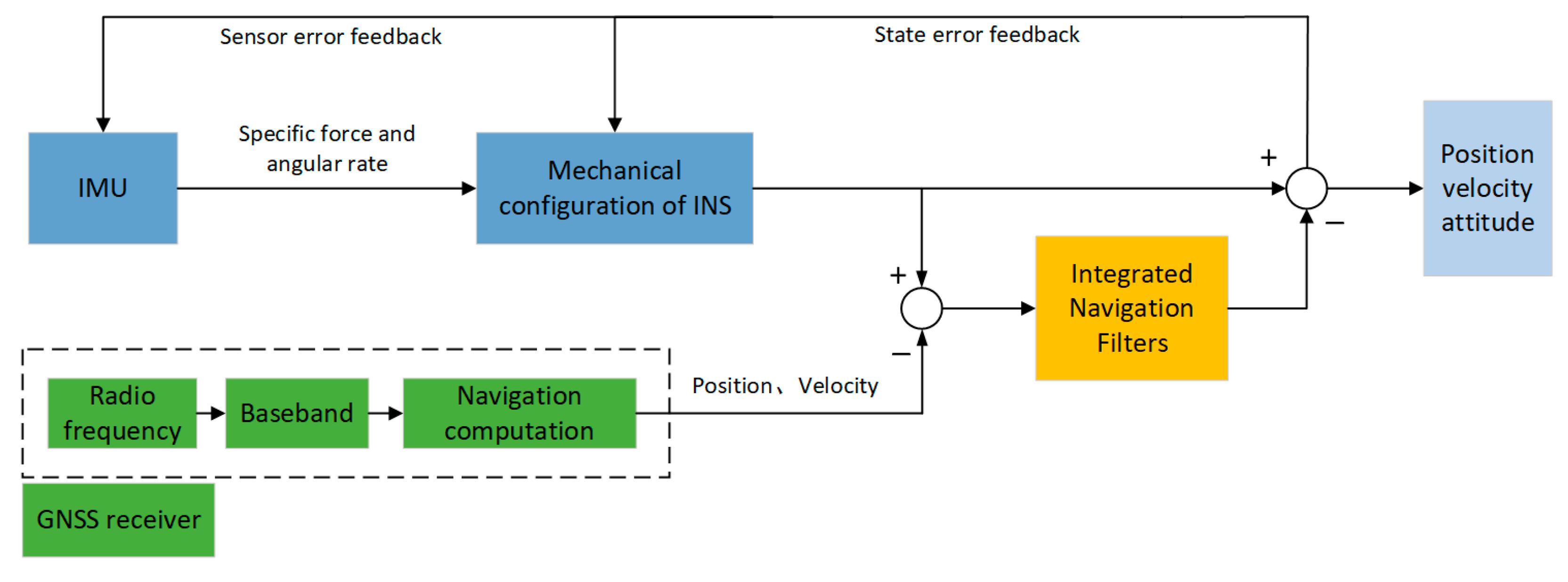
The tractor's combined navigation system studied in this paper adopts a loose coupling approach. The GNSS/INS loose coupling process is shown in Figure 1. The IMU outputs acceleration and angular velocity, which are processed by the INS to output velocity, position, and attitude information. Meanwhile, GNSS provides position information through navigation solutions and velocity information through Doppler speed measurements. If the sensor outputs (such as the position information calculated by the IMU and GPS position information) are directly used as inputs to the Kalman filter, it would increase the complexity of the state and measurement equations.

The error values obtained by subtracting the two sources simplify the filter design. In this approach, the Kalman filter only needs to estimate the change in errors rather than computing the complete state. The residuals after the subtraction are fused by the Kalman filter to estimate the INS errors, which are then used to correct the results from the INS. The corrected navigation information is output as the final result, while the estimated IMU bias error is fed back to the IMU to correct the IMU errors[21].

（1）State Model of the Integrated Navigation System：

In loosely coupled GNSS/INS integration, error-state Kalman filtering is used for navigation solution computation. Therefore, the Kalman filter's state vector includes navigation state errors and sensor errors, defined as：

$$\delta x\left(t\right)={\left[{\left(\delta r^n\right)}^T {\left(\delta v^n\right)}^T {\varphi }^T b_g^T b_a^T s_g^T s_a^T\right]}^T$$

(13)

Where $\delta r^n$ is position error vector of the inertial navigation system (INS). $\delta v^n$is velocity error vector of the INS. $\varphi$ is attitude error vector of the INS. $b_g$ is bias vector of the three-axis gyroscope. $b_a$ is bias vector of the three-axis accelerometer. $s_g$ is scale factor error vector of the gyroscope. $s_a$ is scale factor error vector of the accelerometer.

Based on the SINS error model and the linearization process described earlier, the state-space equation for the loosely coupled Kalman filter can be expressed as follows:

$$\delta \stackrel{•}{x}(t)=F(t)\delta x(t)+G(t)w(t)$$

(14)

Where $F(t)$ represents the system state transition matrix, which characterizes the dynamic relationship between the state variables over time. $G(t)$ is the system noise projection matrix, mapping the impact of system noise into the state space. $w(t)$ denotes the system noise vector, assumed to follow a zero-mean Gaussian distribution.

The discretized system state equation can be written as:

$$\delta x_k={\varphi }_{k|k-1}\delta x_{k-1}+{\Gamma }_{k-1}{\omega }_{k-1}$$

(15)

Where $x_k$and$x_{k-1}$ represent the state vectors at time steps $k$ and $k-1$, respectively.${\varphi }_{k|k-1}$ is the discretized state transition matrix, ${\Gamma }_{k-1}$ is the system noise driving matrix, ${\omega }_{k-1}$ is the system noise vector.

（2）Integrated navigation system observation model:

The relationship between the GNSS antenna phase center and the IMU measurement center, in terms of position transformation, takes into account the lever arm effect (the offset between the phase center of the GNSS antenna and the IMU measurement center). This correction is necessary because GNSS provides the position of the antenna phase center, while the IMU provides the position based on the IMU measurement center.

The position transformation equation that accounts for the lever arm effect is typically expressed as:

$$r_G^n=r_I^n+D_R^{-1}{C}_b^n{l}^b$$

(16)

$$D_R^{-1}=diag({[{\displaystyle \frac{1}{R_M+h}}\hspace{0.33em}\hspace{0.33em}{\displaystyle \frac{1}{(R_N+h)\cos \phi }}\hspace{0.33em}\hspace{0.33em}-1]}^T)$$

(17)

Where $r_G$ is the position vector of the GNSS antenna phase center. $r_I$ is the position vector of the IMU measurement center. $l^b$ represents the lever arm vector of the GNSS antenna, specifically the vector pointing from the IMU measurement center to the GNSS antenna phase center, expressed in the body frame (b-frame). This vector can be precisely measured and calibrated using high-precision measurement techniques.

The GNSS position observation equation can be expressed as follows:

$$\delta z_r=H_r\delta x+n_r$$

(18)

Where $H_r$ is the observation matrix that maps the system state vector $\delta x$ to the GNSS measurement space. $H_r=[I_3\hspace{0.33em}\hspace{0.33em}{0}_3\hspace{0.33em}\hspace{0.33em}(C_b^n{l}^b{\rm X})\hspace{0.33em}\hspace{0.33em}{0}_3\hspace{0.33em}\hspace{0.33em}{0}_3\hspace{0.33em}\hspace{0.33em}{0}_3\hspace{0.33em}\hspace{0.33em}{0}_3]$. $n_r$ is the measurement noise vector, assumed to follow a Gaussian distribution with zero mean and known covariance.

3. Neural Network-Assisted GNSS/INS Algorithm

3.1. BiLSTM Network Architecture

During tractor operations, the navigational data from sensors is collected at a specific sampling rate, forming a series of time-sequenced data. This data exhibits distinct spatiotemporal correlations, as the generation and variation of errors are intrinsically linked to past states. The Recurrent Neural Network (RNN) is a time-cyclic neural network endowed with memory and feedback capabilities. Its architecture enables the connection of present information with past data, allowing predictions of the current state based on both the current input and recent information. RNNs are widely applied in time-series forecasting. However, the repeated use of weight coefficients during training often leads to issues such as gradient explosion or vanishing gradients, thereby compromising the training efficacy. To address this issue, researchers have proposed several improved RNN models, among which the Long Short-Term Memory Network (LSTM) introduces a gating mechanism. These gates, functioning as control units, effectively mitigate gradient explosion and vanishing problems by selectively remembering and forgetting information. LSTMs possess the ability to perform highly nonlinear dynamic mapping and retain past information, making them particularly well-suited for handling extensive and long-term time-series data[22,23].

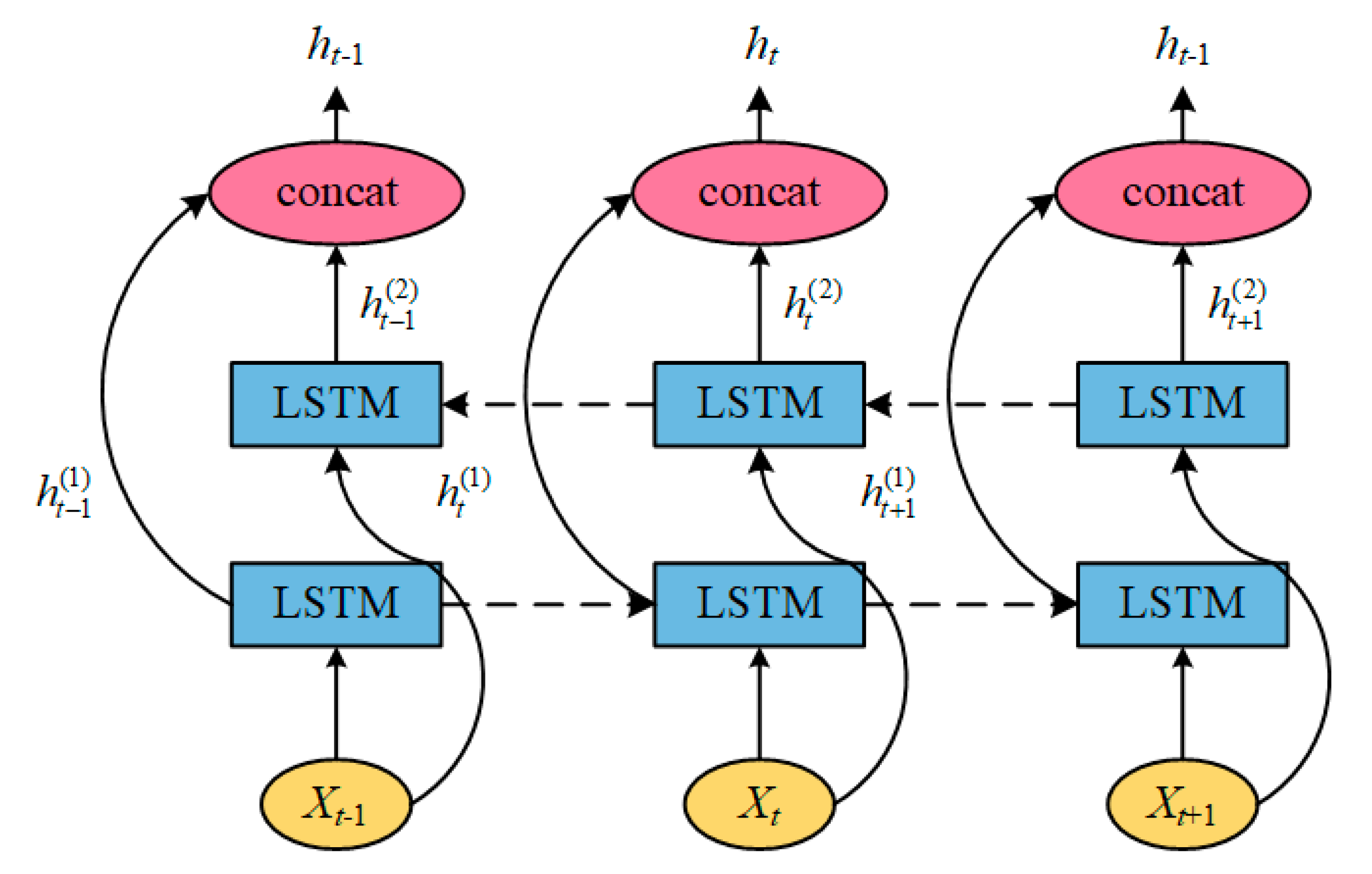
In the autonomous tractor navigation system, environmental factors such as slope variations or resistance differences during turns tend to have a cumulative effect on positioning errors. These effects are often linked to past states and the characteristics of the regions the tractor is about to enter. To address this, a combination of forward LSTM and backward LSTM networks, collectively known as the Bidirectional Long Short-Term Memory Network (BiLSTM), is introduced. The structure of BiLSTM is illustrated in Figure 2. The Bidirectional LSTM (BiLSTM) can extract positional data features from both past and future contexts, a capability that is particularly crucial during tractor operations. Its principle lies in combining the outputs of two LSTM layers: one processes the forward flow of the time-series data (from past to future), while the other handles the reverse flow (from future to past). At each time step, the outputs of the forward and backward LSTM units are concatenated to form a new state vector. This concatenated vector, enriched with bidirectional dependencies, provides a more comprehensive representation of the sequence data. This design significantly enhances the model's ability to capture intricate temporal relationships, making it well-suited for managing the dependencies inherent in long-term sequential data. When the tractor enters an area of obstruction or signal interference, the Bidirectional LSTM (BiLSTM) can leverage subsequent interference-free data to correct preceding errors, whereas a unidirectional LSTM can only infer based on past data[24,25]. Consequently, in scenarios where positioning data is subject to interference or fluctuations, the BiLSTM is more effective at mitigating the impact of error accumulation on subsequent positioning.

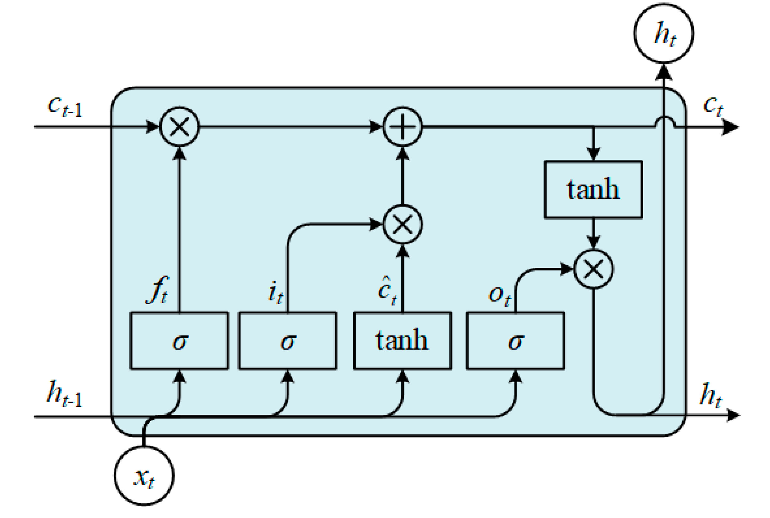
The fundamental units of the BiLSTM structure remain LSTM memory cells. Figure 3 illustrates the basic structure of an LSTM network.

The computational process of the LSTM structure is as follows:

$$f_t=\sigma (W_{xf}{x}_t+W_{hf}{h}_{t-1}+b_f)$$

(19)

$$i_t=\sigma (W_{xi}{x}_t+W_{hi}{h}_{t-1}+b_i)$$

(20)

$$\stackrel{\wedge }{c_t}=\tanh (W_{xc}{x}_t+W_{hc}{h}_{t-1}+b_c)$$

(21)

$$o_t=\sigma (W_{xo}{x}_t+W_{ho}{h}_{t-1}+b_o)$$

(22)

$$c_t=f_t\odot c_{t-1}+{\stackrel{\wedge }{c}}_t\odot i_t$$

(23)

$$h_t=o_t\odot m_t$$

(24)

Where $x_t$ represents the element value of the input sequence at time $t$, which is the input vector. $c$ refers to the memory cell, the core of the network.$f_t$ is the forget gate, which determines how much of the old memory to retain. $i_t$ is the update gate, deciding which short-term memories to forget and how much new memory to retain. $o_t$ is the output gate, which controls how much of $c_t$, the current state, is passed to the output. $h_{t-1}$ denotes the hidden state at time $t-1$. $\sigma$ represents the sigmoid activation function, and $\tanh$ denotes the hyperbolic tangent activation function, which helps prevent gradient explosion or vanishing. $W_{xi}$、$W_{xf}$、$W_{xo}$、$W_{xc}$ represent the weight vectors from the input layer to the input gate, forget gate, output gate, and memory cell, respectively. $W_{hi}$、$W_{hf}$、$W_{ho}$、$W_{hc}$ denote the weight vectors from the hidden layer to the input gate, forget gate, output gate, and memory cell, respectively.

3.2. CNN Network Architecture

In the context of a tractor's actual operations, the agricultural environment is both complex and ever-changing. Factors such as terrain undulations, soil moisture variations, and fluctuations in speed can give rise to intricate, nonlinear positioning errors. A standalone bidirectional LSTM captures the global temporal changes in the input data, yet it falls short in adequately extracting the local features of the data. Therefore, we integrate Convolutional Neural Networks (CNN) with BiLSTM. The CNN, with its sliding convolutional kernels along the temporal dimension, is adept at recognizing patterns within short time intervals in the navigation data, such as subtle variations in acceleration or angular velocity. Moreover, during tractor operations, positioning data is often subject to various sources of noise, particularly in areas with unstable signals or obstructions. CNNs excel in noise reduction by extracting key features and eliminating redundant information, thereby enabling the BiLSTM to more accurately process the time series data related to the tractor's operational status. This CNN-BiLSTM combination not only allows the model to focus on short-term local features but also facilitates the modeling of global temporal patterns. Furthermore, it enhances the model's robustness against interference in dynamic agricultural environments, leading to superior positioning accuracy in tractor navigation tasks[26].

The convolutional neural network consists of convolutional layers, pooling layers, fusion layers, and fully connected layers. Within this architecture, the convolutional layers contain kernels of varying sizes, which slide across the input data and perform convolution operations to extract fundamental local IMU features. The pooling layer serves to reduce the spatial dimensions of the feature maps, enhancing the network's noise resistance and reducing the number of parameters. Common pooling operations include max pooling and average pooling. In this case, max pooling is employed to reduce the dimensionality of the high-dimensional IMU dynamic data, extracting the maximum feature values. These are then fused in the fusion layer, followed by the integration of the learned high-level features in the fully connected layer, which produces the final prediction. In theory, the data is ultimately output through the fully connected layer; however, in this study, it is used solely to extract local spatial data features and to perform dimensionality reduction and noise reduction[27]. Consequently, the data post-pooling is fed into a BiLSTM network for temporal processing, and the fully connected layer outputs the results after BiLSTM processing.

The convolution operation can be expressed as:

$$Y\left(i\right)={\displaystyle \sum _{j=0}^{K-1}X}\left(i+j\right)\cdot W\left(j\right)$$

(25)

Here, the input sequence $X=\left[w^b a^b V^b P^b\right]$，K is the size of the convolutional kernel, which defines the length of the filter. $X\left(i+j\right)$ denotes the value of the input sequence at position $i+j$. $W\left(j\right)$ represents the parameter of the convolutional kernel at position $j$. $Y\left(i\right)$ is the output of the convolution operation at position $i$.

After convolution, an activation function such as ReLU (Rectified Linear Unit) is applied to introduce non-linearity into the model:

$$f(x)=\max (0,x)$$

(26)

For max pooling:

$$Y\left(i\right)=\underset{0\le j<p}{\max }\left(i\cdot s+j\right)$$

(27)

Where $p$ represents the size of the pooling window, and $s$ denotes the stride of the pooling operation.

3.3. CNN-BiLSTM Temporal Prediction Neural Network Architecture

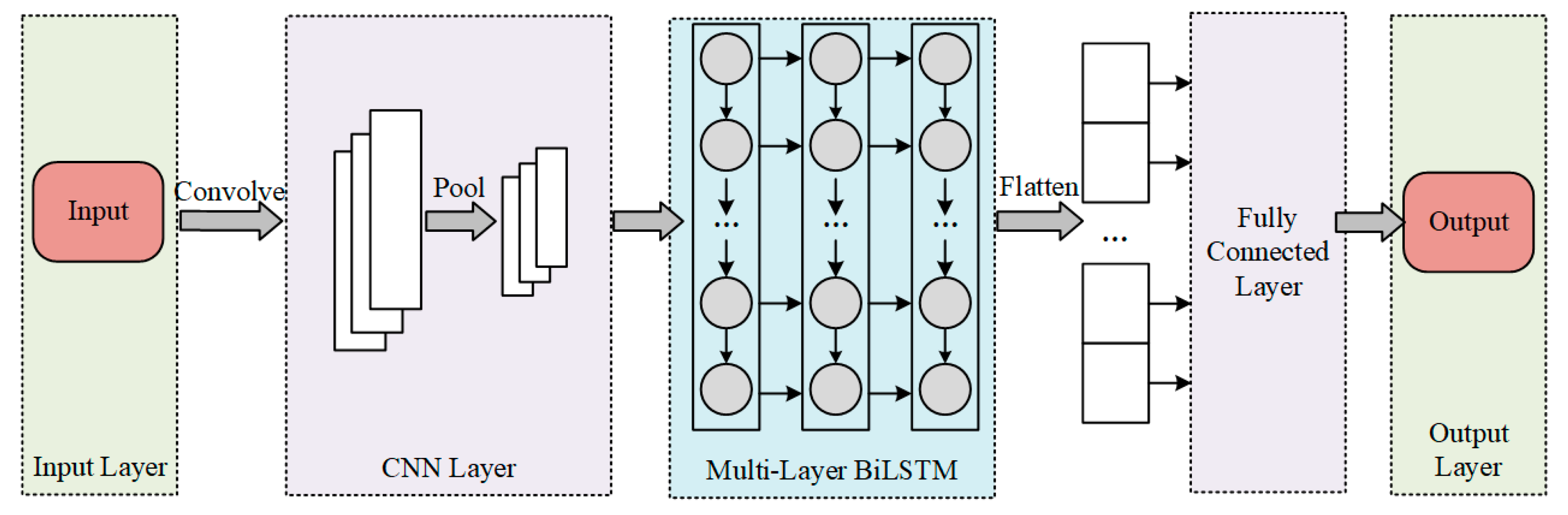
The CNN-BiLSTM architecture proposed in this paper is illustrated in Figure 4. The overall structure of the CNN-BiLSTM network encompasses several key components: the input (IMU dynamical measurement data, including acceleration and angular velocity information), data preprocessing (data integration and cleaning), convolutional neural network (comprising convolutional layers and pooling layers), bidirectional long short-term memory network (including BiLSTM layers, dropout layers, and fully connected layers), and the output (position increments and velocity predictions).

This structure begins by inputting the raw IMU data, followed by data preprocessing to eliminate outliers and remove redundant values. The processed data then undergoes spatial feature extraction via the CNN, after which it is fed into the Bidirectional Long Short-Term Memory (BiLSTM) layer. This layer processes the time series both forwards and backwards, effectively capturing the temporal dynamics and long-range dependencies within the data. By considering both past and future information, it ensures that the model comprehensively understands the data’s evolution, offering both depth and breadth for time series analysis[28]. Finally, the fully connected layer outputs the predicted values.

The hyperparameters of the CNN-BiLSTM model are as follows: The size of the convolutional layer is set to 3, indicating the use of a sliding window of size 3 along the time series dimension, with a stride of 1, meaning that local features are extracted with each step of 1 in the time dimension. The number of convolutional filters is set to 64. The pooling kernel size is set to 2, with a pooling stride of 2, meaning that the sequence length is compressed by sliding 2 time steps at a time. MaxEpochs represents the maximum number of iterations, with one epoch referring to a complete pass over the entire training dataset. The larger this value, the longer the training time, and it is set to 100. MiniBatchSize is a critical parameter that controls both the training speed and stability. It defines the number of samples used for each model update, thus regulating the frequency of model parameter updates and the scale of data sample processing during each training iteration; it is set to 8. InitialLearnRate is an important factor for ensuring fast and stable convergence of the model. By experimentally adjusting the learning rate and combining it with a learning rate decay strategy, the model can converge rapidly in the early stages of training and steadily approach the optimal solution in the later stages; it is set to 0.001. GradientThreshold controls the magnitude of the gradient to prevent gradient explosion during backpropagation, and it is set to 1.

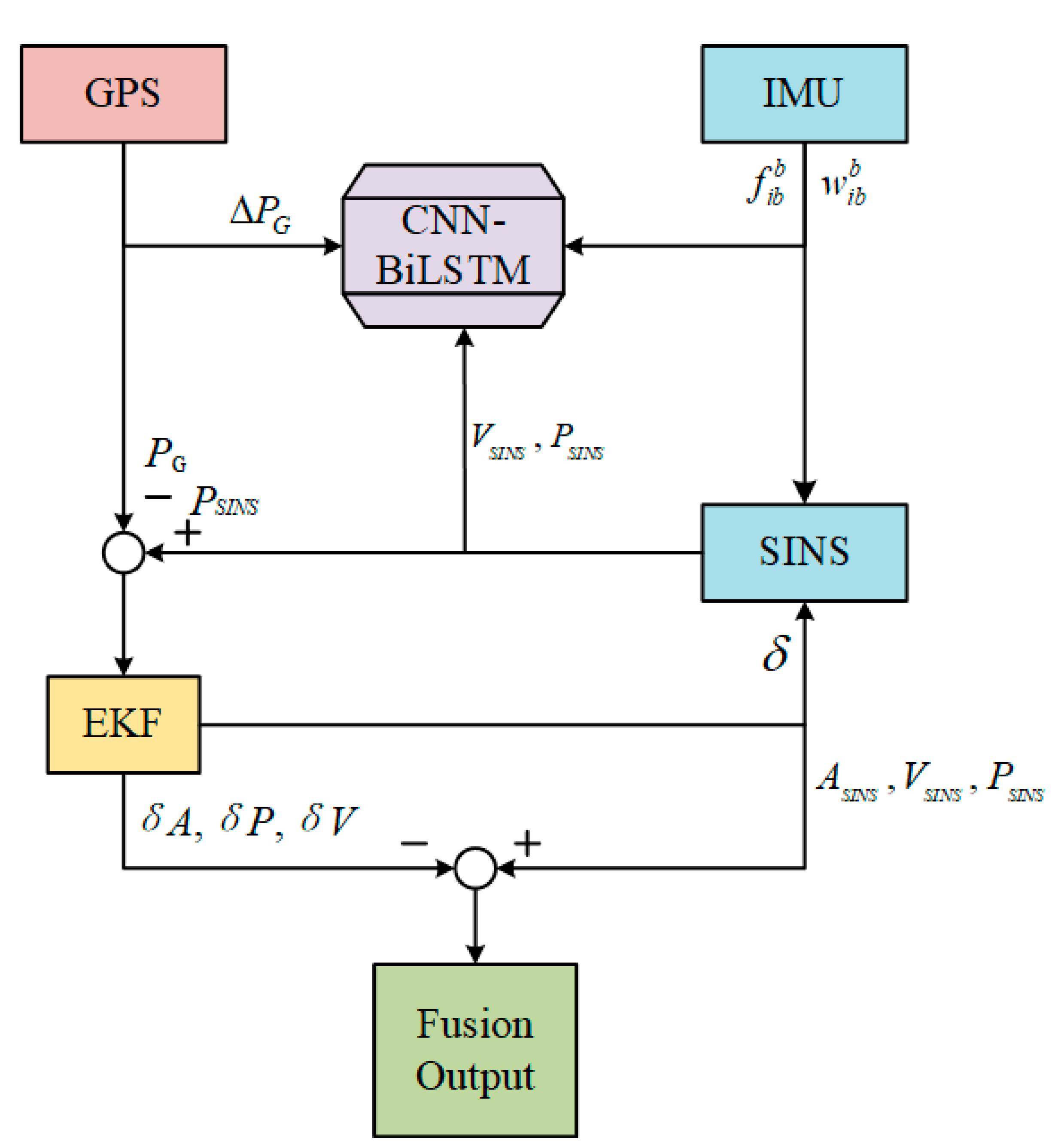
3.4. CNN—BiLSTM Neural Network-Assisted GNSS/INS Integrated Navigation System Model

In the neural network training model, selecting input and output features is a fundamental step in constructing a neural network to assist GNSS/INS integrated navigation. The input features consist of three-axis angular velocity and specific force data provided by the IMU, along with the position and velocity information derived from SINS computations. The output features, serving as labels, are typically the INS navigation errors, including position errors, velocity errors, and attitude errors. Theoretically, the output features should include position increments, velocity increments, and misalignment angle increments, encompassing a total of nine dimensions. However, using excessively high-dimensional output features can degrade the training performance of the model.

Considering the practical scenario of tractor farming operations, where there is minimal variation in altitude, users are primarily concerned with horizontal positional deviations that may cause the tractor to veer off the designated route or farmland. Additionally, the RTK-GPS used in this study provides centimeter-level positioning accuracy.Therefore, the output features, serving as target values for training the model, are selected as the latitude and longitude increments derived from the RTK-GPS output. This reduction in the dimensionality of output features enhances the model's effectiveness.

The neural network model designed in this study to assist the integrated navigation system is primarily divided into two phases: the training phase and the prediction phase.

As illustrated in Figure 5, when the GNSS signal is normal, the differences between the GNSS and SINS outputs for position and velocity are computed and input into the integrated navigation filter for EKF data fusion. The outputs, $\delta P$ and $\delta V$, are fed back into the SINS for correction and subsequently used to update the SINS outputs for position and velocity, providing the final integrated navigation results. Simultaneously, the angular velocity and specific force measured by the IMU, along with the position and velocity computed by SINS, are used as inputs for neural network training. The position increments from DGPS serve as the desired output for training the CNN-BiLSTM neural network. The predicted output from the trained neural network is compared with the target values to calculate the network's loss function. Through extensive training and employing the gradient descent algorithm, the weights matrix is iteratively optimized until the loss function converges to its minimum value.

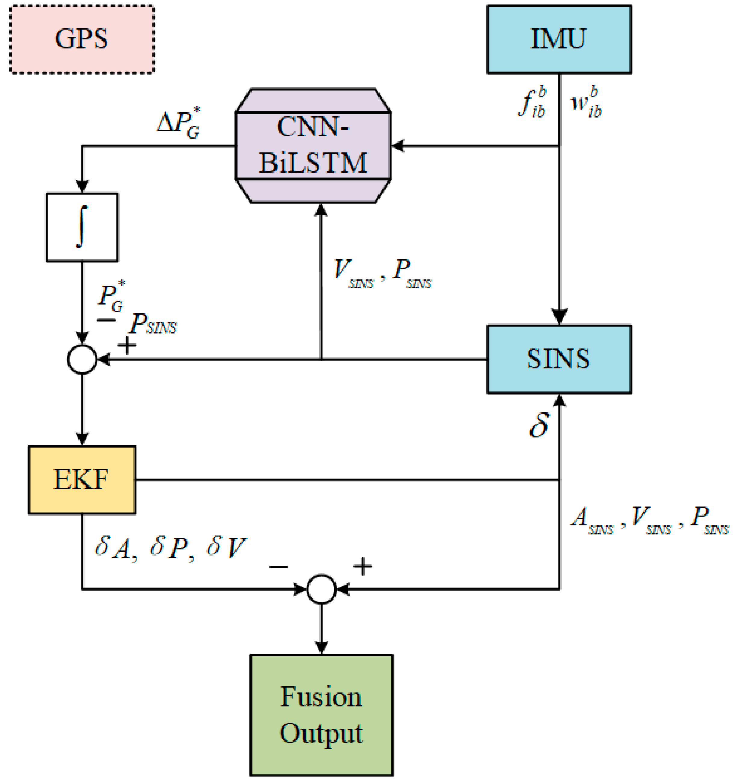
As depicted in Figure 6, when the GNSS signal is lost, the system transitions into the prediction phase. The outputs from the IMU and SINS continue to serve as inputs. The trained CNN-BiLSTM neural network model, equipped with the optimized weight matrix from prior training, is utilized to predict GPS position increments $\Delta P_G$. By integrating these increments, pseudo-GPS information is $P_{\ast }^G$ derived, which acts as a substitute reference for position information during the GNSS signal outage. This pseudo-GPS data is subsequently employed in the EKF measurement update to provide error corrections for the SINS-derived results, thereby producing the neural network-assisted integrated navigation output.

4. Experiment and Results Analysis

4.1. Experimental Equipment and Scenario

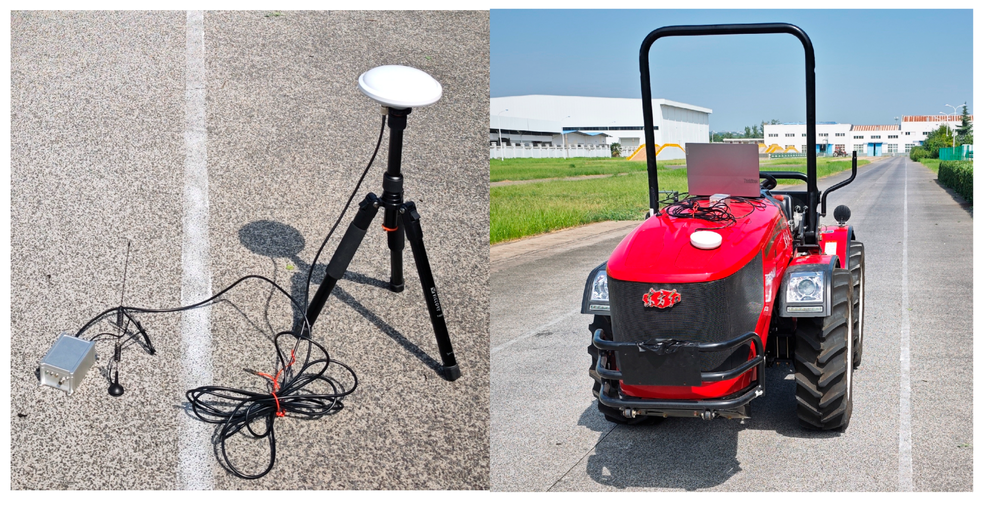
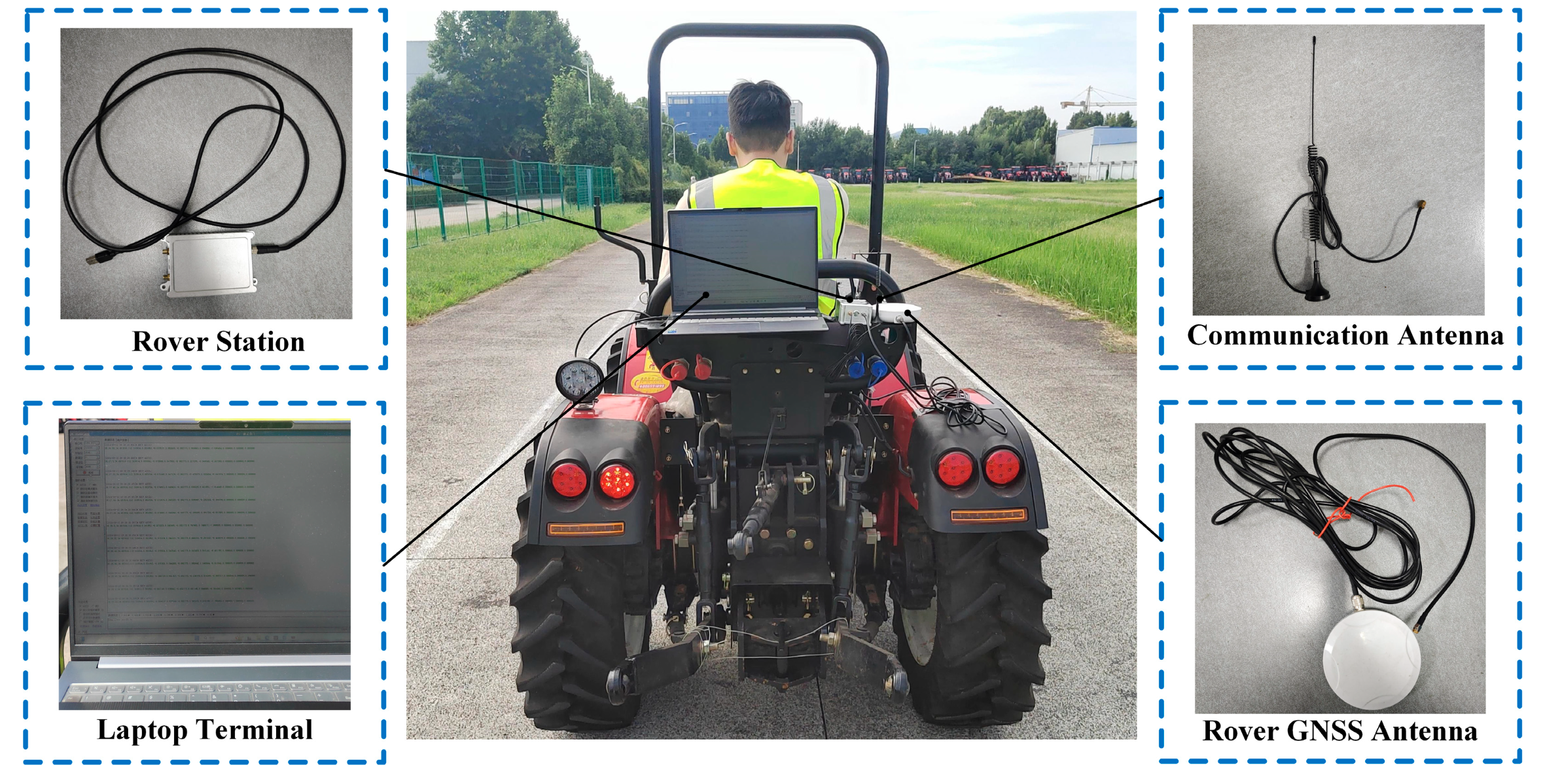
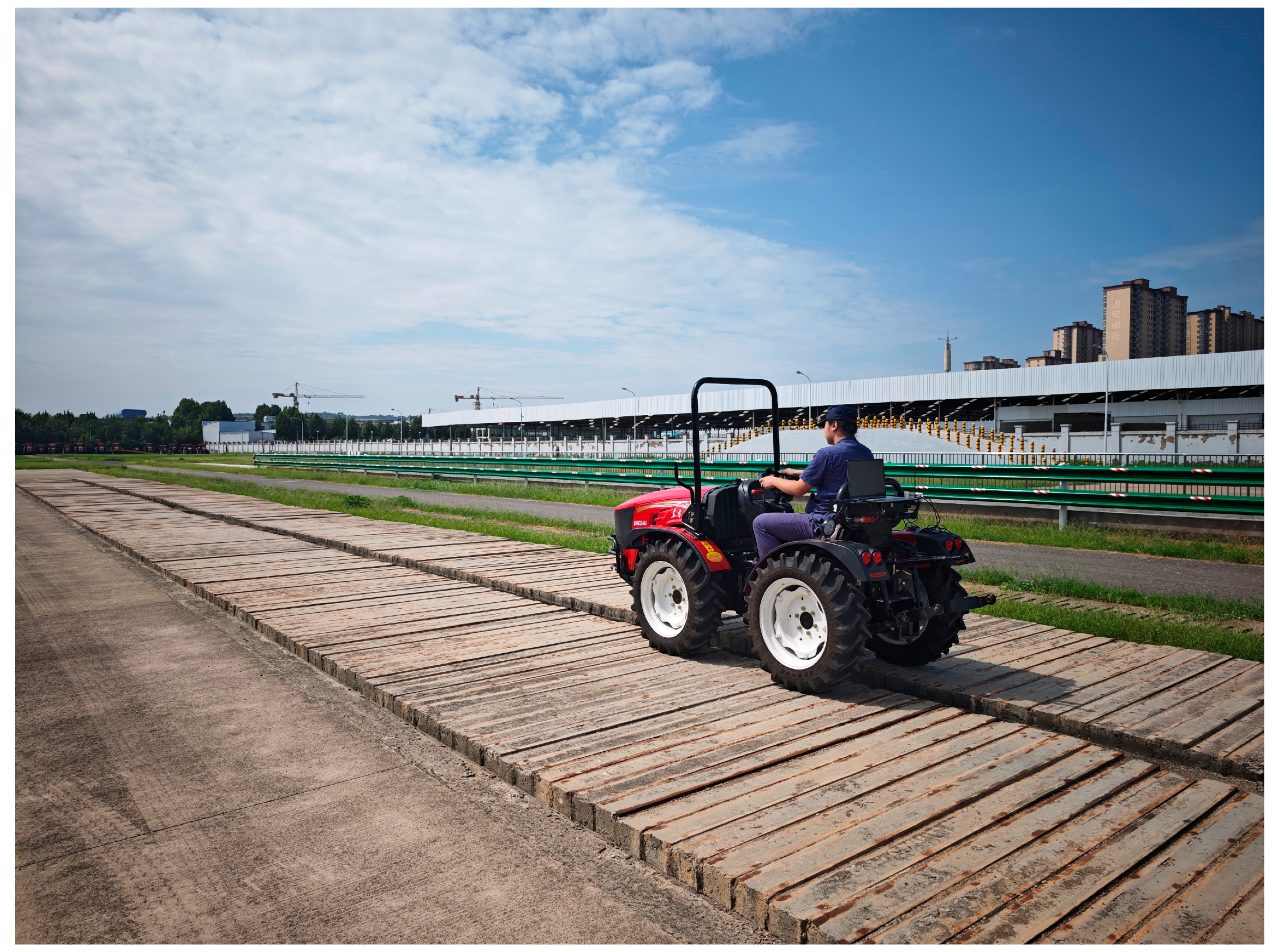
Directly collecting data in obstructed environments may lead to a decline in the accuracy of the reference solution, or even result in inaccuracies. Therefore, data is first collected in an open environment, followed by a simulated GPS failure to replicate the effects of obstruction, in order to assess the performance of the neural network-assisted GNSS/INS integrated navigation algorithm. The experimental data was gathered at the trial runway area of the China Yituo pilot base. The test site is an open-air, unobstructed field, and the data collection lasted approximately 24 minutes. The mobile integrated testing platform, as shown in the figure, consists of a self-developed inertial navigation system coupled with GPS, fixed on a certain model of Dongfanghong hilly tractor, along with a GNSS receiver and RTK base station.

The RTK reference station was placed near the runway, with a signal reception range of approximately 500 meters in radius. The mobile station was mounted on the tractor, with an installation diagram shown in Figure 8.

The tractor's field operation scenario was simulated on a rugged runway, as depicted in Figure 9.

During the experiment, the tractor was driven back and forth across rugged terrain to simulate field operations, collecting over 1400 seconds of real-time data. The data was pre-processed to remove gross errors, duplicates, and inaccuracies, before being used to train the CNN-BiLSTM model. The data was divided into training and validation sets in a 4:1 ratio, with a GPS failure simulated between 500 and 600 seconds. Root Mean Square Error (RMSE) was used as the evaluation metric.

4.2. Comparative Analysis During 100 Seconds of GNSS Signal Loss

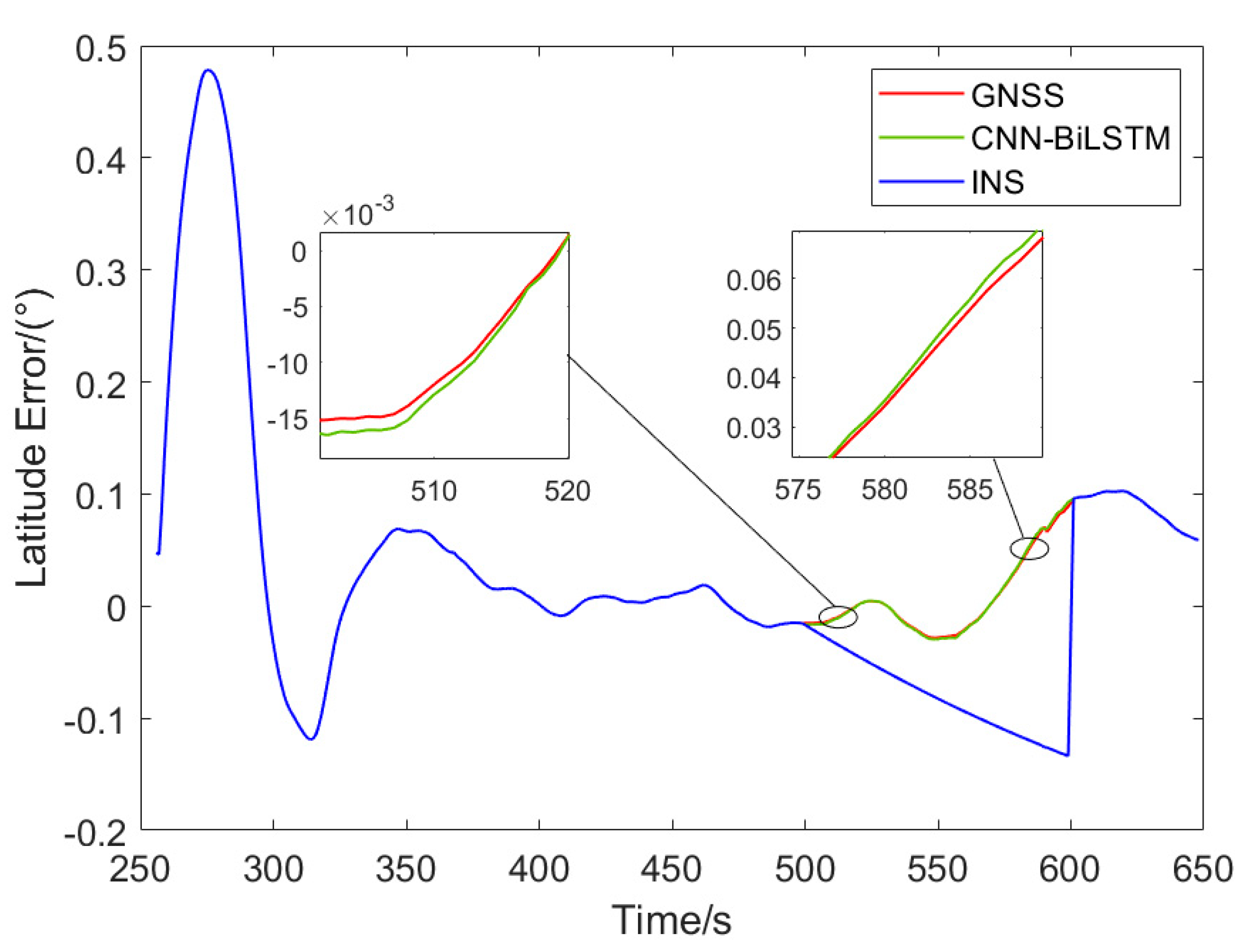
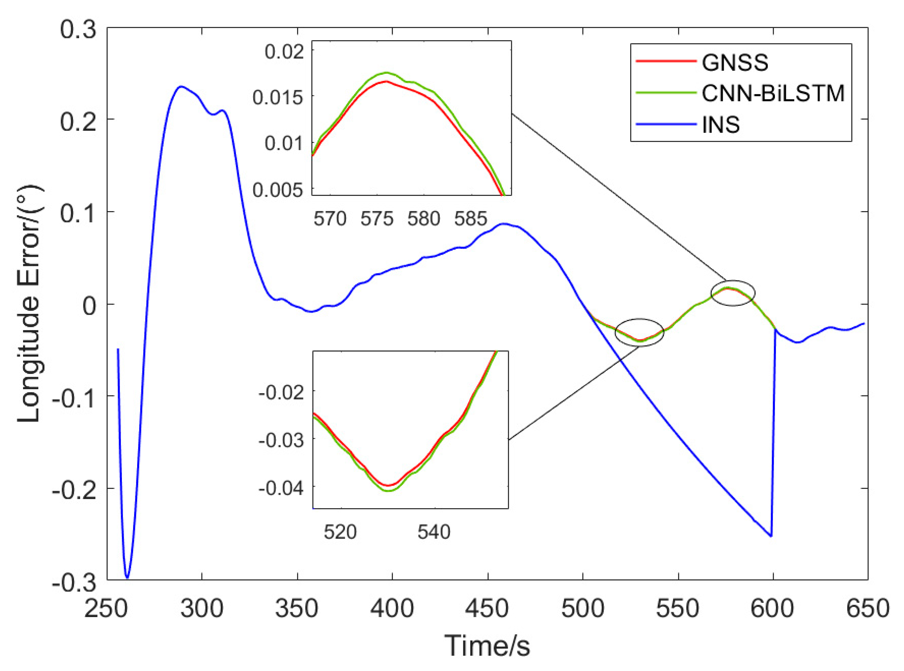
To better assess the performance of the proposed model, comparisons were made under three scenarios: GPS functioning normally, GPS failure with CNN-BiLSTM-assisted integrated navigation, and pure inertial navigation (INS) without any model assistance. Since the tractor's altitude remained relatively stable during field operations, Figure 9 and Figure 10 illustrate the errors in latitude and longitude position information after the Kalman filtering process for all three conditions.

From Figure 10 and Figure 11, and Table 1, it can be observed that during the 100 seconds of GPS signal loss, the absence of GPS location information causes a significant accumulation of errors in the pure inertial navigation solution. In contrast, the neural network model, compared to the pure inertial navigation (INS) solution, significantly reduces the error. A closer comparison between the model predictions and the actual GPS data reveals that the CNN-BiLSTM model achieves high accuracy in predicting latitude and longitude information.

This result demonstrates that our neural network model can effectively replace GPS for updating position information during periods of GPS signal loss, confirming its potential for enhancing the robustness of GNSS/INS integrated navigation systems in obstructed environments.

As shown in Table 1, during the 100-second period of GPS failure, the average absolute errors (MAE) in longitude and latitude obtained using the CNN-BiLSTM model to replace GPS-assisted INS calculations are 0.0195° and 0.0244°, respectively. In contrast, the MAEs for the pure inertial navigation system (INS) are 0.1345° and 0.0784°, reflecting a reduction of 85.5% and 68.9% in MAE, respectively. Similarly, the root mean square errors (RMSE) for the CNN-BiLSTM-based calculations are 0.0230° and 0.0340° for longitude and latitude, while the RMSE for pure INS are 0.1529° and 0.0853°, showing a reduction of 85% and 60.1% in RMSE, respectively. These results demonstrate that the model-assisted integrated navigation significantly reduces the positional errors in INS calculations.

Compared to the GPS-derived results, the MAE for GPS longitude and latitude are 0.0189° and 0.0234°, while the CNN-BiLSTM-derived MAE are 0.0195° and 0.0244°, respectively, showing increases of 3.2% and 4.3% in MAE for the latter. Similarly, the RMSE for GPS longitude and latitude are 0.0223° and 0.0327°, while the RMSE for CNN-BiLSTM are 0.0230° and 0.0340°, showing increases of 3.1% and 4% for the latter, indicating that the model's fitting accuracy is notably high. Overall, whether for longitude or latitude information, the CNN-BiLSTM model outperforms the pure INS system and exhibits a fitting accuracy comparable to that of the GPS-derived results.

5. Conclusions

This paper addresses the challenges faced by autonomous tractors in field operations, specifically the loss or interference of GNSS signals. We propose a CNN-BiLSTM-assisted GNSS/INS integrated navigation algorithm. When GNSS signals are available, the model is trained using the outputs from the IMU and SINS, with RTK-GPS data serving as the reference. In the event of GNSS signal loss, the trained CNN-BiLSTM model is utilized to predict the tractor's longitude and latitude, thereby preventing significant errors that could arise from pure INS calculations, which would otherwise compromise the navigation accuracy during field operations. The predicted results are then compared with the GNSS outputs during normal operation to assess the model's fitting performance.

Through experimental data simulating tractor field operations, we trained our model and applied a MATLAB simulation of a 100-second GPS outage. When GPS was unavailable for 100 seconds, the proposed neural network-assisted integrated navigation system significantly outperformed pure INS-based navigation: the average absolute error in longitude decreased by 85.5%, the root mean square error by 85%, the average absolute error in latitude dropped by 68.9%, and the root mean square error by 60.1%. Furthermore, when compared to actual GPS data, both the average absolute error and the root mean square error for latitude and longitude did not exceed 4%. The experimental results confirm that the algorithm proposed in this paper can effectively mitigate the cumulative errors in integrated navigation positioning during GNSS signal loss. Additionally, its fitting performance is comparable to that of GNSS, enabling the enhancement of tractor operation efficiency and accuracy even in complex environments where GNSS signals are denied.

References

- Yue, G.; Pan, Y. Intelligent Control System of Agricultural Unmanned Tractor Tillage Trajectory. J. Intell. Fuzzy Syst. 2020, 38, 7449–7459. [Google Scholar] [CrossRef]
- Karunathilake, E.M.B.M.; Le, A.T.; Heo, S.; Chung, Y.S.; Mansoor, S. The Path to Smart Farming: Innovations and Opportunities in Precision Agriculture. Agriculture-Basel 2023, 13, 1593. [Google Scholar] [CrossRef]
- Wan, M.; Liu, D.; Wu, J.; Li, L.; Peng, Z.; Liu, Z. State Estimation for Quadruped Robots on Non-Stationary Terrain via Invariant Extended Kalman Filter and Disturbance Observer. Sensors 2024, 24, 7290. [Google Scholar] [CrossRef]
- Fan, X.; Wang, J.; Wang, H.; Yang, L.; Xia, C. LQR Trajectory Tracking Control of Unmanned Wheeled Tractor Based on Improved Quantum Genetic Algorithm. Machines 2023, 11, 62. [Google Scholar] [CrossRef]
- Lan, L.I.; Feng, Z.H.U.; Wanke, L.I.U.; Xiaohong, Z. GNSS Pseudorange Stochastic Model for Urban Classification Scenes and Its Positioning Performance. whdxxbxxkxb 2023. [Google Scholar] [CrossRef]
- Hanxu, L.I.; Xin, L.I.; Guanwen, H.; Qin, Z.; Shipeng, C. LSTM Neural Network Assisted GNSS/SINS Vehicle Positioning Based on Speed Classification. whdxxbxxkxb 2024. [Google Scholar] [CrossRef]
- Chen, K.; Chang, G.; Chen, C. GINav: A MATLAB-Based Software for the Data Processing and Analysis of a GNSS/INS Integrated Navigation System. GPS Solut 2021, 25, 108. [Google Scholar] [CrossRef]
- Yin, Z.; Mengqi, X.; Hongliang, Y. Design of the GNSS/INS integrated navigation system for intelligent agricultural machinery. nygcxb 2021, 37, 40–46. [Google Scholar] [CrossRef]
- Zhuang, Y.; Sun, X.; Li, Y.; Huai, J.; Hua, L.; Yang, X.; Cao, X.; Zhang, P.; Cao, Y.; Qi, L.; et al. Multi-Sensor Integrated Navigation/Positioning Systems Using Data Fusion: From Analytics-Based to Learning-Based Approaches. Inf. Fusion 2023, 95, 62–90. [Google Scholar] [CrossRef]
- Liu, P.; Wang, B.; Li, G.; Hou, D.; Zhu, Z.; Wang, Z. SINS/DVL Integrated Navigation Method With Current Compensation Using RBF Neural Network. IEEE Sens. J. 2022, 22, 14366–14377. [Google Scholar] [CrossRef]
- Ning, Y.; Wang, J.; Han, H.; Tan, X.; Liu, T. An Optimal Radial Basis Function Neural Network Enhanced Adaptive Robust Kalman Filter for GNSS/INS Integrated Systems in Complex Urban Areas. Sensors 2018, 18, 3091. [Google Scholar] [CrossRef] [PubMed]
- Chen, L.; Fang, J. A Hybrid Prediction Method for Bridging GPS Outages in High-Precision POS Application. IEEE Trans. Instrum. Meas. 2014, 63, 1656–1665. [Google Scholar] [CrossRef]
- Ebrahimi, A.; Nezhadshahbodaghi, M.; Mosavi, M.R.; Ayatollahi, A. An Improved GPS/INS Integration Based on EKF and AI During GPS Outages. J. Circuits Syst. Comput. 2024, 33, 2450035. [Google Scholar] [CrossRef]
- Xu, Y.; Wang, K.; Yang, C.; Li, Z.; Zhou, F.; Liu, D. GNSS/INS/OD/NHC Adaptive Integrated Navigation Method Considering the Vehicle Motion State. IEEE Sens. J. 2023, 23, 13511–13523. [Google Scholar] [CrossRef]
- Xu, Y.; Wang, K.; Jiang, C.; Li, Z.; Yang, C.; Liu, D.; Zhang, H. Motion-Constrained GNSS/INS Integrated Navigation Method Based on BP Neural Network. Remote Sens. 2023, 15, 154. [Google Scholar] [CrossRef]
- Wang, G.; Xu, X.; Yao, Y.; Tong, J. A Novel BPNN-Based Method to Overcome the GPS Outages for INS/GPS System. IEEE Access 2019, 7, 82134–82143. [Google Scholar] [CrossRef]
- Dai, H.; Bian, H.; Wang, R.; Ma, H. An INS/GNSS Integrated Navigation in GNSS Denied Environment Using Recurrent Neural Network. Def. Technol. 2020, 16, 334–340. [Google Scholar] [CrossRef]
- Fang, W.; Jiang, J.; Lu, S.; Gong, Y.; Tao, Y.; Tang, Y.; Yan, P.; Luo, H.; Liu, J. A LSTM Algorithm Estimating Pseudo Measurements for Aiding INS during GNSS Signal Outages. Remote Sensing 2020, 12, 256. [Google Scholar] [CrossRef]
- Lv, P.-F.; Lv, J.-Y.; Hong, Z.-C.; Xu, L.-X. Integration of Deep Sequence Learning-Based Virtual GPS Model and EKF for AUV Navigation. Drones 2024, 8, 441. [Google Scholar] [CrossRef]
- Tao, L.; Zhang, P.; Gao, K.; Liu, J. Global Navigation Satellite System/Inertial Measurement Unit/Camera/HD Map Integrated Localization for Autonomous Vehicles in Challenging Urban Tunnel Scenarios. Remote Sensing 2024, 16, 2230. [Google Scholar] [CrossRef]
- Falco, G.; Pini, M.; Marucco, G. Loose and Tight GNSS/INS Integrations: Comparison of Performance Assessed in Real Urban Scenarios. Sensors 2017, 17. [Google Scholar] [CrossRef] [PubMed]
- Chen, S.; Xin, M.; Yang, F.; Zhang, X.; Liu, J.; Ren, G.; Kong, S. Error Compensation Method of GNSS/INS Integrated Navigation System Based on AT-LSTM During GNSS Outages. IEEE Sens. J. 2024, 24, 20188–20199. [Google Scholar] [CrossRef]
- Song, L.; Xu, P.; He, X.; Li, Y.; Hou, J.; Feng, H. Improved LSTM Neural Network-Assisted Combined Vehicle-Mounted GNSS/SINS Navigation and Positioning Algorithm. Electronics 2023, 12, 3726. [Google Scholar] [CrossRef]
- Li, W.; Lian, Y.; Liu, Y.; Shi, G. Ship Trajectory Prediction Model Based on Improved Bi-LSTM. ASCE-ASME J. Risk. Uncertain. Eng. Syst. Part A.-Civ. Eng. 2024, 10, 04024033. [Google Scholar] [CrossRef]
- Hu, X.; Zhang, B.; Tang, G. Research on Ship Motion Prediction Algorithm Based on Dual-Pass Long Short-Term Memory Neural Network. IEEE Access 2021, 9, 28429–28438. [Google Scholar] [CrossRef]
- Chen, K.; Zhang, P.; You, L.; Sun, J. Research on Kalman Filter Fusion Navigation Algorithm Assisted by CNN-LSTM Neural Network. Appl. Sci.-Basel 2024, 14, 5493. [Google Scholar] [CrossRef]
- Zhi, Z.; Liu, D.; Liu, L. A Performance Compensation Method for GPS/INS Integrated Navigation System Based on CNN-LSTM during GPS Outages. Measurement 2022, 188, 110516. [Google Scholar] [CrossRef]
- Liu, N.; Hui, Z.; Su, Z.; Qiao, L.; Dong, Y. Integrated Navigation on Vehicle Based on Low-Cost SINS/GNSS Using Deep Learning. Wirel. Pers. Commun. 2022, 126, 2043–2064. [Google Scholar] [CrossRef]