Submitted:
19 November 2024
Posted:
20 November 2024
You are already at the latest version
Abstract
Investment return realizations often provide only partial distributional information, yet traditional portfolio optimization frameworks assume preserved statistical properties which can lead to modeling risk. To address this, we employ a robust optimization framework called Wasserstein distributionally robust optimization (WDRO) on the mean absolute deviation (MAD) of portfolio returns. This approach provides cross-distributional robustness via worst-case risk minimization over all distributions within a Wasserstein ball of radius ϵ centered on some empirical distribution estimate. However, as the number of assets increases, the optimization problem becomes high-dimensional and sensitive to signal noise. To alleviate this burden, we discard redundant assets from the investment universe by virtue of correlation market graph sparsification. To the best of our knowledge, the combination of market graph sparsification with the WDRO framework is a novel contribution introduced in this study. We demonstrate that this methodology delivers superior results in both computational efficiency and test-set return statistics when applied to real-world S&P500 stock price data from 2018 to 2024.
Keywords:
Financial signal processing
; Market graphs
; Sparsification
; Portfolio optimization
; Distributionally robust optimization
1. Introduction
An investment portfolio is a collection of distinct assets, represented analytically as a vector whose entries correspond to the percentage of total wealth allocated to each asset. To avoid the risks associated with leverage and short-selling, we constrain them in and further demand that they sum up to one (i.e. ), satisfying the budget constraint. For every asset , there exists a discrete-time stochastic process that generates closing price data at the end of day . Hence, we can define the daily return process of the asset as
Returns data has been widely adopted in the field and is generally preferred over raw price data as it typically exhibits stronger Gaussianity and serves as a metric for asset and portfolio performance [1].
A general portfolio optimization problem can be formulated as
where the function maps a portfolio to a real number representing the investment risk, and is parameterized by the N-variate returns process over all portfolio assets. Note that we have also compressed the weight constraints using set notation implying that, if , then the allocation is agnostic to short selling and loans, and the budget constraint is met.
1.1. Minimum Variance Portfolio
When it comes to risk, there is no universally accepted method for quantifying it, with the choice of model often driven by complexity, robustness, or even interpretability. In 1952, H. Markowitz [2] pioneered in measuring investment risk using the mean and covariance of asset returns, which became the de-facto standard in diversification practices.
By further imposing a constraint on eq. 2 such that the portfolio expected return meets or exceeds a desirable target we obtain the minimum variance (MV) optimization problem as shown below
where the cost function is quadratic with respect to the decision variable . Under this framework, the investor is responsible for choosing appropriate estimators for both the expected returns and returns covariance .
The Markowitz portfolio model performs best when return distributions are not significantly skewed. However, its practical reliability is compromised due to its sensitivity to estimates of the first and second-order moments [3]. Recognizing this limitation, Markowitz himself suggested incorporating factor models to estimate the covariance matrix, particularly for large portfolios where historical data may be insufficient or unreliable [4]. These shortcomings naturally led investors to seek alternative risk metrics.
1.2. Mean Absolute Deviation Portfolio
In 1991, H. Konno and H. Yamazaki [5] proposed the use of the mean absolute deviation of portfolio returns as an alternative. They tested their work on historical data from stocks within the Japanese NIKKEI225 and TOPIX indices demonstrating that under their framework the optimization problem is more robust. This was mainly attributed to the absence of the squaring effect due to the quadratic cost in the MV problem. The MAD optimization problem was formulated as
where the authors arbitrarily imposed that the expected asset returns be estimated via the historical sample average, suggesting that
Note that we deliberately dropped the tilde symbol to indicate realisations of returns within a specified timeframe of samples. They also defined a term
to compactly re-phrase eq. 4 as
The authors proceed to tractably formulate the optimisation problem in eq. 4 by splitting the absolute value and introducing auxiliary variables for every sample in the timeframe. The tractable formulation for the MAD optimisation problem thus becomes
Konno and Yamazaki [5] also emphasize that, in contrast to the Markowitz portfolio, this involves solving a Linear Program (LP) with constraints regardless of investment universe size.
Comparative analyses have shown that the MAD model is more efficient and robust than the MV model. G. Kasenbacher et al. [6] demonstrated that the MAD model solves portfolio optimization problems involving over 1,000 stocks much faster than the MV model by avoiding the Quadratic Programming (QP) and covariance matrix inversions required. Additionally, Y. Simaan [7] argues that the MAD model offers a more conservative measure of risk by prioritizing the spread of portfolio returns from their expected value rather than focusing solely on return variance.
While there is extensive literature on alternative risk measures, such as Keating and Shadwick’s Omega function [8] which considers higher-order moments of the returns distribution. Our primary focus, however, will be on evaluating the performance of the MAD risk metric, particularly its distributionally robust counterpart called DRMAD as proposed by D. Chen et al. [9].
2. Distributional Robustness
In real-world optimization problems, particularly in portfolio optimization, a significant challenge arises from the uncertainty in estimating parameters, as data often fails to capture the joint density governing its stochasticity, even at the first and second-order moment level [10]. This uncertainty necessitates a robust optimization framework that avoids strict assumptions about the underlying parameter distribution. Distributionally robust optimization (DRO) offers such a solution by adopting a min-max approach, where the optimization problem is framed as a game between two players [11].
In this game, one player (the minimiser) seeks to optimize the portfolio under the worst-case scenario, while the other player (the maximizer) finds this scenario by searching for the probability distribution—within an ambiguity set —that maximizes the expected cost. Unlike traditional robust optimization (RO), which focuses on worst-case parameter realizations within a predetermined uncertainty set U [12], DRO achieves robustness by considering the worst-case distribution itself, based on partial distributional information such as moments, support, or even distributional proximity [13]. DRO improves model conservatism and robustness against parameter uncertainty by immunizing against the worst possible data-generating distribution, rather than just the worst parameter realization, making it a valuable tool in uncertain environments.
Distributionally Robust Mean Absolute Deviation Portfolio
In 2023, Chen et al. [9] introduced a novel portfolio optimization method called DRMAD by combining the MAD model with DRO which was shown to yield superior performance in fluctuating markets as compared to classical models. In our study, their work sets the foundation with which we explore the robustness and performance of our graph-theoretic sparsification framework. According to the work of D. Chen et al. [9] the DRMAD portfolio optimization problem is defined as
In contrast to the regular MAD problem defined in eq. 4, the distributionally robust mean absolute deviation (DRMAD) model incorporates a level of conservatism by framing the optimization task as a two-player game in which the ambiguity set, denoted as , is a ball that contains all distributions that are in close proximity to a distribution estimate.
To contextualise this ball-like ambiguity set, consider a finite set of realisations of the returns vector over a timeframe of T samples. We can estimate the unknown returns distribution using a non-parametric empirical estimate defined as
where is a Dirac measure concentrated at the point . It is reasonable to assume that the true distribution is "close" to its empirical estimate [9]. To formalise this notion of proximity, we introduce distance measures in the distribution space such as the Wasserstein distance [14].
Specificlly, given two probability distributions and on the same space , with representing the set of distributions supported on , their Wasserstein distance of order 1, denoted as , is defined as
where the coupling is a joint distribution on whose marginals are and , and is an arbitrary distance metric on the space of outcomes. Following the approach in [9], we adopt the norm as our distance function, i.e. . This allows us to define a Wasserstein ball in the distribution space which engulfs all distributions that are within a distance away from the empirical distribution . As a result the Wasserstein ambiguity set within the DRMAD formulation can be analytically defined as
As suggested by D. Kuhn and P. M. Esfahani [15,16], it is important to choose the radius hyperparameter carefully to balance robustness and computational feasibility, ensuring the solution remains tractable. We also note that the radius of this ball can be determined by other metrics, such as the Kullback-Leibler divergence [17].
The DRMAD portfolio optimization problem in eq. 9 is mathematically intractable because it is formulated as an infinite-dimensional non-convex optimization problem [18]. This arises from the Wasserstein ambiguity set, where the inner maximization is performed over a distribution in an infinite-dimensional space. To overcome this challenge, D. Chen et al. [9] propose a tractable reformulation by fixing the expected portfolio value as a decision variable, which transforms the problem into a finite-dimensional convex optimization problem [9]. This reformulation results in two Linear Programs (LPs), with the optimal solution corresponding to the portfolio weights derived from the program that yields the minimum cost. According to their work, these two LPs are
where represents the portfolio weights, is the sample average of the observed returns vector over a historical time window of T samples, and are auxiliary variables for each sample. Additionally, once again represents the investor’s target returns, while the ball radius can be interpreted as the risk appetite.
In the context of portfolio optimization, the investment universe dimension N emerges as a critical parameter. The inclusion of assets that contribute minimally or redundantly to the portfolio would complicate the optimization process by increasing the dimension of the Wasserstein ball. This would burden the search for the worst-case distribution, and would introduce unnecessary noise into the system. Additionally, a high portfolio dimensionality results in individual portfolio weights that are often too small to be of practical significance. Therefore, even though the DRMAD framework remains tractable under a large number of assets [9], it is advantageous to methodically reduce the problem dimensionality without sacrificing robustness.
3. Market Graphs
To address the inherent challenges associated with excessive portfolio dimensionality, we propose a graph-theoretic framework that sparsifies the structure of correlation market graphs, in which nodes represent assets and the edges connecting them capture historical return data correlations. This approach systematically eliminates redundant assets by reducing graph density, enabling the optimization of DRMAD portfolios within a reduced investment universe. Furthermore, this framework provides interpretability in the asset selection process prior to optimization via market graph visuals. Despite the demonstrated potential of distributionally robust optimization [9,19] and graph theory [20,21,22] in financial applications, their combined application remains unexplored in the literature. This study endeavors to fill this gap by introducing the integration of market graphs and sparsification into the DRMAD framework.
Traditionally, graphs are denoted as bold capitalised calligraphic characters, such as and . A set of sets is also a set and follows the same notation. Working with set notation to represent graphs, however, becomes increasingly cumbersome as the number of nodes and connections grow. To manage this, linear algebra has been established as a ubiquitous mathematical framework for modeling and analyzing graph structures. Hence, vectors are still represented by bold lowercase letters (e.g., ), and matrices are denoted by bold uppercase letters (e.g., ).
In any graph, the interaction strengths between vertices u and v can be represented by scalar quantities . These edge weights can then be summarized in a so-called combination matrix , where N denotes the number of vertices, i.e. the cardinality of [23]. The spatial relationships among the vertices are naturally captured in the matrix structure by the arrangement of these weights. The combination matrix is formally constructed as
where indicates the interaction strength across vertices u and v.
This concise graph representation framework also allows for a logical inversion, where any square matrix can be interpreted as a graph structure, especially when its elements carry physical meaning. For example, consider a collection of N asset return realizations . The matrix , as shown in eq. 17 below, can be defined to contain the absolute correlation coefficients between all return pairs in which is the sample covariance.
Subsequently, takes the form
where we note that and by construction. To construct the correlation market graph, nodes representing assets are connected only if they are statistically correlated, with edges weighted according to the strength of this correlation. Figure 1 illustrates this using 9 randomly chosen stocks from the S&P500 index, where nodes are labeled by stock ticker symbols and edges are color-coded to qualitatively represent return data correlations.
Apart from aesthetic appeal, the market graph visual offers a geometrical interpretation of our data. For example, the strong connections between Microsoft (’MSFT’), Cisco (’CSCO’), and Intel (’INTC’) could reveal overlapping market factors such as industry, reinforcing the need for careful consideration of the investment universe prior to optimization.
Correlation graphs are typically complete, resulting in a quadratic increase in the number of edges as the number of nodes grow [23]. The maximum number of edges in an N-vertex complete graph is given by , and consequently, the combination matrix has no null entries, leading to market graph visuals that can become cluttered and difficult to interpret.
4. Sparsification
Graph sparsification is a process that approximates dense graphs by reducing the number of edges and nodes based on application-specific algorithms [24]. Several sparsification algorithms exist in the literature, each employing different methodologies. Zhang et. al [25] use Ricci curvature sparsification to reduce computational burden in graph neural networks (GNNs), whereas Ahmadinejad et. al [26], for example, employ a singular value approximation approach as an alternative to standard [27] (directed) graph approximations. To promote interpretability of the sparsification process, however, we employ a threshold-based sparsification algorithm on the correlation market graph as shown below.
| Algorithm 1 Sparsification of Market Graph |
|
Given some correlation matrix and a correlation threshold , the algorithm iterates over the upper triangular portion of . There is no need to iterate over every pair as the correlation matrix is symmetric by construction, i.e. . For each pair of assets, if the absolute correlation is less than or equal to the threshold , those assets are added to the set representing the new investment universe in which .
A visual demonstration of this sparsification algorithm is shown in Figure 2, where it has been applied on the market graph of the previous section for consistency. Moreover, we employ three correlation thresholds of 0.6, 0.4, and 0.2 to demonstrate the stock filtering capabilities of the algorithm. Note that, initially, the total number of stocks were 9, but after each sparsification procedure, only case (C) shows a reduced investment universe. In the two remaining cases the graphs were indeed sparsified but only at an edge level.
5. Numerical Example
To evaluate the performance of the DRMAD portfolio under the proposed graph sparsification scheme we used historical daily stock closing price data from the S&P500’s 100 most liquid stocks based on average trading volume. The dataset spans the period 31 DEC 2017 to 02 JAN 2024 but we split it into training and testing sets. The training data (31 DEC 2017 to 02 JAN 2019) was used to generate portfolio weights, whereas the testing dataset (02 JAN 2019 to 02 JAN 2024) was used to evaluate portfolio performance based mainly on the Sharpe ratio (SR), which in this study is defined as the ratio over the average portfolio returns to their standard deviation.
We implemented three DRMAD optimisers using the CVXPY package [28,29] with Wasserstein radii of 0, 0.1, and 1, respectively. Note that the portfolio weights from the 0 radius case are equivalent to those produced by a classic MAD portfolio as defined in eq. 8 [9]. Before deploying the optimisers, however, we also performed our graph sparsification method on the 100-asset correlation matrix using the threshold values of 0.001, 0.01, and 1. Trivially, when the correlation threshold was set to 1, the investment universe remained intact, consisting of all 100 stocks, but when using a threshold of 0.01 and 0.001 the number of assets under consideration were reduced to 32 and 9, respectively. It is common in the literature to also deploy the minimum variance (MV) portfolio (see eq. 3) whose investment universe will not be subject to sparsification. For consistency, all target returns were set to the asset-wide average training set return. Finally, we tracked the computational time needed to generate the portfolio weights under all DRMAD configurations in order to investigate the computational efficiency gain due to sparsification.
Subsequently, we applied the obtained portfolio weights to the test-set returns data spanning 5 years. To evaluate performance, we compared the growth of a $1 initial investment in each portfolio on top of the growth of the S&P500 index during the same period. Figure 3a–c display the accumulation of wealth, where each figure displays a set of DRMAD portfolios with common radius across different sparsification schemes. We also zoomed in the first six months of 2020 to observe the performance of our portfolios during unforeseen events like the breakout of the COVID-19 pandemic.
We immediately observe that all DRMAD portfolios perform the best when the Wasserstein radius is sufficiently large. In this example, a ball radius of 1 yields the best results. This can be attributed to the regularizing effect of the radius hyperparameter aiding in generalization by virtue of distributional robustness. In all of the cases however, irrespective of radius, we notice that the smaller sized DRMAD portfolios consistently outperform their full 100-stock counterparts. Indeed, there exists some correlation threshold which reduces the investment dimension without sacrificing generalization, in fact, improving it. The sparsification process should not be too intense since an investment universe that is too small could prove insufficient and potentially produce sub-optimal results.
We quantitatively summarize our findings in term of test-set return statistics and optimizer runtime on Table 1. Notice that with only 32 stocks (i.e. a third of our initial investment universe) we were able to obtain portfolios that offer higher Sharpe ratios (SR) than those with equal Wasserstein radius. The best portfolio obtained used said 32 stocks with a radius of 1 resulting in a Sharpe ratio (SR) of 0.062, surpassing the S&P500 index by 37.8% during the same 5-year period. Even with a radius of 0.1, the 32-stock portfolio achieves a superior Sharpe ratio compared to the 100-stock portfolio, even when the latter is allowed a radius ten times larger.
Finally, the best portfolio in this example highlighted with bold font on Table 1, required 75ms to compute, whereas the 100-stock equivalent needed more than triple the time.
6. Conclusions
Our study highlights the effectiveness of reducing the dimensionality of the Wasserstein DRMAD portfolio optimization method through a threshold-based sparsification procedure. By eliminating stocks with excessive statistical correlations in historical returns data, we significantly reduce the computational burden of subsequent optimization efforts and, more importantly, filter out unnecessary signal noise, thereby improving test-set generalization. Additionally, sparsifying the correlation market graph enhances robustness and promotes a faithful representation of data’s true stochastic nature, which is crucial in identifying the worst-case distribution within the Wasserstein ball centered on the empirical estimate. This novel framework, which couples DRO and sparsification, offers both visual and mathematical clarity in the decision-making process in a way that is resourceful and interpretable.
Funding
This research received no external funding
Institutional Review Board Statement
Not applicable.
Informed Consent Statement
Not applicable.
Data Availability Statement
All S&P500 index and constituent daily closing price data can be found at https://finance.yahoo.com/markets/stocks/most-active/.
Conflicts of Interest
The authors declare no conflicts of interest.
References
- Mandic, D. Lecture 3 - Time Series Analysis of Financial Data 2022.
- Markowitz, H. PORTFOLIO SELECTION. The Journal of Finance 1952, 7, 77–91. [Google Scholar]
- Cheung, W. Markowitz versus 1/N: How Sensitive Is Mean-Variance Portfolio Performance to Estimation Errors? *, 2023.
- Markowitz, H.M. Portfolio Selection: Efficient Diversification of Investments; Yale University Press, 1959.
- Konno, H.; Yamazaki, H. Mean-Absolute Deviation Portfolio Optimization Model and Its Applications to Tokyo Stock Market. Management Science 1991, 37, 519–531, Publisher: INFORMS. [Google Scholar] [CrossRef]
- Kasenbacher, G.; Lee, J.; Euchukanonchai, K. Mean-Variance vs. Mean-Absolute Deviation: A Performance Comparison of Portfolio Optimization Models. PhD thesis, 2017.
- Simaan, Y. Estimation Risk in Portfolio Selection: The Mean Variance Model versus the Mean Absolute Deviation Model. Management Science 1997, 43, 1437–1446, Publisher: INFORMS. [Google Scholar] [CrossRef]
- Shadwick, W. A Universal Performance Measure Con Keating. 2002.
- Chen, D.; Wu, Y.; Li, J.; Ding, X.; Chen, C. Distributionally robust mean-absolute deviation portfolio optimization using wasserstein metric. Journal of Global Optimization 2023, 87, 783–805. [Google Scholar] [CrossRef] [PubMed]
- Mota, P.P. Normality assumption for the log-return of the stock prices. Discussiones Mathematicae Probability and Statistics 2012, 32, 47. [Google Scholar] [CrossRef]
- Sniedovich, M. Wald’s Maximin model: a treasure in disguise! Journal of Risk Finance 2008, 9, 287–291. [Google Scholar] [CrossRef]
- Ben-Tal, A.; El Ghaoui, L.; Nemirovskiĭ, A.S. Robust optimization; Princeton series in applied mathematics; Princeton University Press: Princeton, 2009. [Google Scholar]
- Van Parys, B.P.G.; Esfahani, P.M.; Kuhn, D. From Data to Decisions: Distributionally Robust Optimization Is Optimal. Management Science 2021, 67, 3387–3402. [Google Scholar] [CrossRef]
- Villani, C. The Wasserstein distances. In Optimal Transport; Berger, M., Eckmann, B., De La Harpe, P., Hirzebruch, F., Hitchin, N., Hörmander, L., Kupiainen, A., Lebeau, G., Ratner, M., Serre, D., Sinai, Y.G., Sloane, N.J.A., Vershik, A.M., Waldschmidt, M., Eds.; Grundlehren der mathematischen Wissenschaften; Springer Berlin Heidelberg: Berlin, Heidelberg, 2009; Vol. 338, pp. 93–111. [Google Scholar]
- Esfahani, P.M.; Kuhn, D. Data-driven Distributionally Robust Optimization Using the Wasserstein Metric: Performance Guarantees and Tractable Reformulations, 2017.
- Mohajerin Esfahani, P.; Kuhn, D. Data-driven distributionally robust optimization using the Wasserstein metric: performance guarantees and tractable reformulations. Mathematical Programming 2018, 171, 115–166. [Google Scholar] [CrossRef]
- Joyce, J.M. Kullback-Leibler Divergence. In International Encyclopedia of Statistical Science; Lovric, M., Ed.; Springer Berlin Heidelberg: Berlin, Heidelberg, 2011; pp. 720–722. [Google Scholar]
- Ambrosio, L.; Gigli, N. Ambrosio, L.; Gigli, N. A User’s Guide to Optimal Transport. In Modelling and Optimisation of Flows on Networks: Cetraro, Italy 2009, Editors: Benedetto Piccoli, Michel Rascle; Ambrosio, L., Bressan, A., Helbing, D., Klar, A., Zuazua, E., Eds.; Springer: Berlin, Heidelberg, 2013; pp. 1–155. [Google Scholar]
- Blanchet, J.; Chen, L.; Zhou, X.Y. Distributionally Robust Mean-Variance Portfolio Selection with Wasserstein Distances, 2018.
- Ambiel, T.; Castilho, D.; de Carvalho, A.C.P.L.F. The Strength of Influence Ties in Stock Networks: Empirical Analysis for Portfolio Selection. 2023 IEEE International Conference on Data Mining Workshops (ICDMW), 2023, pp. 456–464. ISSN: 2375-9259.
- Dees, B.S.; Stankovic, L.; Constantinides, A.G.; Mandic, D.P. Portfolio Cuts: A Graph-Theoretic Framework to Diversification. ICASSP 2020 - 2020 IEEE International Conference on Acoustics, Speech and Signal Processing (ICASSP); IEEE: Barcelona, Spain, 2020; pp. 8454–8458. [Google Scholar]
- Cardoso, J.V.d.M.; Ying, J.; Palomar, D.P. Algorithms for Learning Graphs in Financial Markets, 2020.
- Stankovic, L.; Mandic, D.; Dakovic, M.; Brajovic, M.; Scalzo Dees, B.; Li, S.; Constantinides, A. Data Analytics on Graphs; 2020.
- Chen, Y.; Ye, H.; Vedula, S.; Bronstein, A.; Dreslinski, R.; Mudge, T.; Talati, N. Demystifying Graph Sparsification Algorithms in Graph Properties Preservation, 2023. Version Number: 1.
- Zhang, X.; Song, D.; Tao, D. Ricci Curvature-Based Graph Sparsification for Continual Graph Representation Learning. IEEE Transactions on Neural Networks and Learning Systems 2024, 1–13. [Google Scholar] [CrossRef] [PubMed]
- Ahmadinejad, A.; Peebles, J.; Pyne, E.; Sidford, A.; Vadhan, S. Singular Value Approximation and Sparsifying Random Walks on Directed Graphs. 2023 IEEE 64th Annual Symposium on Foundations of Computer Science (FOCS); IEEE: Santa Cruz, CA, USA, 2023; pp. 846–854.
- Cohen, M.B.; Kelner, J.; Peebles, J.; Peng, R.; Rao, A.B.; Sidford, A.; Vladu, A. Almost-linear-time algorithms for Markov chains and new spectral primitives for directed graphs. Proceedings of the 49th Annual ACM SIGACT Symposium on Theory of Computing; STOC 2017. Association for Computing Machinery: New York, NY, USA, 2017; pp. 410–419.
- Diamond, S.; Boyd, S. CVXPY: A Python-embedded modeling language for convex optimization. Journal of Machine Learning Research 2016, 17, 1–5. [Google Scholar]
- Agrawal, A.; Verschueren, R.; Diamond, S.; Boyd, S. A rewriting system for convex optimization problems. Journal of Control and Decision 2018, 5, 42–60. [Google Scholar] [CrossRef]
Figure 1.
Correlation market graph visual for 9 randomly selected S&P500 stocks. Edges represent the absolute correlation coefficients between pairs of distinct stock return time-series based on daily closing prices from 31 DEC 2017 until 02 JAN 2019 inclusive.
Figure 1.
Correlation market graph visual for 9 randomly selected S&P500 stocks. Edges represent the absolute correlation coefficients between pairs of distinct stock return time-series based on daily closing prices from 31 DEC 2017 until 02 JAN 2019 inclusive.
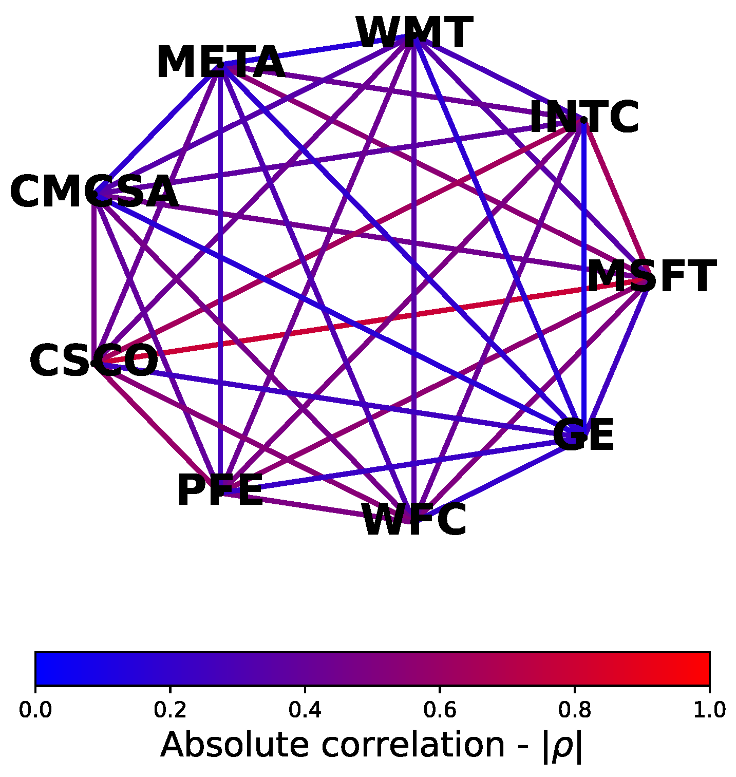
Figure 2.
Sparsified correlation market graph visuals with an initial 9 randomly selected S&P500 stocks. Edges represent the absolute correlation coefficients between pairs of distinct stock return time-series based on daily closing prices from 31 DEC 2017 up until 02 JAN 2019 inclusive. Example (A) shows edges for asset correlations of at most 0.6, whereas (B) and (C) show edges of correlations of at most 0.4 and 0.2, respectively. Only (C) shows a reduced investment universe.
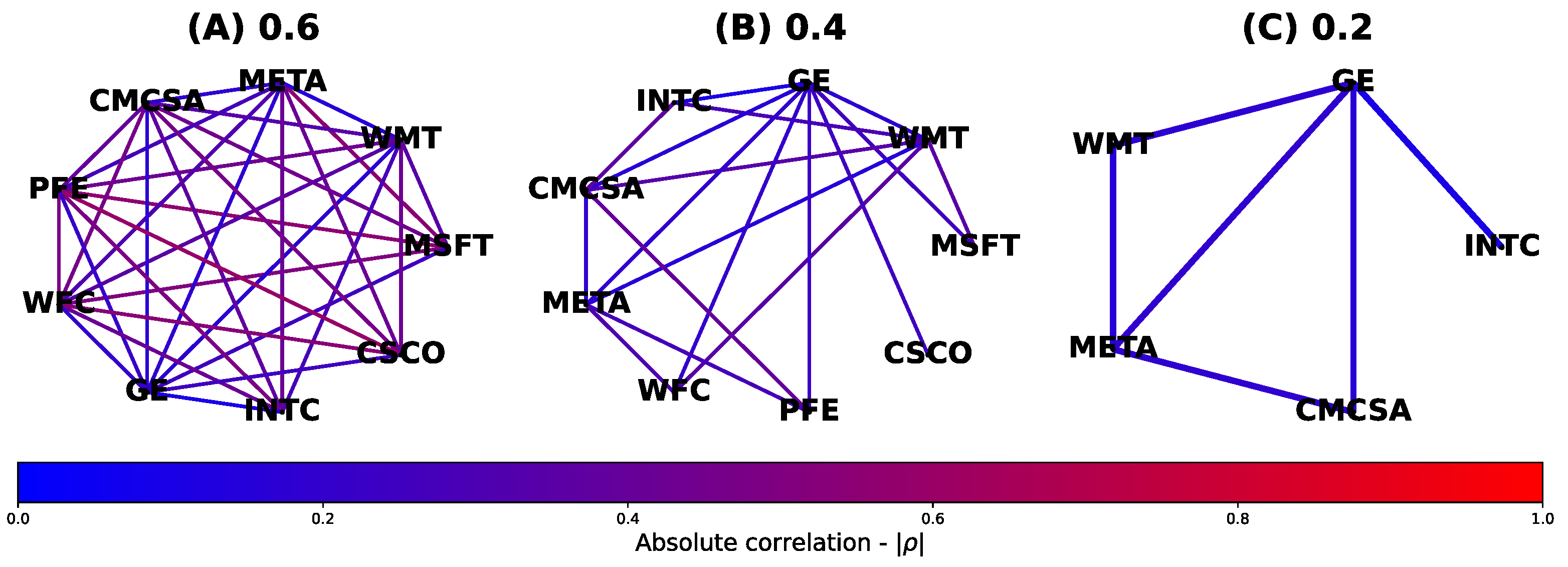
Figure 3.
Growth of a $1 investment placed in the S&P500 index, minimum variance, and distributionally robust mean absolute deviation (DRMAD) portfolios under various sparsification schemes of 0.001, 0.01 and 1 correlation thresholds yielding 9, 32, and 100 assets respectively. Target returns were set to the training set average return.
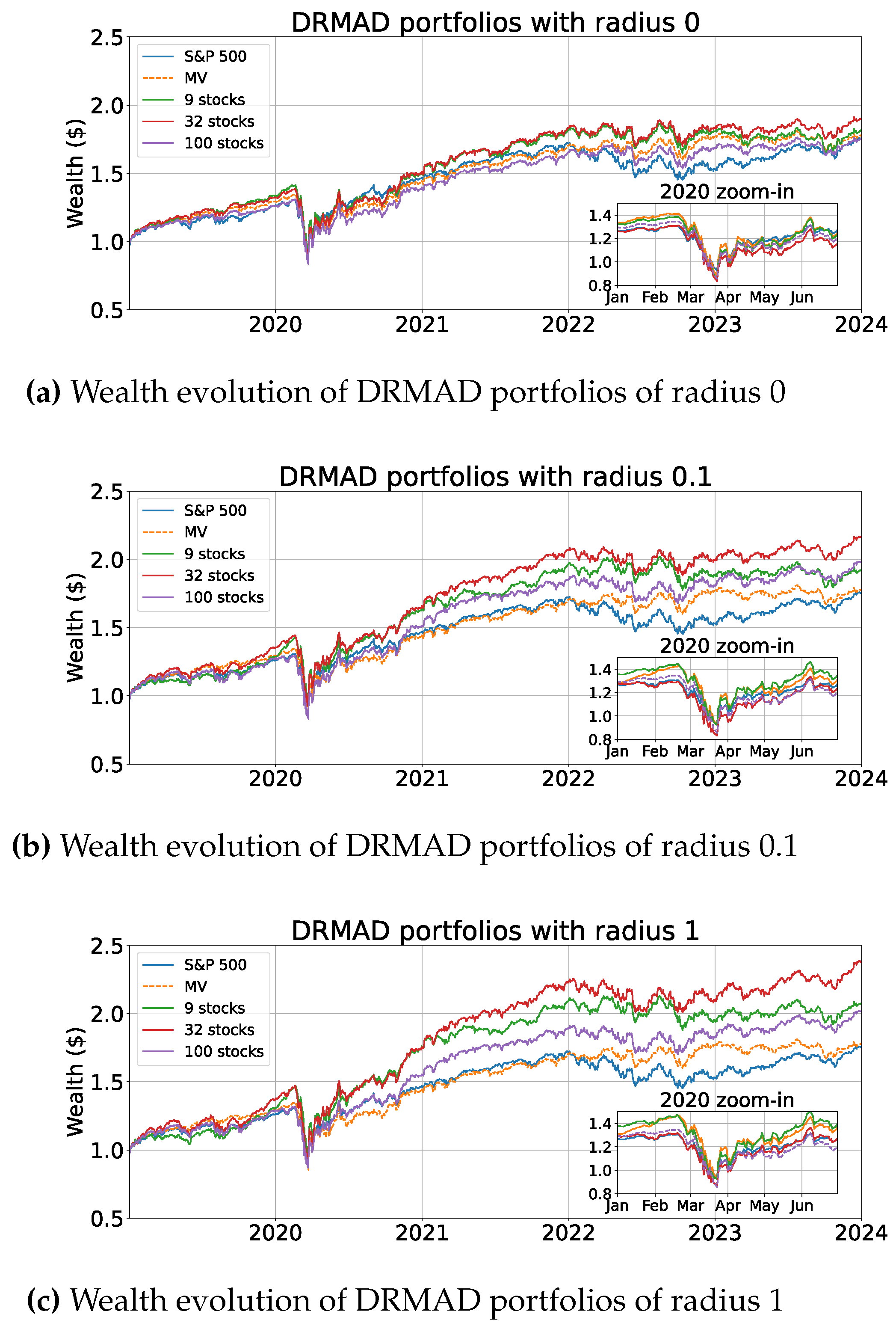

Table 1.
Test-set return statistics and optimizer computation time for the DRMAD portfolios under the proposed graph sparsification framework. Notice that there exists some threshold value resulting in superior Sharpe ratios (SR) across all radii values. The MV portfolio and the S&P500 index attained the Sharpe ratios of SRMV = 0.045, and SRS&P500 = 0.044, respectively.
| Threshold | Radius | Returns avg. (%) |
Returns stddev. |
SR | Runtime (ms) |
|---|---|---|---|---|---|
| 0.001 (9 assets) |
0 | 0.065 | 0.016 | 0.041 | 91 |
| 0.1 | 0.074 | 0.016 | 0.048 | 95 | |
| 1 | 0.086 | 0.016 | 0.053 | 52 | |
|
0.01 (32 assets) |
0 | 0.072 | 0.016 | 0.046 | 99 |
| 0.1 | 0.093 | 0.016 | 0.059 | 75 | |
| 1 | 0.109 | 0.018 | 0.062 | 75 | |
| 1 (100 assets) |
0 | 0.060 | 0.014 | 0.044 | 452 |
| 0.1 | 0.078 | 0.015 | 0.052 | 278 | |
| 1 | 0.081 | 0.015 | 0.054 | 267 |
Disclaimer/Publisher’s Note: The statements, opinions and data contained in all publications are solely those of the individual author(s) and contributor(s) and not of MDPI and/or the editor(s). MDPI and/or the editor(s) disclaim responsibility for any injury to people or property resulting from any ideas, methods, instructions or products referred to in the content. |
© 2024 by the author. Licensee MDPI, Basel, Switzerland. This article is an open access article distributed under the terms and conditions of the Creative Commons Attribution (CC BY) license (https://creativecommons.org/licenses/by/4.0/).
Copyright: This open access article is published under a Creative Commons CC BY 4.0 license, which permit the free download, distribution, and reuse, provided that the author and preprint are cited in any reuse.


