
Submitted:
19 November 2024
Posted:
20 November 2024
You are already at the latest version
Abstract
Estimating the amplitude of a sinewave from a set of data points is a common procedure in various applications. This is typically achieved using a least-squares method that provides closed-form estimators. The sampling process itself is often affected by different non-ideal phenomena like additive noise, phase noise or sampling jitter, for example. Here we study the precision of the estimation of a sinewave amplitude when the samples are affected by phase noise or sampling jitter. The mathematical expression derived is useful in obtaining the confidence intervals for the estimated sinusoidal amplitude. It is also valuable at the time of choosing the proper number of samples to acquire from a signal from which we need to estimate the sinusoidal amplitude in order to reach a certain desired level of estimation precision. The analytical expression presented is validated using both numerically generated data and experimental data. Various non-ideal factors, such as a fixed, uncontrollable amount of jitter in the setup, additive noise, analog-to-digital converter non-linearity, and limited signal bandwidth, are observed and discussed. Additionally, this work presents an exhaustive overview of the technical aspects involved in the experimental validation, including the implementation of the Monte Carlo type procedure, instrument interface, programming language, and the general development of automated measurement systems, which may be useful to other engineers.
Keywords:
least squares
; sine fitting
; amplitude estimation
; phase noise
; sampling jitter
1. Introduction
Estimating the amplitude of a sinewave from a set of data points is a fundamental task in numerous scientific and engineering applications, encompassing fields such as telecommunications, signal processing, and instrumentation. This process is crucial for analyzing and interpreting various phenomena accurately.
In mechanical engineering, monitoring the amplitude of mechanical vibrations is vital for predicting and preventing mechanical failures in engines, turbines, and other machinery [1]. By analyzing vibration amplitudes, engineers can identify early signs of wear and tear, thus implementing timely maintenance to avoid catastrophic failures. For instance, in predictive maintenance systems, vibration amplitude analysis is used to monitor the health of rotating machinery, ensuring optimal performance and longevity.
In seismology, estimating the amplitude of seismic waves is critical for assessing their magnitude and potential impact. Accurate amplitude measurements enable scientists to evaluate the energy released during an earthquake and predict the likely effects on buildings and infrastructure. This information is essential for designing earthquake-resistant structures, ensuring they can withstand seismic forces and protect lives and property [2].
Also, in instrumentation and measurement, one often uses sinewaves as a stimulus signal to measure the characteristics of different electronic devices like amplifiers, filters and analog-to-digital converters among many other devices and systems. One also often uses sinewaves to measure different quantities like temperature [3] or distance [4].
In modern systems, often the signals from the real world are sampled, digitized and input into computers for storage and processing. It is thus important to have signal processing algorithms that are able to estimate the various parameters of a sinewave like amplitude, initial phase, offset and frequency. This estimation is generally done using a least squares procedure that minimizes the average of the squares of the differences between the data points and the sinusoidal modal [5]. Typically, least-squares estimation methods are employed for this purpose, offering closed-form solutions that are both efficient and robust. In the case of amplitude, initial phase and offset, there are closed form analytical expression for those estimates. In the case of frequency, usually an iterative procedure is employed.
In real world applications the signals that would ideally be sinusoidal are affected by a myriad of phenomena that distort it in some way. Examples of these are the non-linear behavior of systems and devices that introduce extra additive sinusoidal components with different frequencies, additive random noise, usually normally distributed, quantization error introduced by the use of analog-to-digital converters with a finite number of bits, phase noise in the signal generators and uncertainty in the sampling instant, just to name a few. All those non-ideal phenomena affect the metrological characteristics of the sinewave parameter estimation (bias and standard deviation) as well as of those quantities that are derived from them like gain, bandwidth, total harmonic distortion and signal to noise ratio, just to name a few.
The work presented here deals specifically with the estimation of sinewave amplitude obtained from data points sampled from real signals where the sampling process is affected by jitter, which is random, normally distributed with null mean and known standard deviation. Despite extensive research on signal estimation techniques, including the thorough treatment of estimation theory by Kay [5] on the impact of jitter on digital systems [6,7], there remains a need for comprehensive studies that analytically and experimentally address the impact of sampling jitter on amplitude estimation.
The analytical expressions derived here are validated in a wide range of signal and data acquisition parameters using numerically generated data and a Monte Carlo type procedure. Even with the numerical validation carried out there are some important questions that should be posed, namely, how well the assumptions introduced in the mathematical derivations cover the range of cases that one might find in practice using data from the real world. For example, does the non-linearity of the data acquisition module affects the results obtained? Is the independence between the signal and the type of noise considered valid? Have all relevant factors been accounted for in the numerical simulations carried out? In order to answer this questions, it is important also to carry out some validation using real data which is also done in the present work. Specifically, we will use voltage samples acquired and digitized with a data acquisition module. The values obtained will be used with a least-squares fitting procedure in order to estimate the underlying sinewave amplitude.
The experimental setup used in this research comprises a data acquisition module and two function generators. The primary function generator produces the main sinusoidal signal, while the secondary generator creates a rectangular clock signal that controls the sampling instants. The estimation procedure is repeated a large number of times and the estimates made, in this case the sinusoidal amplitude, are used to compute their standard deviation. Note that the amplitude values obtained are not equal due to the random phenomena present in the signals generated and the hardware used. The amount of jitter present will be controlled by phase modulating the clock signal with normally distributed noise produced by a function generator. It will thus be necessary to calibrate the amount of jitter being introduced prior to carrying out the main study.
In addition to validating the theoretical models, this work provides a detailed presentation of the technical aspects involved in the experimental validation. This includes the implementation of the Monte Carlo procedure, instrument interfacing, programming languages used, and the development of automated measurement systems. These insights are intended to assist other engineers and researchers in replicating and extending the findings presented here.
One should note that the bias of this estimator in the presence of jitter has been addressed in [8]. Also, relative to the initial phase estimation of the sinewave, previous work on the precision of the estimator and its bias can be found in [9,10] respectively. Regarding the effect of additive noise on the amplitude and initial phase estimation one can also find studies published in [11,12].
2. Least-Squares Sinusoidal Fitting Procedure
Here we will derive an analytical expression for the standard deviation of sinewave amplitude estimation in the presence of jitter in the sampling instant. We start by considering the mathematical model of our periodically sampled sinusoidal signal, namely
where are the sample voltages and is the sample index that runs from 1 to . Parameters , , and are the signal amplitude, initial phase, offset and angular frequency respectively. The ideal sampling instants are represented by . In this work these instants will be affected by normally distributed sampling jitter with null mean and standard deviation given by .
Due to this random phenomenon under study here, the actual sample voltages become, from (1) and replacing by ,
The sinusoidal stimulus signal is also often affected by phase noise due to non-idealities in the signal generator. This phenomenon can be easily added to our mathematical model using the random variable :
It is thus easy to consider the effect of sampling jitter and stimulus signal phase noise together by using the random variable
Note that in the current work we are assuming that the phase noise and the sampling jitter are statistically independent. We will consider that this random variable is normally distributed with null mean and standard deviation . Furthermore, we assume homoscedasticity, that is, the spread of residuals is uniform across the range of values of jitter and phase noise. The standard deviation can be easily obtained from the standard deviation of the jitter and the phase noise using
The samples are then used to estimate the sinusoidal amplitude using a least-squares procedure, commonly known as “sine-fitting”. The estimated value of the amplitude is designated here with a hat over the symbol: . This estimated amplitude is thus a random variable due to the randomness of and the least-squares procedure used. This mathematical procedure consists in building a matrix given by
and then using it, together with the samples to estimate the sinewave parameters using
Note that from the estimated in-phase amplitude, and the estimated in-quadrature amplitude, we can obtain the estimated sinusoidal amplitude using
The matrix product in (7) is equal to
Considering that the sinusoidal frequency is known, which we will do here, we can use coherent sampling and acquire the signal samples which cover exactly an integer number of signal periods. Some of the terms in (9) vanish and we are left with a diagonal matrix:
Inserting this into (7) leads to
and the estimated sinusoidal amplitude, given by (8), becomes
In the next section we will derive the standard deviation of this estimated amplitude as a function of the jitter/phase noise standard deviation and number of acquired samples.
3. Estimated Amplitude Standard Deviation
Having presented the analytical expression used to obtain an estimate of the sinusoidal amplitude, , from the acquired samples we will proceed to determine the standard deviation of that estimate. To begin, we will first determine the variance of the estimative of the square amplitude. Using eq. 7.21 in [13], which makes use of a first order Taylor series approximation, we have
where the derivatives are to be evaluated at and . The variances of the in-phase and in-quadrature amplitudes have been determined in [10], eq. 74 and eq. 75 respectively:
So has the covariance between these two amplitudes which can be found in eq. 80 of [10]:
It remains for us to determine the partial derivatives in (13).
and
The partial derivatives then become simply
and
Inserting these two partial derivatives into (13) leads to
Finally, inserting the variances given by (14), (15) and the covariance given by (16) leads to
Simplifying leads to
Combining the trigonometric terms leads to
Further simplification results in
Note that for small values of jitter standard deviation this expression can be reasonably well approximated by
These derivations allow one to compute the standard deviation of the estimated sinusoidal amplitude given the actual amplitude, the number of samples and the jitter/phase noise standard deviation.
4. Numerical Simulation
To validate the analytical expressions derived here that can be used to determine the standard deviation of the estimated amplitude of a sinusoidal signal from a set of data points corrupted by jitter or phase noise, several numerical simulations have been carried out. These simulations consisted in numerically creating a sinusoidal signal with the desired parameters, extract a set of data points affected be jitter or phase noise with the desired statistics and fit, in a least square sense, a sinusoidal model to estimate the signal amplitude, offset and initial phase. In this work we consider the frequency of the signal to be known and thus it does not have to be estimated from the data points. In Figure 1 we can see an example of 100 data points obtained from a sinusoidal model corrupted by phase noise with a standard deviation of 0.1 rad.
By repeating this procedure a large number of times, we obtain several estimates for the sinusoidal parameters. Here we focus on its amplitude. With all those values we are able to compute their standard deviation and study how it varies with different settings like the number of samples used or the phase noise standard deviation, for example. In the following we will show the results obtained.
In the case of Figure 2 we show the standard deviation of the estimated amplitude as a function of phase noise standard deviation. The range of values of injected phase noise go from 0 (no phase noise created) to 1 rad. The average of the 2000 values obtained for the sinusoidal amplitude standard deviation, for each value of phase noise, are plotted using solid filled circles. The vertical bars represent the confidence intervals for the estimated standard deviation considering a 99.9% confidence level and the case of a chi-squared distribution. The solid line depicts the analytical values given by (27). As observed, these values agree very well with the numerically simulated data, validating the analytical derivations presented here.
In Figure 3 we present the same data but now we compare it with the simpler analytical expression given in (28) where the relation between estimated amplitude standard deviation and phase noise standard deviation is linear. For this range of values, we conclude also that this analytical expression is very accurate.
Repeating the procedure for a large range of phase noise standard deviation, up to 3 rad, we see that the agreement is not so good as observed in Figure 4.
This agreement is also visible in Figure 5 where a larger number of samples, 100, was used.
As we have seen with the numerical simulations presented, the approximations used are quite good if the phase noise standard deviation is lower than 1 rad. In order to justify the applicability of the current work to everyday application, despite the approximations made, we present a short list with some typical values of phase noise encountered:
As we can see in these random examples, the values of phase noise standard deviation are lower than 1 rad. There are, however, some applications where the amount of phase noise is higher like, for example:
Evidently the current study is not applicable to these two example applications.
Finally, we varied the number of samples and represented the result in Figure 6. We observe that expression (27) is not so good when the number of samples used is very low (less than 10). In practice, however, the number of samples is generally much higher than this.
The results of the Monte Carlo type analysis using numerically simulated data justify the correctness of the analytical expressions derived and give confidence to the user that they can be used in real live settings. Furthermore, they are valuable to the engineer design a given acquisition system since they allow one to easily estimate the number of samples that should be acquired in order to attain a specified confidence in the sinusoidal amplitude estimation.
In the following we will validate the analytical expression derived also using experimental data. In the next section we describe the experimental setup. The following sections describe the calibration carried out and the experimental results obtained.
5. Experimental Setup
In Figure 7 we can see the hardware setup used in this work. It is composed of three devices and a personal computer (to the right on the figure). The top device observed in Figure 7 is a data acquisition module from National Instruments, model NI-USB-6218 (seen on top) connected through a USB interface with the personal computer. This module has an analog-to-digital converter with 16-bits. Although it can operate at different sampling rates the value used throughout this work was 100 kHz. It also has many input ranges but here we just used the bipolar ±1 V range.
In the same figure we can also observe two general purpose function generators. The one seen at the bottom of the figure is a low distortion function generator from Stanford Research, model DS360, used here to produce a sinusoidal signal which is applied to channel ai0 of the data acquisition module (pins 15 and 16, Figure 8.
The top function generator seen in Figure 7 is an Agilent 33220A general purpose function generator setup to produce a rectangular signal that is input into the acquisition module to determine the sampling instants (clock signal). This is connected to the data acquisition module inputs PFI3 and GND which correspond to pins 4 and 5 (Figure 8). The rectangular signal produced is phase modulated by an internally generated signal which is random noise with a normal distribution and whose peak-to-peak value can be adjusted by the user.
A block diagram of the test setup can be observed in Figure 9. There we can see the personal computer, the data acquisition module, the two function generators and the connections between the different modules with indication of the terminal names and pin numbers.
The personal computer is able to control the two function generators. In the case of the function generator producing the clock signal, an USB interface is used. In the case of the other function generator, which produced the sinusoidal stimulus signal, it does not have a USB interface. It only has a General-Purpose Interface Bus. It is thus connected to the personal computer using an interface module from Keysight shown in Figure 10. This module is not visible in Figure 7 where a photograph of the entire hardware setup is shown.
The hardware setup shown here can create a sinusoidal voltage signal which is sampled and converted from analog to digital by a data acquisition module that times the sample taking using a rectangular voltage signal produced by a second function generator. The data points acquired are sent to the personal computer where a software developed using the National Instruments LabVIEW programming language is running, as described in the next section.
6. Software Development
The goal of this work was to create an automated measurement system to study the uncertainty of the least squares sine fitting procedure. In order to achieve this, a personal computer was used which is able to run an application which controls, without user intervention, two function generators. It is able to set up automatically the waveform shapes (sinusoidal and rectangular) as well as their parameters (amplitude, frequency and DC component). Furthermore, it configures the data acquisition module to acquire a specified number of samples at a chosen rate and send them to the personal computer for storage and processing.
This application was developed entirely by the author and written in National Instruments LabVIEW graphical language. This application is made of several “virtual instruments” which is the name it is given in this language to the traditionally named “function”. Besides controlling the function generators and gathering the samples, the application is also responsible for the data processing necessary for this study. This includes computing the statistics of the acquired data points, like averages and standard deviations as well as computing the theoretical expected values and depicting them in a graphical way. This application is also responsible for storing the data and computation results made in text files which were used to build the charts presented in this paper.
It is too cumbersome and unnecessary, from a scientific perspective, to present and described all the virtual instruments (VIs) developed, which are more than 100. Instead, we will present only a couple of them.
Each VI has two parts, namely a “Front Panel” through which the user interacts with the application, and a “Block Diagram” which contains the source code. The application developed has been used by the author to study the uncertainty of several signal processing algorithms and analog-to-digital characterization methods. There are thus many parts which are not relevant to the study at hand. For this reason, the author chose to present here just some cut-outs of the front panels and block diagrams. It serves just for illustration purposes since this paper is not about software development. It is about the precision of sinusoidal amplitude estimation in the presence of phase noise and sampling jitter.
In Figure 11 we present a partial front panel of one of the virtual instruments created using LabVIEW. Note that some parts shown in the figure were used in other research works and are not relevant to the current goals. On the left side of the figure, we observe the data acquisition module settings like range, sampling frequency, number of samples and terminals used. We can see that a ±1 V range was used and that the samples were acquired at a rate of 100 kHz. In the center of the image, we can see the ADC parameters: number of bits and transfer function type. On the right side we see the function generators configuration with addresses as well as other parameters like amplitude, frequency and waveform shape.
In Figure 12 it is shown the block diagram of the virtual instrument responsible for carrying out the sinewave test where least squares fit of the data points to a sinusoidal model is carried out. It starts by computing the setup parameters to use in the subVI named “Prepare Sinewave Test”. Those parameters are then used to program the function generators in the “Control FGs” subVI. The data acquisition samples are then acquired in the “Acquire or Simulate” subVI and finally the data points gathered are used to estimate different parameters like sinewave amplitude and initial phase, for example.
There is another top-level VI which repeats the sinewave test for different values of clock generator phase noise. The sinewave amplitude is estimated several times for each value of clock generator phase noise and the mean and standard deviation of estimated amplitudes are computed. There are then graphically represented using error bars as can be seen in Figure 13. Each data point is represented by a circle and an error bar. The more repetition of the test the shorter the error bars becomes but longer the execution takes. The theoretical expected values are shown with a solid line.
Each data point represented in Figure 13, including the error bars, is obtained by repeating the least-square sine fitting test many times. The image of the block diagram of the VI that carries out this repetition is presented in Figure 14. It has a for-loop with N iterations inside which the sinewave test subVI is called. The value of the desired estimates is obtained from the test results. In this case it is the amplitude, initial phase and offset. The set of values obtained is then input the the subVIs named “Compute Stats & Update Results” in order to compute the means and standard deviations of the estimates and from there the error bars of the different estimates.
Figure 15 shows the block diagram of the virtual instruments that compute the sinewave amplitude, initial phase and DC offset (3-parameter sine-fitting) given the data points and the sinusoid frequency. In essence it implements in LabVIEW the computations described in equation (7).
This section is just meant as a quick illustration of the software developed in the context of this research work. Many of the VIs created and used are not covered here. This is not meant to be an exhaustive description of the software created.
The next section presents the experimental data results and compares with the analytical expressions derived previously.
7. Experimental Results
The goal of the present study was to experimentally validate the analytical expression that relates the standard deviation of the estimate of sinusoidal amplitude obtained by fitting a set of data points to the amount of jitter present in the sampling instants.
The experimental setup described earlier was used to determine the precision of the amplitude estimation for different amounts of jitter. The standard deviation of the sampling jitter was controlled by phase modulating the sampling clock with normally distributed random noise. This was achieved by using the functionality of the Agilent 33220A function generator which has the capability of producing a rectangular signal with chosen frequency and amplitude. In the present work a rectangular signal with 100 kHz frequency and an amplitude from 0 to 5 V was used. Furthermore, this generator has the capability of modulating several parameters of the main signal (like amplitude and phase) using a second internal generator. This secondary generator can produce periodic signal with different shapes (sinusoidal, triangular, rectangular, …) as well as random noise. In the present study we chose to use random noise with a normal distribution. The phase of the main rectangular signal was thus phase modulated by a second normally distributed random signal. This rectangular signal was then used in the data acquisition module to control the timing of the sample acquisition.
In order to control the amount of jitter present we chose to use as the clock signal a rectangular wave phase modulated by normally distributed random noise with a range of peak-to-peak values from 0 to 50º. For each value of jitter, the sine fitting test was carried out to using a set of 100 points sampled from a sine wave produced by another function generator (Stanford Research DS 360) with an amplitude of 900 mV and a frequency of 5 kHz. For each value of phase noise setting the sine-fitting test was repeated 500 times and the confidence interval for the estimated amplitude was computed.
The estimate of the standard deviation was obtained from the square root of the sample variance using
as per [13], eq. (9-13). Note that the variance of the population is unknown. The confidence interval for the standard deviation estimation is thus
where the confidence level used (γ) was 99.9% and . The number of data points (n) was 500. These confidence intervals were used to represent the error bars in the experimental data obtain which is depicted in Figure 15.
To estimate the amount of jitter present we used the IEEE 1057 recommended test namely the one in section 4.9.2.2 [23]. In this test one applies a low frequency () sinewave to the waveform digitizer, and compute the root-mean-square error from the residuals obtained from subtracting the data points from the least-squares fitted sinewave obtaining . One than repeats the data acquisition for a high frequency compared to the waveform digitizer bandwidth () and computes a second value of root-mean-square error obtaining . The amount of jitter present is then estimated using
where is the sinusoid amplitude.
The values obtained for the different function generator settings of phase noise modulation are the ones represented in Figure 16 using again error bars to represent the confidence intervals for the same 99.9 % confidence level and 50 repetitions (). The low frequency value used was 10 Hz and the high frequency was 10 kHz. The amplitude was 900 mV and the number of acquired samples was 100 at a rate of 100 kHz.
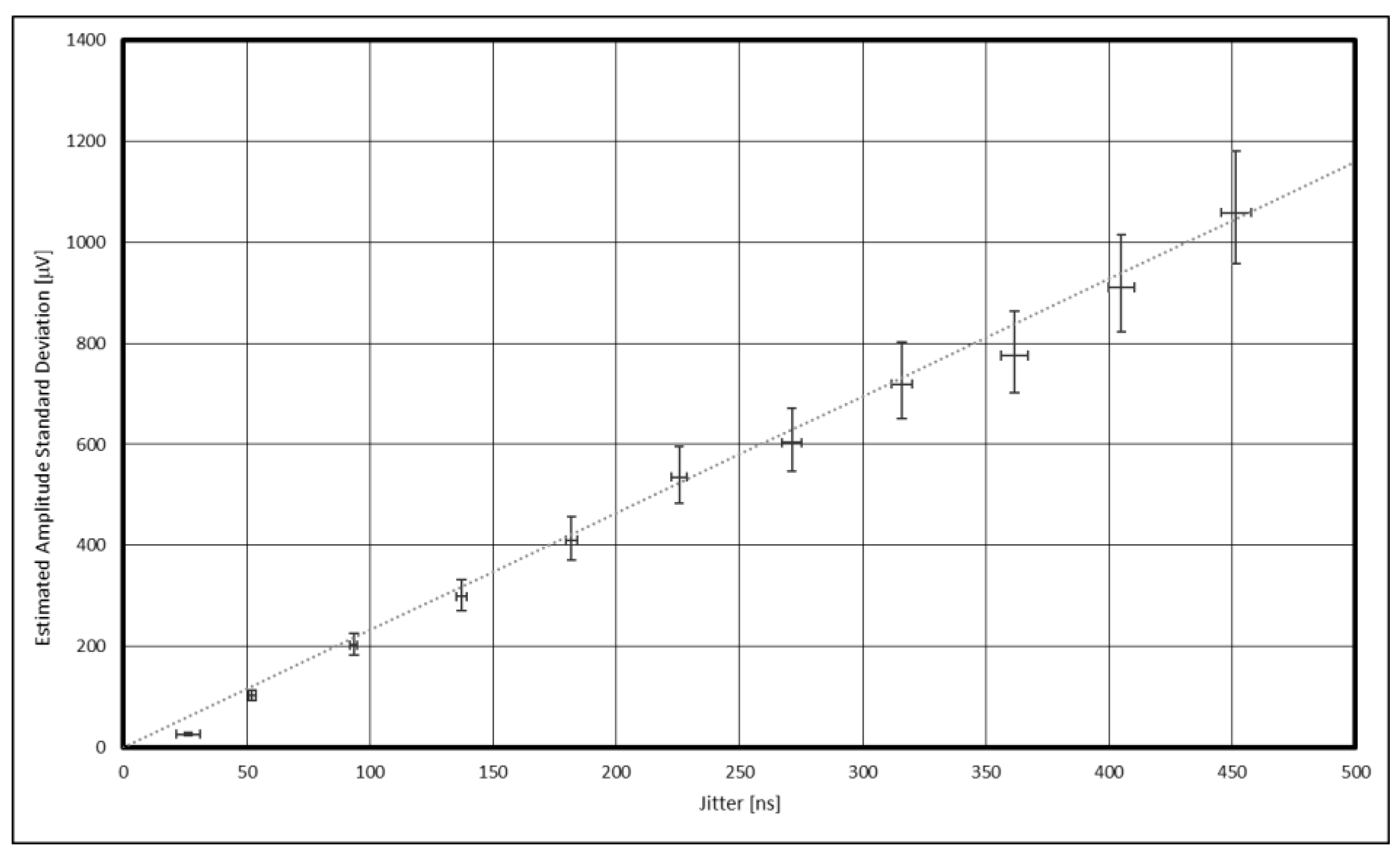
We are thus now able to represent the estimated amplitude standard deviation as a function of jitter. This can be seen in Figure 17. The vertical and horizontal error bars represent the confidence intervals for the estimated sinusoidal amplitude and jitter as shown in the previous two figures. One can observe a linear relationship between the two variables as expected from eq. (28).
A straight line was fitted, in a least squares sense, to the data points and the following relation was obtained:
Comparing this with the expected relation given in (28) we obtain
with
This straight line is depicted in Figure 17 using the dotted trace. A discrepancy was this found between the slopes of the analytical and experimental relationships. This discrepancy is given be the coefficient which was expected to be .
8. Conclusions
In this work a simple analytical expression was derived for the standard deviation of the estimate of the amplitude of a sinewave made using the least squares procedure in the presence of jitter or phase noise. The derivation used a first order Taylor series approximation which was validated using both numerical simulations and experimental data through a Monte Carlo type procedure. The resulting expression can be used not only to compute the confidence interval for sinusoidal amplitude estimation, but also to help choose the number of signal samples to acquire in order to achieve a given bound in estimation precision.
The hardware used in the experimental setup was described in detail. It consisted of two function generators and a data acquisition module. The software developed using National Instruments LabVIEW graphical programming language was presented mentioned but without much detail due to its complexity. The amount of jitter/phase noise present was controlled by phase modulating the clock signal responsible for timing the sample acquisition by the data acquisition module. The type of injected jitter/phase noise was a null-mean normal distributed random one with a controllable standard deviation.
A Monte Carlo method is used to determine the standard deviation of the estimated amplitude, repeated for different levels of injected jitter/phase noise. The results obtained confirm a linear relationship between estimated sinusoidal amplitude and jitter standard deviation. There was, nonetheless a 16% discrepancy between the slope of that relationship whose cause remains unknown. Note that several non-ideal phenomena are present in the experimental setup, namely, additive voltage noise, quantization error, intrinsic jitter in the sampling module, phase noise in the stimulus signal and clock generators and limited noise bandwidth both in the function generator as well as in the data acquisition module. All these factors, however, are believed to be independent of the amount of injected jitter/phase noise and would thus contribute a constant offset to the experimental results and not an error proportional to the amount of injected jitter/phase noise standard deviation as observed. Furthermore, they are present both in the sinewave amplitude estimation and in the jitter/phase noise estimation procedures. The non-accounted for non-ideal phenomena at play must be proportional to the amount of jitter/phase noise produced. Recall that for the numerically simulated tests performed there was no discrepancy found which gave us confidence in the analytical derivations and in the software developed. We thus conclude that it must be due to a hardware phenomenon not accounted for in this work.
In the future one might continue the work presented here by considering, for example, the uncertainty in both amplitude and initial phase in the presence of jitter or phase noise when using the 4-parameter sine fitting algorithm where the signal frequency on not known and must be estimated using an iterative procedure. Other endeavors one might pursue, making use of this work, is the uncertainty of the estimation of other signal parameters like signal-to-noise ratio (SNR) or signal-to-noise and distortion (SINAD) or even the uncertainty of parameters associated with devices or circuits that are inferred from sine fitting of data points like, for example, total harmonic distortion (THD) or amplifier gain.
We hope that this work might be useful to others involved in experimental applications of the sine-fitting procedure and also in the experimental validation of the uncertainty of sine-fitting parameters and their dependence on non-ideal factors.
Author Contributions
All work was carried out by F.A.
Funding
This work is funded by FCT/MCTES through national funds and when applicable co-funded EU funds under the project UIDB/EEA/50008/2020 and FCT/2022.72436.CPCA.A0 whose support the author gratefully acknowledges.
Institutional Review Board Statement
Not applicable.
Informed Consent Statement
Not applicable
Data Availability Statement
The data presented in this study are available on request from the author.
Conflicts of Interest
The author declares no conflicts of interest.
References
- Rao, S. S., Mechanical Vibrations, 4th edition, Prentice Hall (2004).
- Kramer, S. L., Geotechnical Earthquake Engineering, Prentice Hall (1996).
- Dally, J. W., Riley, W. F., & McConnell, K. G., Instrumentation for Engineering Measurements (2nd edition), John Wiley & Sons (1993).
- Queirós, R., Corrêa Alegria, F., Girão, P., Cruz Serra, A., A Multi-Frequency Method for Ultrasonic Ranging, Ultrasonics, Elsevier, vol. 63, pp. 86 93, December 2015. [CrossRef]
- Kay, S. M.: Fundamentals of Statistical Signal Processing, Volume I: Estimation, 1st edition. Pearson (1993), ISBN; 978-0133457117.
- Balestrieri, E.; Picariello, F.; Rapuano, S.; Tudosa, I. Review on jitter terminology and definitions. Measurement 2019, 145, 264–273. [Google Scholar] [CrossRef]
- Reinhardt, V.S.: A Review of Time Jitter and Digital Systems. In: Proceedings of the 2005 IEEE International Frequency and Control Symposium and Exposition, pp. 38–45, Vancouver, Canada (2005).
- Corrêa Alegria, F., Contribution of Jitter to the Error of Amplitude Estimation of a Sinusoidal Signal, Metrology and Measurement Systems, Vol. XVI, nº. 3/2009, M-0317, pp. 465 478, October 2009. 20 October.
- Corrêa Alegria, F., Uncertainty of the Initial Phase Estimation of a Sinewave in the Presence of Phase Noise, Additive Noise or Jitter, Journal of the Franklin Institute, vol. 361, no. 15, October 2024. [CrossRef]
- Corrêa Alegria, F., Xie, L., Pasadas, D., Study of the Bias of the Initial Phase Estimation of a Sinewave of Known Frequency in the Presence of Phase Noise”, MDPI Sensors, vol. 24, no. 3830, June 2024. [CrossRef]
- Corrêa Alegria, F., Bias of Amplitude Estimation Using Three-Parameter Sine Fitting in the Presence of Additive Noise, Measurement, Elsevier Science, vol. 42, no. 5, pp. 748-756, June 2009. [CrossRef]
- Corrêa Alegria, F. and Cruz Serra, A., Gaussian Jitter Induced Bias of Sine Wave Amplitude Estimation Using Three-Parameter Sine Fitting, IEEE Transactions on Instrumentation and Measurement, vol. 59, no. 9, pp. 2328-2333, September 2010. [CrossRef]
- Papoulis, A., Probability, Random Variables and Stochastic Processes, 3rd ed., McGraw-Hill, 1991, p. 156.
- IEEE Standard 802.3-2018 - IEEE Standard for Ethernet.
- PCI-SIG. PCI Express Base Specification Revision 3.0.
- Pohlmann, Ken C., Principles of Digital Audio. McGraw-Hill, 2005.
- Razavi, Behzad, Principles of Data Conversion System Design. Wiley-IEEE Press, 1995.
- Altera Corporation, Timing Closure Methodology for FPGAs, Application Note 191, 2011.
- Misra, Pratap, and Per Enge, Global Positioning System: Signals, Measurements, and Performance. Ganga-Jamuna Press, 2006.
- HDMI Forum, HDMI 2.0 Specification, 2013.
- 3GPP TS 38.104, NR; Base Station (BS) Radio Transmission and Reception, 2018.
- Rohde, Ulrich L., Ajay K. Poddar, and Georg Böck. The Design of Modern Microwave Oscillators for Wireless Applications: Theory and Optimization. Wiley, 2005.
- IEEE Standard for Digitizing Waveform Recorders, in IEEE Std 1057-2017 (Revision of IEEE Std 1057-2007), 26 Jan. 2018. [CrossRef]
Figure 1.
Simulated data points (100 points) for a sinewave with an amplitude of 3 V, an initial phase of π/3 rad and a frequency of 1 Hz, corrupted with phase noise, normally distributed, with null means and a standard deviation of 0.1 rad.
Figure 1.
Simulated data points (100 points) for a sinewave with an amplitude of 3 V, an initial phase of π/3 rad and a frequency of 1 Hz, corrupted with phase noise, normally distributed, with null means and a standard deviation of 0.1 rad.
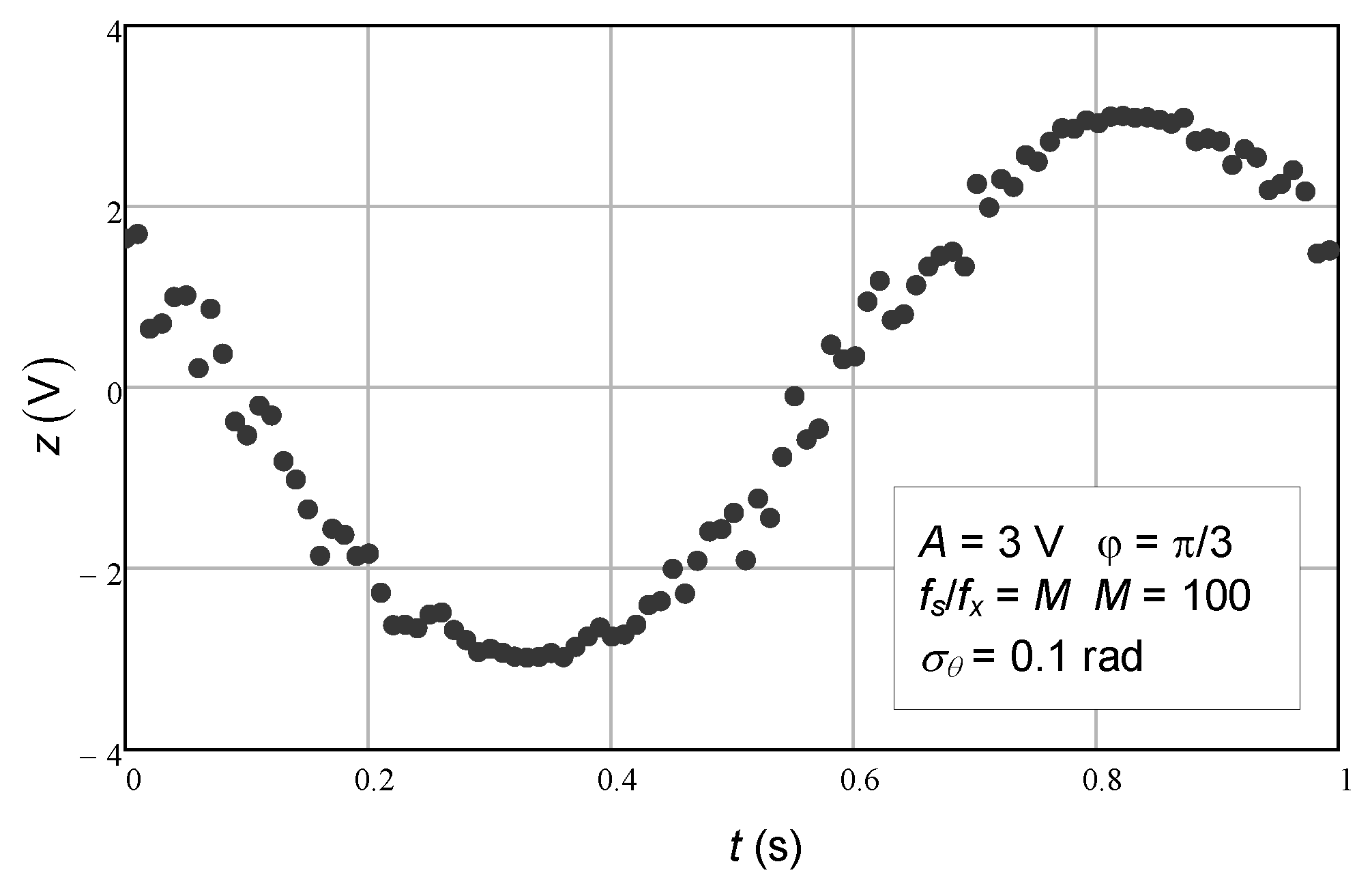
Figure 2.
Standard deviation of the estimated sine wave amplitude as a function of phase noise standard deviation. The circles represent the values obtained with the Monte Carlo analysis. The confidence intervals for a confidence level of 99.9% are represented by the vertical bars. The solid line represents the value given by the theoretical expression (27). The number of repetitions made (R) was 2000.

Figure 3.
Standard deviation of the estimated sine wave amplitude as a function of phase noise standard deviation. The circles represent the values obtained with the Monte Carlo analysis. The confidence intervals for a confidence level of 99.9% are represented by the vertical bars. The solid line represents the value given by the approximate expression (28).

Figure 4.
Standard deviation of the estimated sine wave amplitude as a function of phase noise standard deviation. The circles represent the values obtained with the Monte Carlo analysis for a number of samples of 9. The confidence intervals for a confidence level of 99.9% are represented by the vertical bars. The solid line represents the value given by the approximate expression (27).
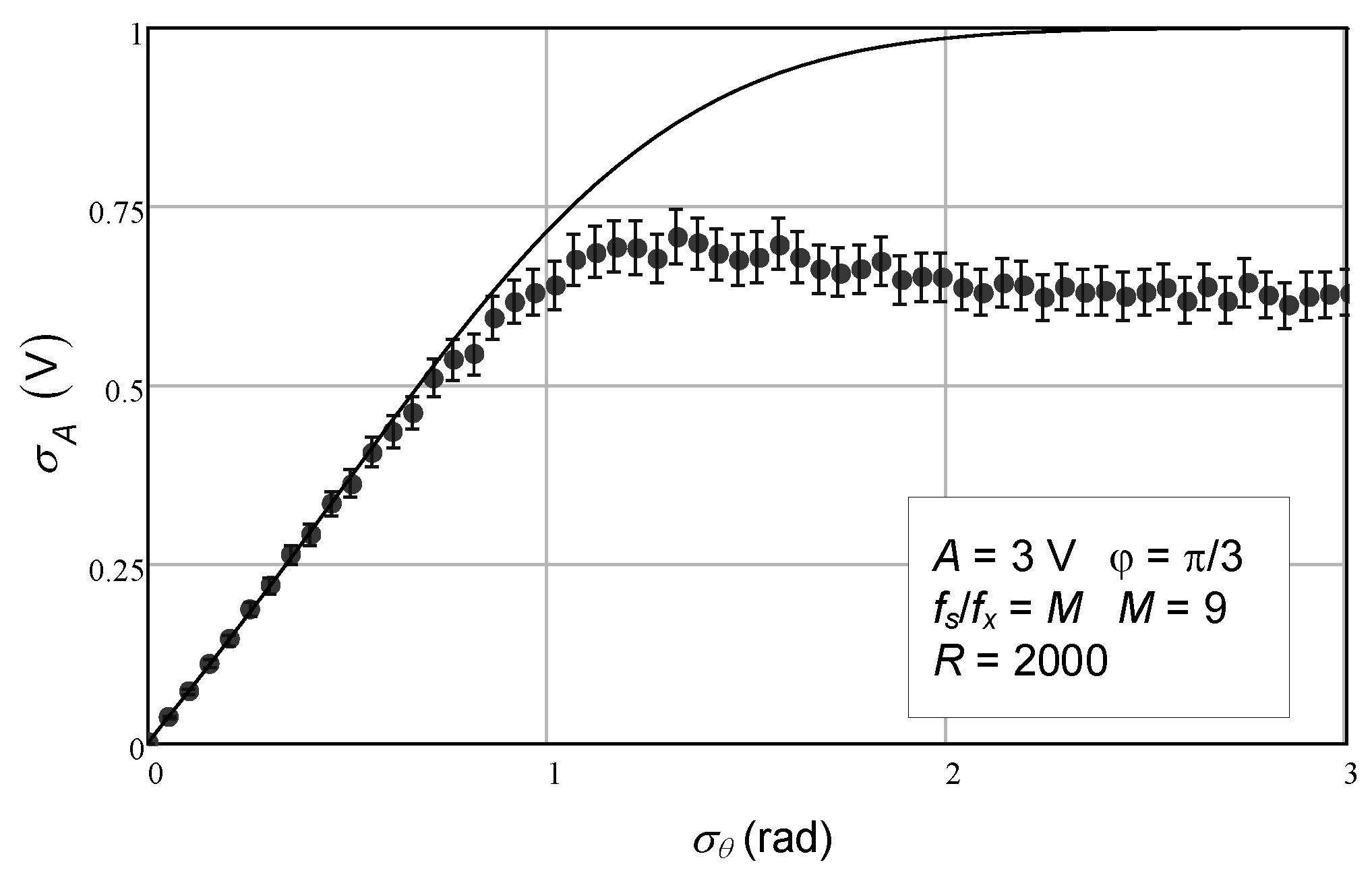
Figure 5.
Standard deviation of the estimated sine wave amplitude as a function of phase noise standard deviation. The circles represent the values obtained with the Monte Carlo analysis for a number of samples of 100. The confidence intervals for a confidence level of 99.9% are represented by the vertical bars. The solid line represents the value given by the approximate expression (27).
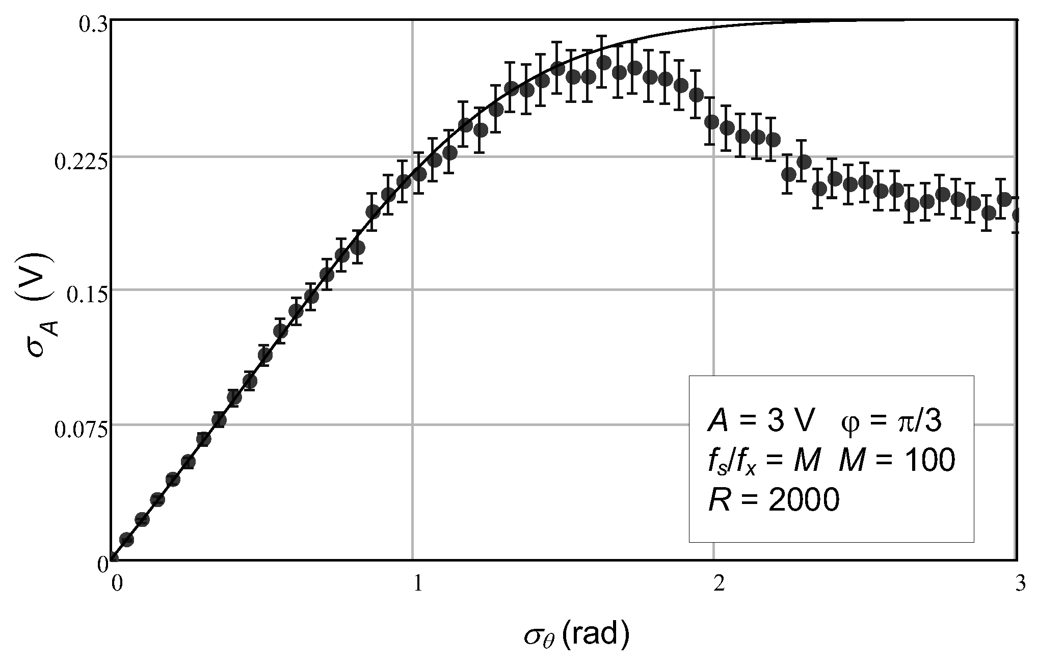
Figure 6.
Standard deviation of the estimated sine wave amplitude as a function of the number of samples. The circles represent the values obtained with the Monte Carlo analysis. The confidence intervals for a confidence level of 99.9% are represented by the vertical bars. The solid line represents the value given by the approximate expression (27).
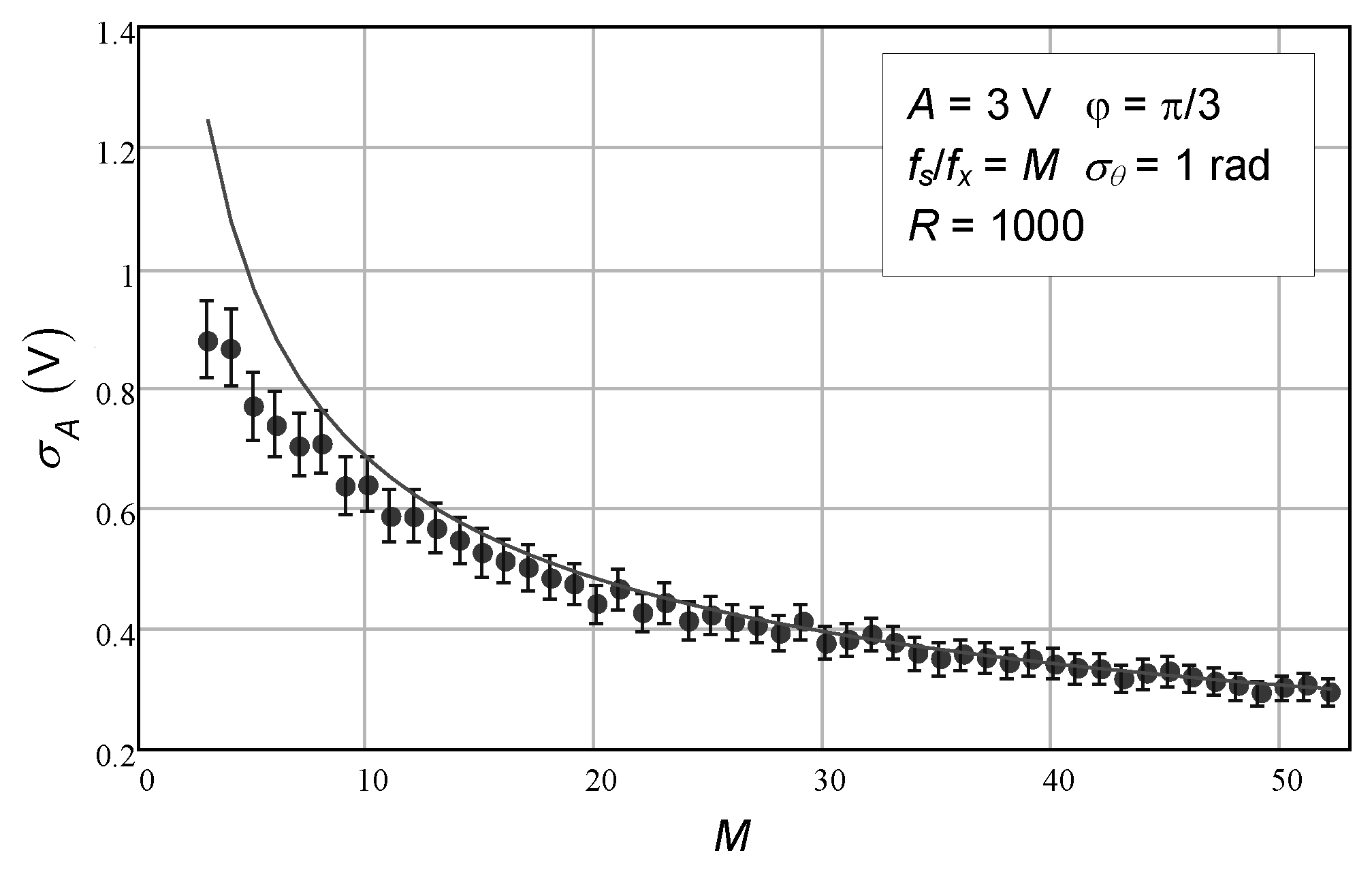
Figure 7.
Hardware setup used to experimentally validate the relationship between jitter and estimated sinewave amplitude. Two function generators were used together with a 16-bit data acquisition module from National Instruments, model NI-USB-6218 (seen on top) connected through a USB interface with a personal computer (seen partially on the right). One of the function generators, model DS360 from Stanford Research (bottom) was used to create the sinusoidal stimulus signal. The other function generator, model AG3320A from Agilent (middle), was used to create the clock signal that controlled the sampling instants, and which was modulated by internally generated, normally distributes, phase noise.
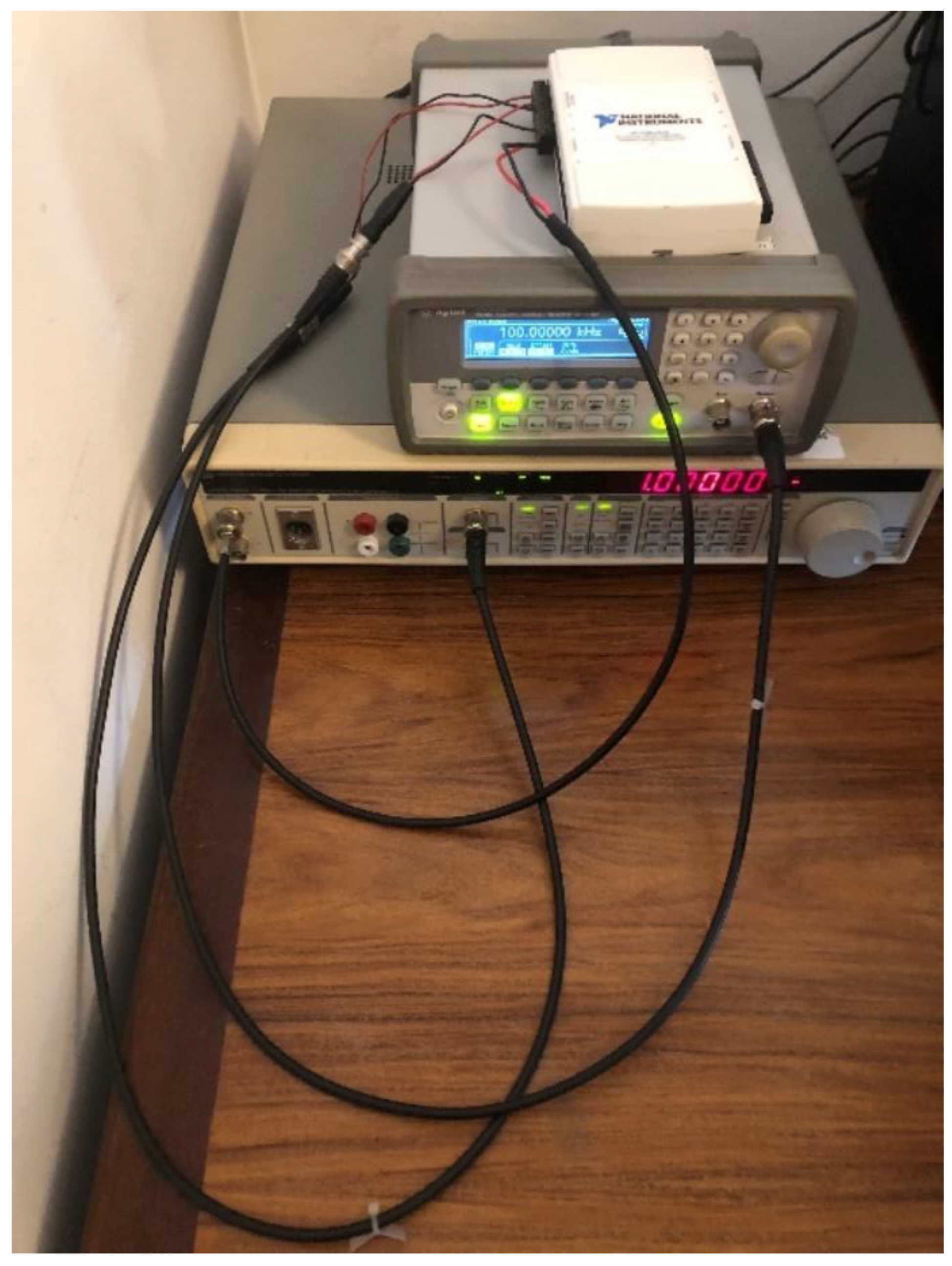
Figure 8.
Pinout of the data acquisition module from National Instruments, model NI-USB-6218.
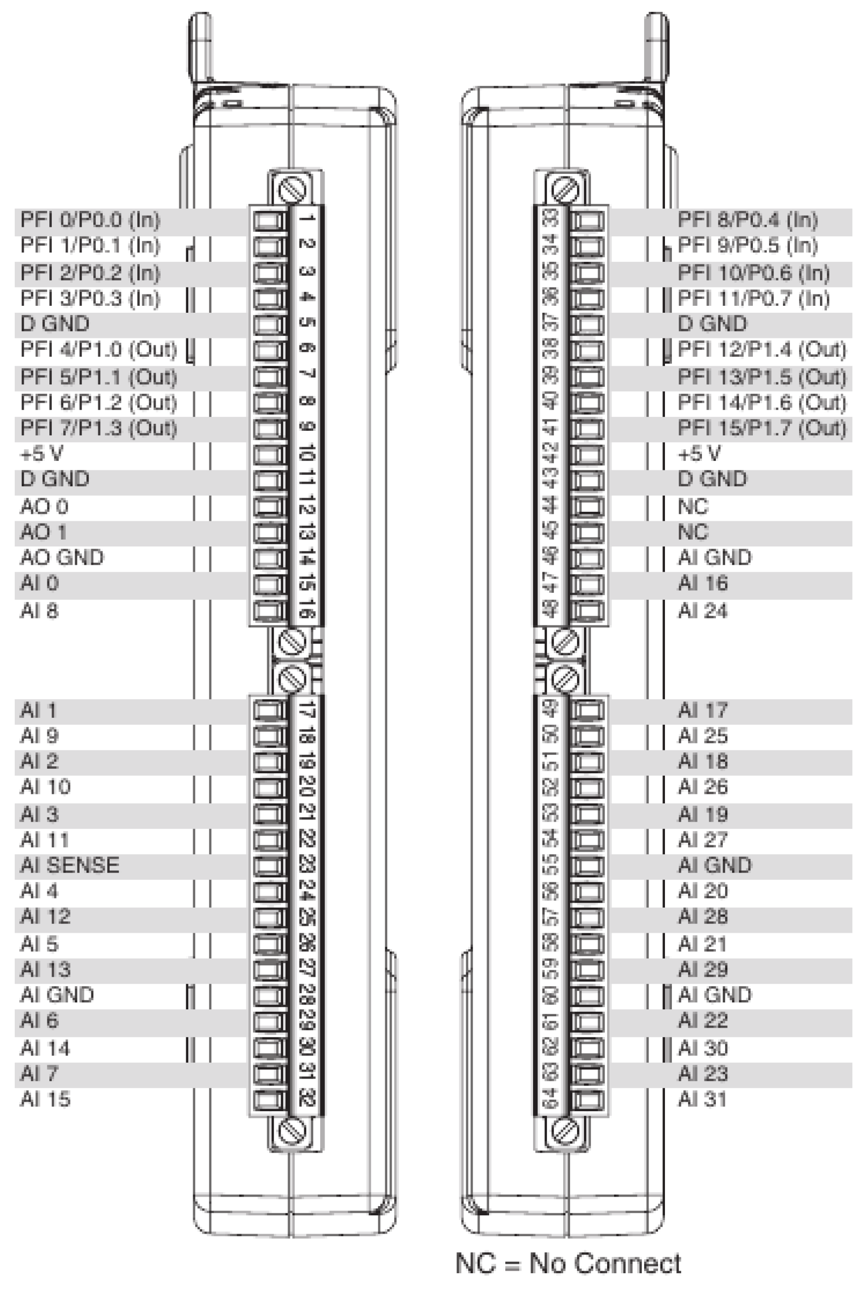
Figure 9.
Block diagram of the test setup where one can observe the personal computer, the data acquisition module and the two general purpose function generators.
Figure 9.
Block diagram of the test setup where one can observe the personal computer, the data acquisition module and the two general purpose function generators.
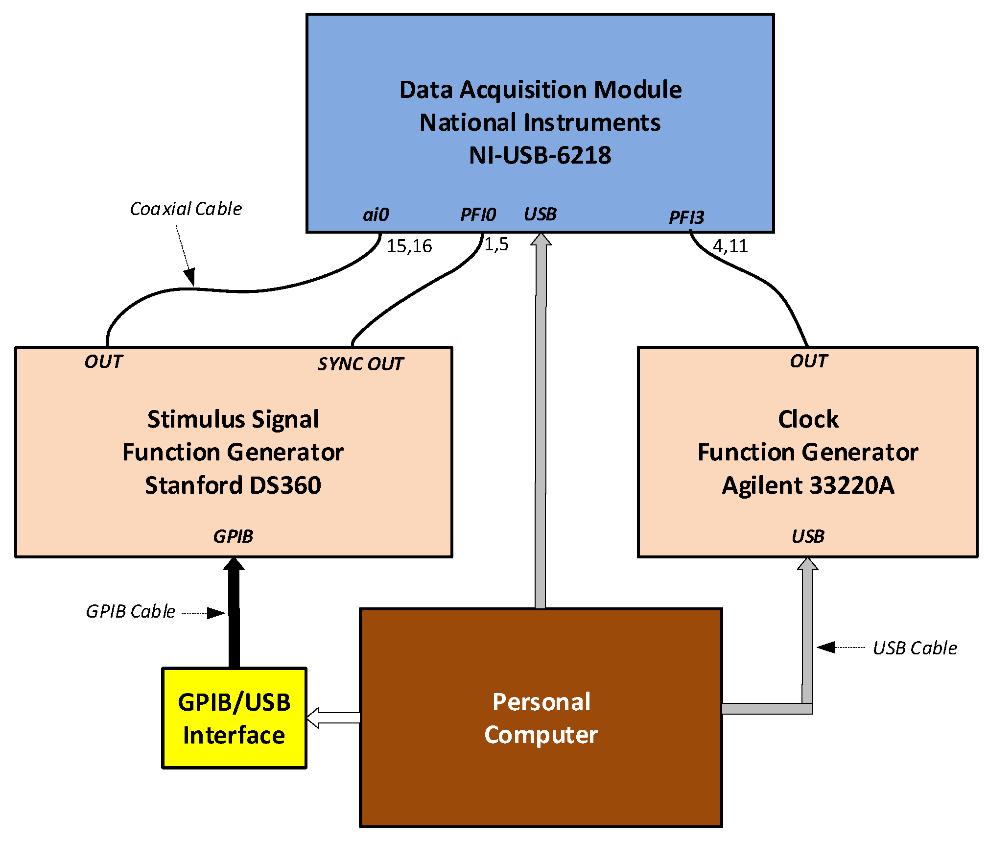
Figure 10.
Photograph of the USB/GPIB Interface module from Keysight, model 82357B connected to the Stanford Research DS360 generator to the right. The cable to the left of the image has an USB interface and goes to the personal computer.
Figure 10.
Photograph of the USB/GPIB Interface module from Keysight, model 82357B connected to the Stanford Research DS360 generator to the right. The cable to the left of the image has an USB interface and goes to the personal computer.
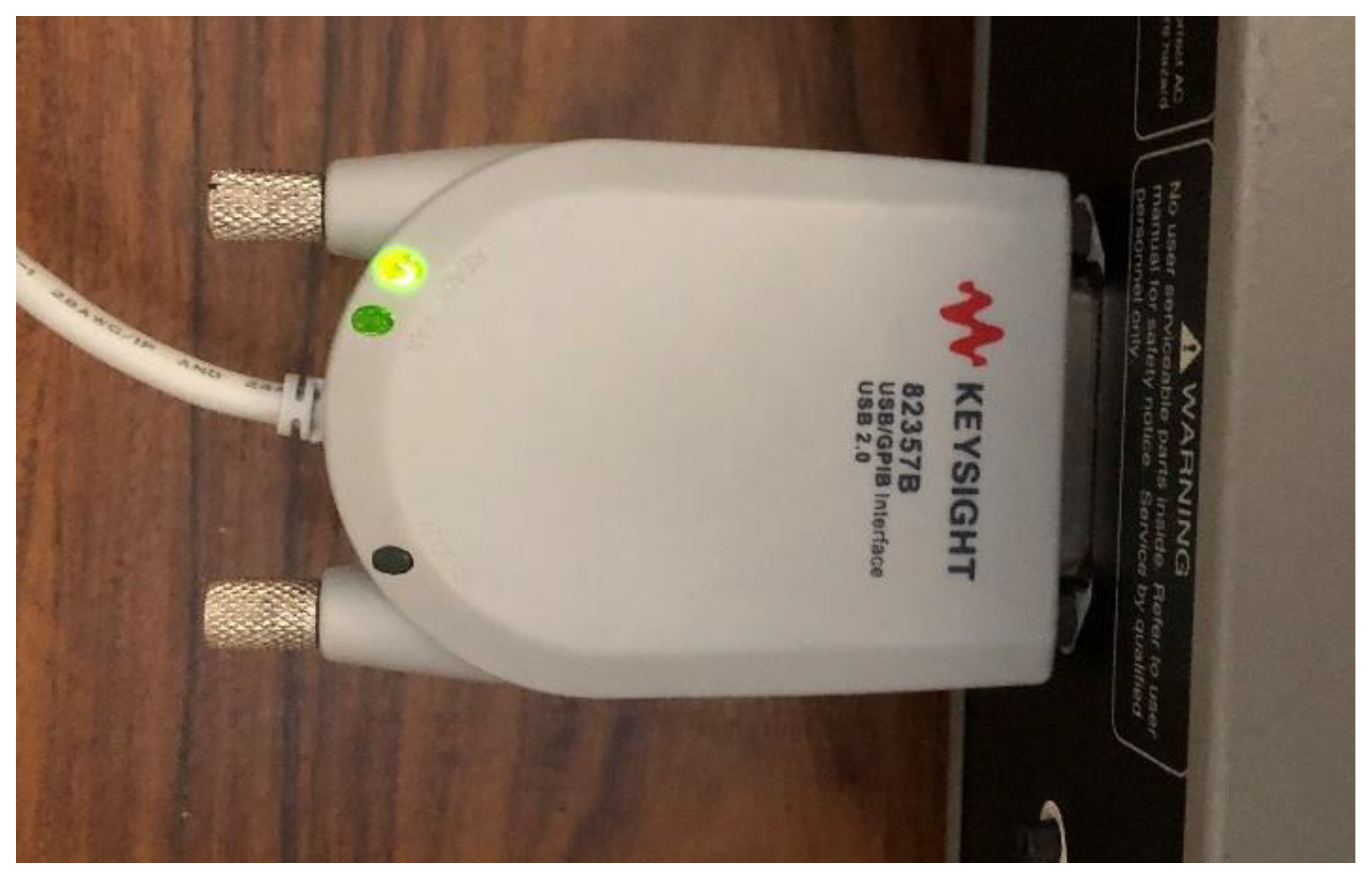
Figure 11.
Partial image of one of the front panels of the LabVIEW application developed. Some parts shown are not relevant to the present work. On the left side we observe the data acquisition module settings like range, sampling frequency, number of samples and terminals used. In the middle we the ADC parameters like the number of bits and the type of transfer function of the ADC. On the right-side e see the function generators used with their addresses as well as their configuration like amplitude, frequency and waveform shape.
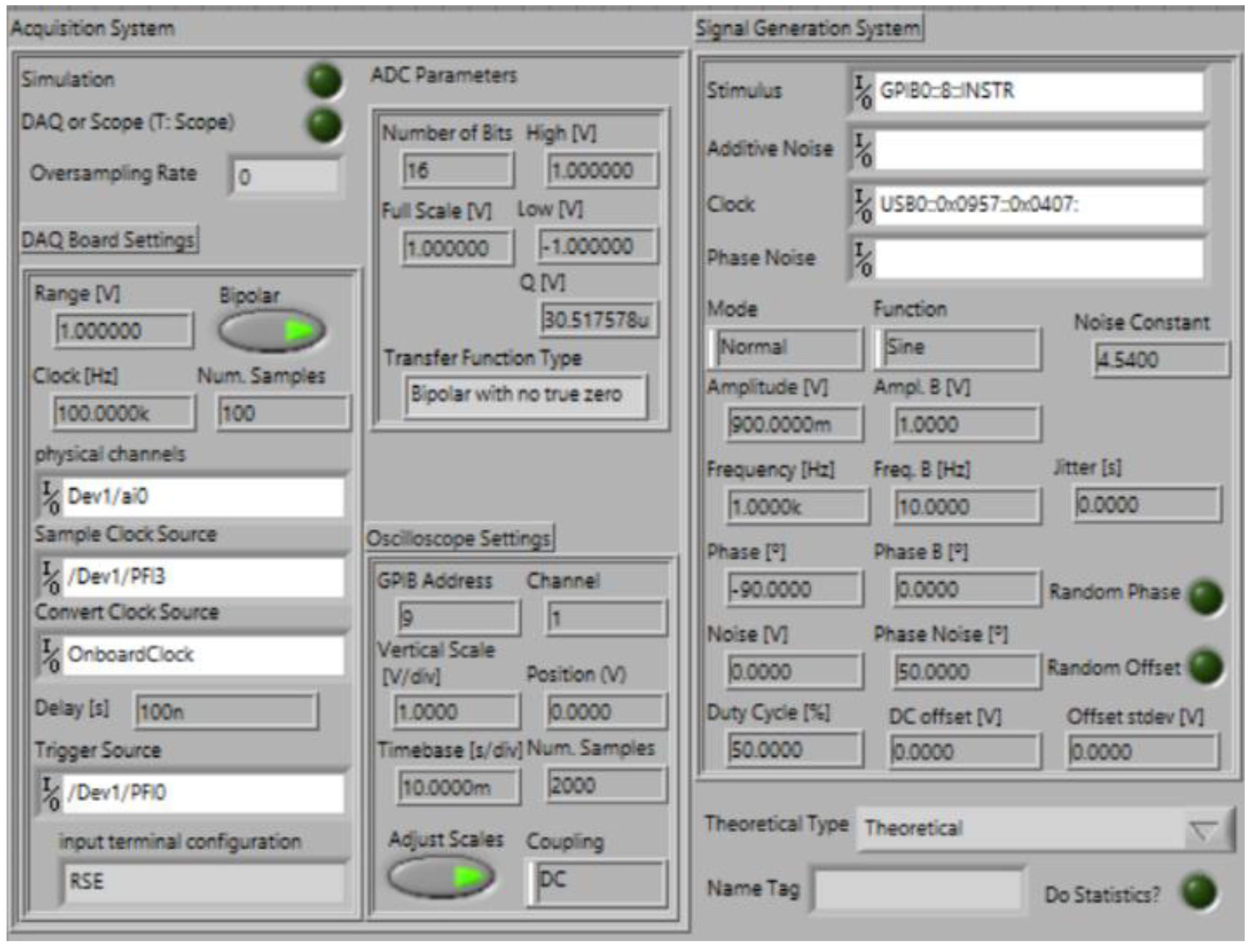
Figure 12.
Image of the block diagram of the virtual instrument that carries out the sinewave test. It starts by computing the setup parameters to used (left part) in the subVI “Prepare Sinewave Test” which are then used to program the function generators in the “Control FGs” subVI. The data acquisition samples are then acquired in the “Acquire or Simulate” subVI and finally the data points gathered are used to estimate different parameters like sinewave amplitude and initial phase.
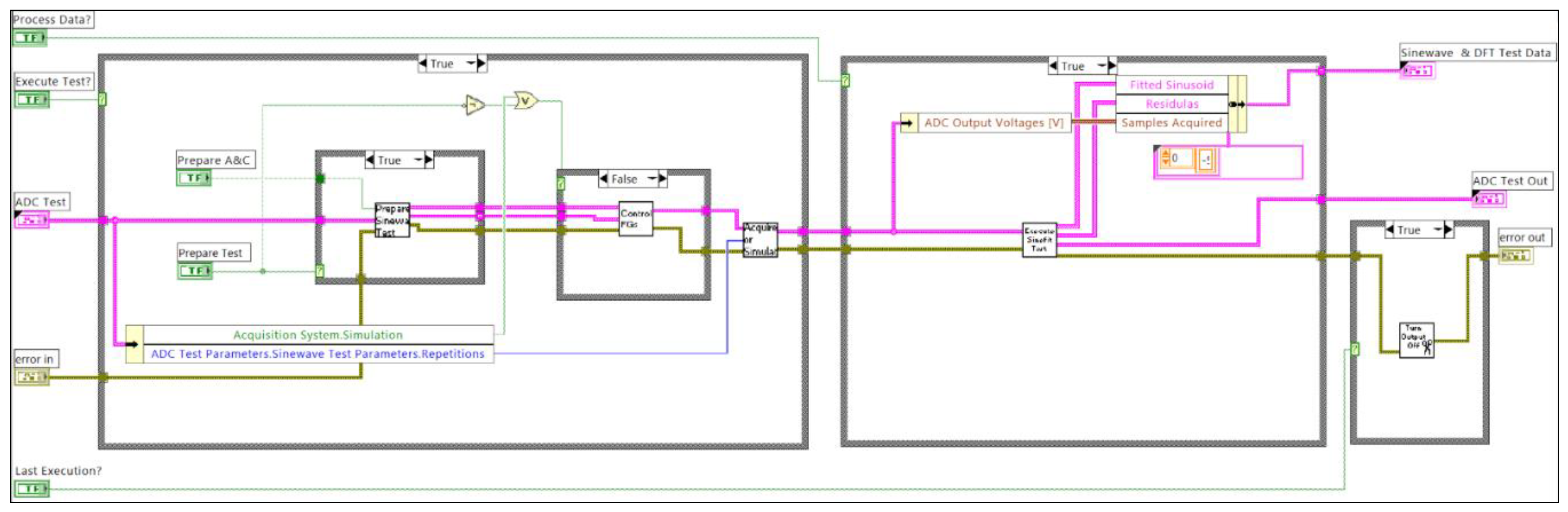
Figure 13.
Image of the front panel portion that shows the result of amplitude estimation as a function of the clock generator phase noise. Each data point is represented by a circle and an error bar. The theoretical expected values are shown with a solid line.
Figure 13.
Image of the front panel portion that shows the result of amplitude estimation as a function of the clock generator phase noise. Each data point is represented by a circle and an error bar. The theoretical expected values are shown with a solid line.
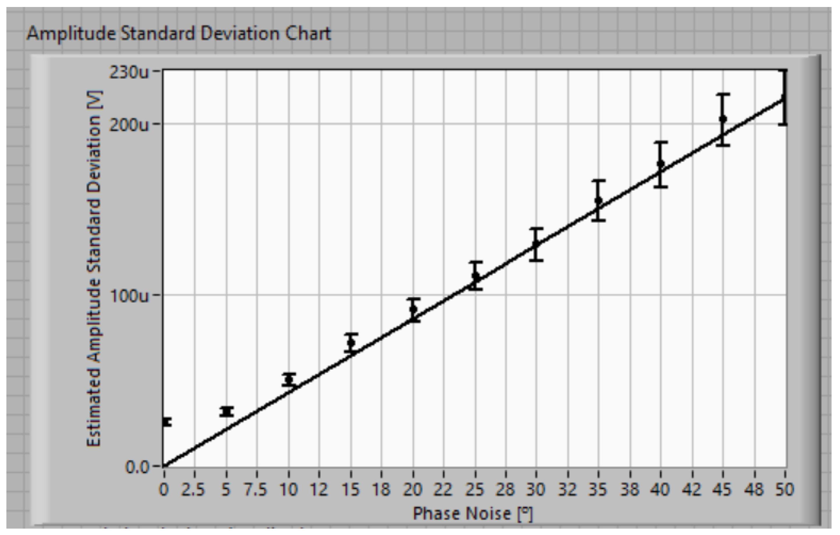
Figure 14.
Image of the block diagram responsible for repeating the test a certain number of times in order to compute the mean and standard deviation of the estimated values of sinewave amplitude, initial phase and offset.
Figure 14.
Image of the block diagram responsible for repeating the test a certain number of times in order to compute the mean and standard deviation of the estimated values of sinewave amplitude, initial phase and offset.
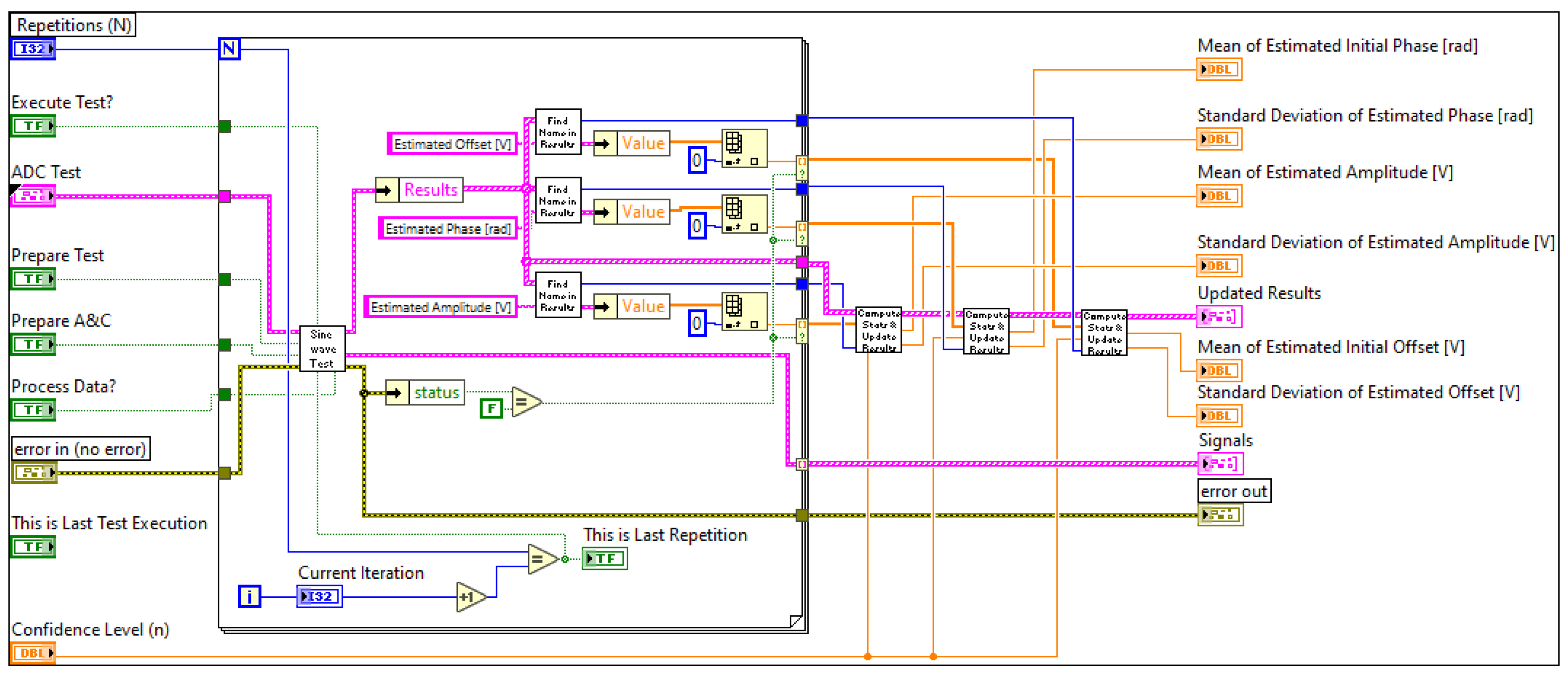
Figure 15.
Image of the block diagram responsible estimating the sinewave amplitude, initial phase and DC value given the data points and the sinewave frequency.
Figure 15.
Image of the block diagram responsible estimating the sinewave amplitude, initial phase and DC value given the data points and the sinewave frequency.
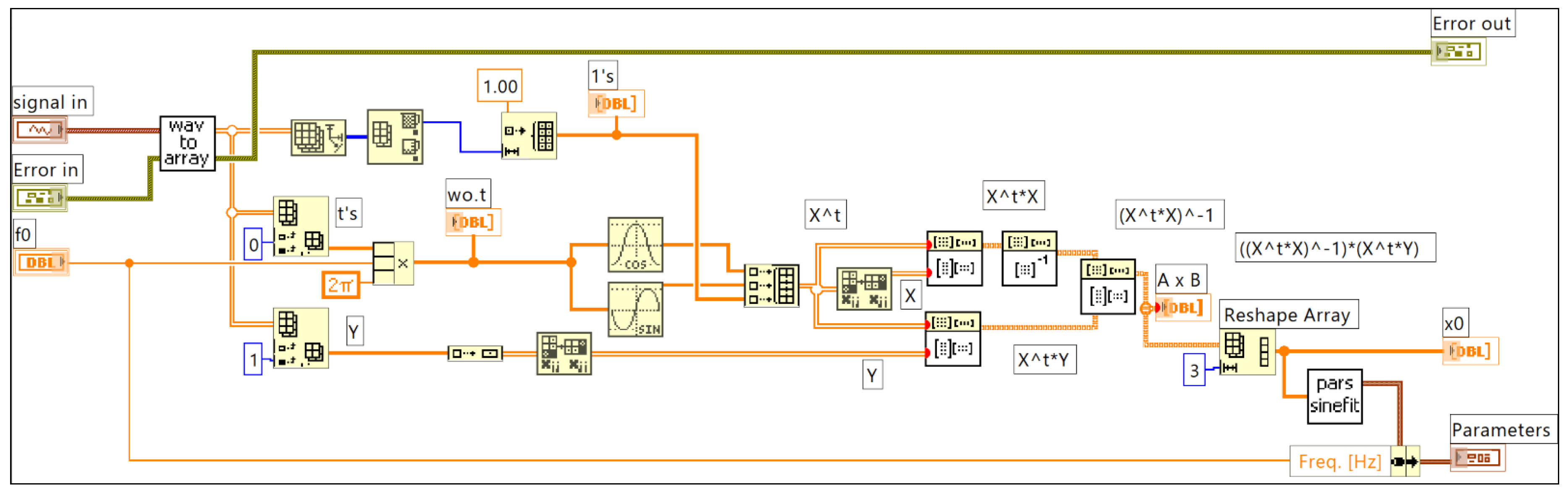
Figure 15.
Chart containing the experimentally estimated sinewave standard deviation as a function of the injected amount of phase noise.
Figure 15.
Chart containing the experimentally estimated sinewave standard deviation as a function of the injected amount of phase noise.
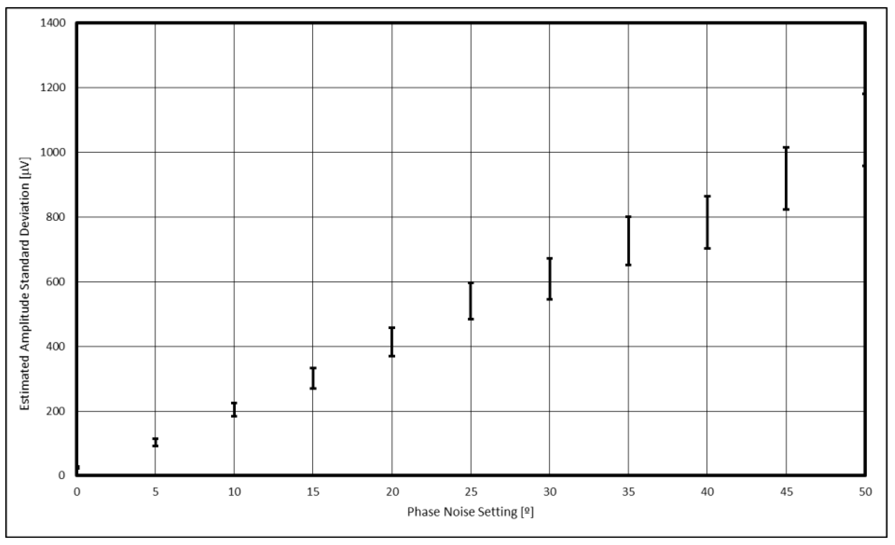
Figure 16.
Representation of the relation between the measured values of phase noise standard deviation and the configured values of phase noise standard deviation.
Figure 16.
Representation of the relation between the measured values of phase noise standard deviation and the configured values of phase noise standard deviation.
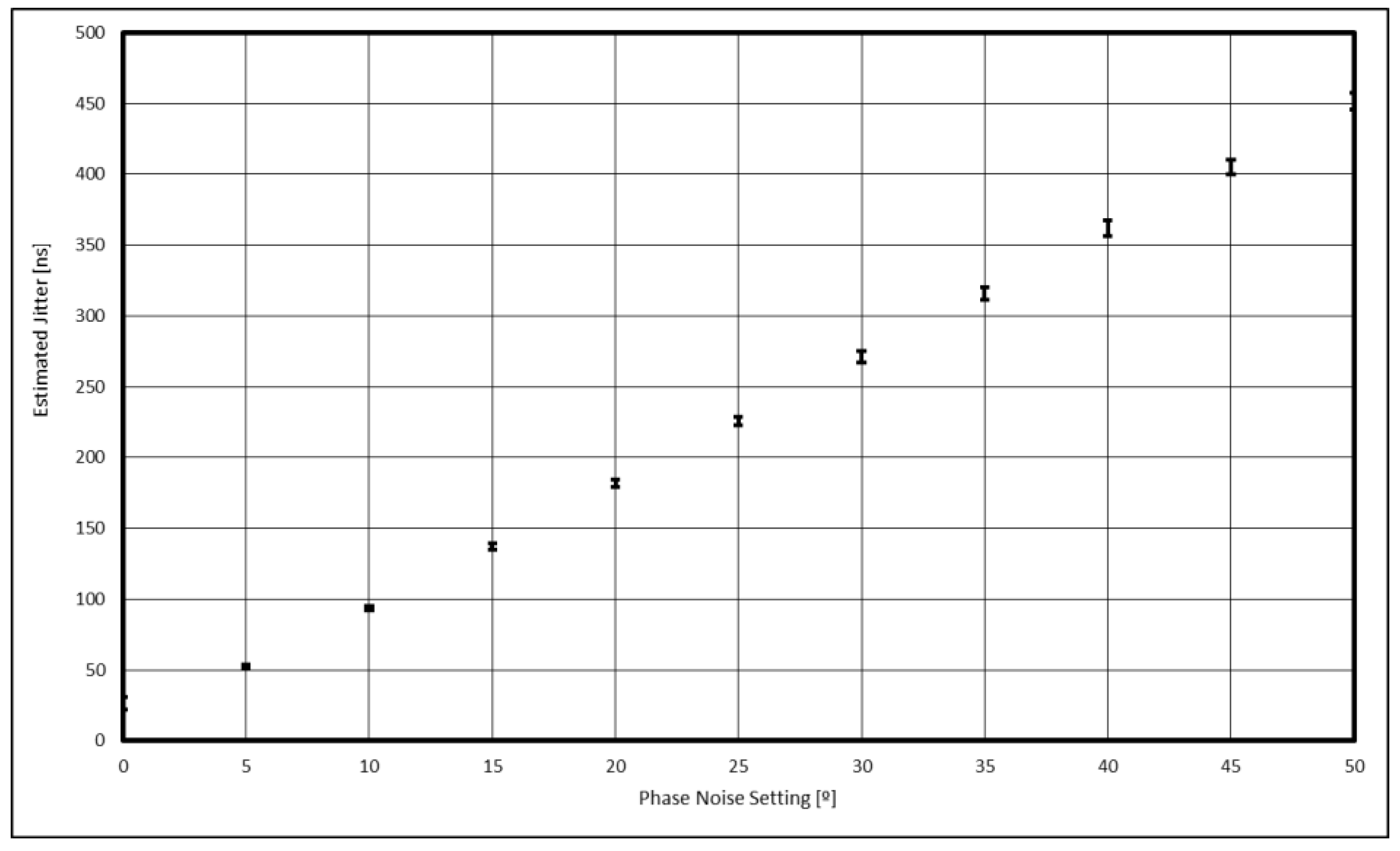
Figure 17.
Experimental estimated amplitude standard deviation as a function of sampling jitter present. The error bars represent the confidence intervals for the estimation of both the amplitude estimation carried out with the least-squares sine-fitting method and the estimated amount of jitter present. The dashed line represents the straight line that best fits the data points.
Disclaimer/Publisher’s Note: The statements, opinions and data contained in all publications are solely those of the individual author(s) and contributor(s) and not of MDPI and/or the editor(s). MDPI and/or the editor(s) disclaim responsibility for any injury to people or property resulting from any ideas, methods, instructions or products referred to in the content. |
© 2024 by the authors. Licensee MDPI, Basel, Switzerland. This article is an open access article distributed under the terms and conditions of the Creative Commons Attribution (CC BY) license (http://creativecommons.org/licenses/by/4.0/).
Copyright: This open access article is published under a Creative Commons CC BY 4.0 license, which permit the free download, distribution, and reuse, provided that the author and preprint are cited in any reuse.


