Submitted:
19 November 2024
Posted:
19 November 2024
You are already at the latest version
Abstract
As the logistics industry modernizes, living standards improve, and consumption patterns shift, the demand for fresh food continues to grow, making cold chain logistics for perishable goods a critical component in ensuring food quality and safety. However, the presence of both soft and hard time windows among demand nodes can complicate single-network distribution of perishable goods. In response to these challenges, this paper proposes an optimization model for multi-distribution center perishable goods delivery, considering both one-echelon and two-echelon network joint distribution. The model aims to minimize total costs, including transportation, fixed, refrigeration, goods damage, and penalty costs, all while measuring customer satisfaction by the start time of service at each demand node. A two-stage heuristic algorithm is designed to solve the model. In the first stage, an initial solution is constructed using a greedy approach, based on the principles of the k-medoids clustering algorithm that considers both spatial and temporal distances. In the second stage, the initial routing solution is optimized using a linear programming approach from the Ortools solver combined with an Improved Adaptive Large Neighborhood Search (IALNS) algorithm. The effectiveness of the proposed model and algorithm is validated through a case study analysis. Results indicate that the enhanced algorithm achieves faster convergence and more effective overall cost optimization.
Keywords:
Joint distribution in one-echelon and two-echelon networks
; soft and hard time windows
; Perishable Goods Distribution
1. Introduction
As living standards improve, the demand for perishable goods has progressively increased, making cold chain logistics a crucial component for ensuring these products reach consumers fresh and safe [1]. Beyond meeting customer expectations for product quality, service quality also plays a significant role in influencing customer satisfaction, which can be measured by the timeliness of product delivery. Consequently, delivering products within the time frames specified by customers is becoming increasingly important [2]. In real-world distribution, customers often specify desired delivery time intervals, requiring that delivery vehicles arrive within these periods. Depending on the strictness of the delivery time requirements, time windows are classified as either soft time windows or hard time windows [3]. Current research on cold chain distribution pathways for perishable goods typically considers either one-echelon or two-echelon networks alone. However, given that demand nodes frequently present varying and concurrent soft and hard time window requirements, single-network distribution in either one-echelon or two-echelon networks alone cannot adequately meet these time window demands at demand nodes. To address this issue more effectively, an optimization model for joint distribution of perishable goods across one-echelon and two-echelon networks is established. With the aim of minimizing total costs, the model is employed to determine the distribution routes of vehicles, considering the satisfaction levels at demand nodes.
The remainder of this paper is organized as follows: Section 2 provides a review of literature related to this paper. In Section 3, an optimization model for joint distribution of perishable goods across one-echelon and two-echelon networks is developed, addressing time satisfaction at both rigid and flexible demand nodes, a two-stage heuristic algorithm is introduced in Section 4. Section 5 details a case study that validates the effectiveness of the model and algorithm. Comparisons between the solutions from the first and second stages demonstrate that the initial solution obtained through the first stage is optimal, and the second stage shows improved optimization performance. Conclusions and potential future research avenues are discussed in Section 6.
2. Literature Review
Dantzig and Ramser were the pioneers in formulating the Vehicle Routing Problem (VRP) and developed its first heuristic algorithm [4]. As application scenarios evolved, research on VRP has expanded significantly. The Vehicle Routing Problem for Perishable Goods (VRPPG) is a subset of VRP, dealing specifically with products that rapidly deteriorate in quality [5]. The distribution of perishable goods was first addressed by Tarantilis and Kiranoudis who studied the Hybrid Fleet Vehicle Routing Problem (HFFVRP) and solved it using a metaheuristic threshold acceptance algorithm [6]. In the field of one-echelon network distribution paths for perishable goods, with the goal of minimizing unit costs while maximizing customer satisfaction, Gao Yuan Qin et al. assessed delivery punctuality as a measure of customer satisfaction. They developed a cold chain vehicle routing model and designed a genetic algorithm for its solution. Additionally, the impact of increased carbon pricing on emissions, customer satisfaction, and total costs was examined [7]. Anil Kumar Agrawal et al. addressed the vehicle routing problem for perishable goods using heterogeneous fleets. They incorporated time windows and quality requirements for perishable goods into the distribution process, established a mixed nonlinear programming model, and applied a genetic algorithm for its resolution [8]. With objectives of minimizing transportation costs, spoilage costs, and carbon emissions, and maximizing customer satisfaction, Zulvia et al. considered varying transportation times during peak and off-peak periods. They constructed a multi-objective perishable goods vehicle routing model and implemented a multi-objective gradient evolution algorithm for its solution [9]. Jiang Li et al. aimed to minimize the total cost and maximize customer satisfaction, taking into account customer appointment time windows. They crafted a multi-objective fresh produce delivery path model and employed an elitist strategy-based non-dominated sorting genetic algorithm for its resolution [10]. Focusing on minimizing total costs, with specific goals of minimizing quality loss costs and transportation costs, Partha Sarathi Barma and associates considered the distribution to two types of customers using refrigerated and standard vehicles. They established a multi-objective m-ring star-shaped distribution network model and utilized a non-dominated sorting genetic algorithm and strength Pareto evolutionary algorithm for its solution [11]. Huai and team aimed to minimize distribution costs and goods damage costs in their study. They constructed a multi-type vehicle routing model for perishable goods and solved it using a genetic algorithm based on two decoding methods [12].
The two-echelon VRP for perishable goods is a variant of the VRP that involves coordination between vehicular routes across two distinct hierarchical levels. In the realm of two-echelon networks for the distribution of perishable goods, objectives such as minimizing costs, reducing carbon emissions, and maximizing customer satisfaction are paramount. Wang Z et al. considered mixed time windows and carbon trading policies, developing a two-echelon cold chain vehicle routing model, and employed an adaptive genetic algorithm for its solution. Their research also examined the impact of variations in mixed time windows, the integration of customer satisfaction, and carbon trading policies on the model [13]. Aiming to minimize transportation and handling costs, reduce customer waiting times, and cut carbon emissions, Sahraeian R et al. considered customer satisfaction and distribution center capacity constraints. They developed a multi-objective mixed integer nonlinear programming model, which was solved using a non-dominated sorting genetic algorithm. The effectiveness of this algorithm was validated through small, medium, and large-scale case studies [14]. In their research, Jaigirdar and colleagues aimed to minimize the total cost, average lead time for the delivery of fresh agricultural products, and initial investment cost for refrigerated distribution centers. They developed a two-echelon multi-objective mixed integer linear programming model for perishable goods. The CPLEX solver was employed to solve this model [15]. Targeting minimal total distribution costs, Ma Yanfang et al. considered the importance of customers, differentiating between regular and key customers. They constructed a two-echelon capacity-constrained vehicle routing optimization model and designed a two-stage heuristic algorithm for solving it. The first stage involved an enhanced genetic simulated annealing algorithm for the two-echelon distribution paths, while the second stage employed an exact method for the one-echelon distribution paths. The effectiveness of these algorithms was demonstrated through case study analysis [16].
Extensive research has been conducted on the vehicle route optimization problem for perishable goods distribution, yielding a wealth of theoretical results. However, most studies focus on one-echelon or two-echelon network distributions independently, predominantly considering single time window requirements, with few addressing both soft and hard time windows. In reality, demand nodes may have differing time requirements for services, potentially necessitating both soft and hard time windows for the delivery of perishable goods. A single network distribution may not suffice to meet these diverse needs. In response to this issue, an optimization model for joint distribution of perishable goods across multiple distribution centers within one-echelon and two-echelon networks is constructed, addressing demand node satisfaction within soft and hard time windows. To enhance solution efficiency, a two-stage heuristic algorithm is designed and its effectiveness is validated through a case study analysis.
3. One-Echelon and Two-Echelon Networks Model
An optimization model has been developed for the joint distribution of perishable goods, addressing satisfaction at two types of demand nodes within one-echelon and two-echelon networks. This model is noted for its complexity and numerous constraints, and is classified as an NP-hard problem. Due to the difficulties in obtaining optimal solutions with exact algorithms, a heuristic approach is employed for the solution. The model aims to minimize total costs and introduces a two-stage heuristic algorithm for this purpose. In the first stage, vehicle routing initial solutions are derived using a combination of k-medoids and greedy algorithms. The k-medoids algorithm, known for its robustness as it is not influenced by outliers and adapts well to various distributions, is utilized to cluster demand nodes. Considering the impact of initial cluster centers on clustering outcomes, the K-Means++ initialization method is employed to enhance the quality and efficiency of clustering. Subsequently, initial routing paths are constructed using a greedy algorithm. In the second stage, an improved Adaptive Large Neighborhood Search (ALNS) algorithm based on linear programming is proposed, leveraging the linear programming capabilities of the Ortools solver. This approach enhances the flexibility and local search capabilities, optimizing the initial paths obtained in the first stage.
3.1. Description of the Problem
A basic discrete undirected road traffic network is considered, where inrepresents the set of nodes. Here, denotes the supply point, the collection of distribution center nodes, and the set of customer nodes is subdivided intowhere;indicates nodes with hard time window requirements, andindicates nodes with soft time window requirements.Letrepresent first-echelon network, with being the nodes accessible for first-echelon vehicle distribution.comprises the edges in the one-echelon network. is defined as second-echelon network, where encompasses nodes accessible for second-echelon vehicle distribution, and constitutes the edge set of the second-echelon network. The supply point has fuel vehicles each with a carrying capacity of and an average speed of . The distribution center node utilizes electric vehicles each with a carrying capacity of , an average speed of , and a maximum travel distance . The number of nodes with soft time window requirements is , while those with hard time window requirements number . Each customer node has a demand . The distance between any two points is . Soft time window nodes expect service within the time window and accept service within , whereas hard time window nodes accept service strictly within . Given the limitations of single-network distribution in satisfying the time window requirements of some hard time window nodes, fuel vehicles in are scheduled to deliver perishable goods directly from the supply point to the nodes . Concurrently, perishable goods are transported from the supply point to the distribution centers, where electric vehicles in continue the delivery to customer nodes , ensuring all demands are met. In scenarios with multiple distribution centers, customer satisfaction regarding time is considered, aiming to minimize total costs (including fixed, refrigeration, transportation, goods spoilage, and time penalty costs). Strategies for joint one-echelon and two-echelon network distribution of perishable goods are developed and analyzed.
The model is based on the following assumptions:
- (1)
- The locations and numbers of supply points, distribution centers, and demand nodes are known.
- (2)
- The demands and service times at demand nodes are predefined and known.
- (3)
- Upon arrival at a distribution center, one-echelon delivery vehicles unload their products, which are immediately loaded onto other one-echelon vehicles, with negligible handling time at the distribution center.
- (4)
- Each demand node is visited only once.
- (5)
- All soft time window demand nodes are serviced through distribution centers.
- (6)
- There are no vehicle paths between distribution centers.
The joint distribution paths for perishable goods in the one-echelon and two-echelon networks are illustrated in Figure 1. In this cold chain network, there is one supply point, three distribution centers, and multiple types of demand nodes, serviced by several one-echelon fuel refrigerated vehicles and a specified number of two-echelon electric refrigerated vehicles. According to the demand at the nodes, perishable goods are either directly delivered to certain hard time window demand nodes by one-echelon vehicles or transported from the supply point to distribution centers, from where two-echelon vehicles distribute them to remaining demand nodes.
3.2. Notation Definition
3.3. Cost Analysis
(1) Fixed Vehicle Costs
Fixed vehicle costs chiefly refer to the expenses associated with operating each vehicle within both one-echelon and two-echelon distribution networks. These costs include driver salaries, vehicle depreciation, and maintenance fees, and are primarily related to the number of refrigerated vehicles utilized.
(2) Variable Transport Costs
The transportation costs of a vehicle refer to the expenses incurred during the vehicle's operation, primarily fuel and electricity consumption. These costs are dependent on the distance traveled and the vehicle’s load capacity.
(3) Refrigeration Costs
To ensure the freshness of perishable goods, refrigerated vehicles are employed for delivery. The refrigeration costs during delivery typically encompass the costs of refrigerants used to maintain the internal temperature of the cargo area. These costs include the energy consumed to keep the temperature low during transport and the additional energy required when the vehicle doors are opened during unloading, which causes an increase in the internal temperature.
(4) Cost of Goods Spoilage
The cost of goods spoilage refers to losses incurred due to the deterioration, rotting, and spoilage of products during transportation and service operations (such as when doors are opened) in cold chain logistics. A decay function is introduced from the literature. It models the quality degradation of perishable products, denoted as . The spoilage rate varies because of the difference in the temperature inside the vehicle during delivery and when the doors are opened for unloading. It is posited that the spoilage rate during transportation is , and changes to when the doors are opened, due to increased air convection and subsequent rise in temperature within the vehicle. The cost of goods spoilage can thus be represented as Equation (4).
(5) Time Penalty Costs
Time window penalty costs include costs associated with early arrival within a hard time window, penalties for late arrival, early arrival penalties within a soft time window, and penalties for late arrival within a soft time window.
(6) Satisfaction Function at Demand Nodes
The satisfaction function for demand nodes is incorporated through a membership function that accounts for service initiation times, assessing the satisfaction levels of demand nodes within a soft time window.
For demand nodes within a hard time window, the satisfaction function is defined as Equation (7).
3.4. Model Development
The model is constructed considering the objectives and all constraints.
Equation (8) is aimed at minimizing the total costs. Equation (9) is designed to enforce satisfaction constraints at demand nodes with soft time windows. Equation (10) is formulated to enforce satisfaction constraints at demand nodes with hard time windows. Equations (11) and (12) are intended to limit the load capacity of one-echelon vehicles. Equations (13) and (14) ensure that each demand node is serviced by only one vehicle. Equation (15) stipulates that each one-echelon vehicle departing from a supply point must return to that supply point. Equation (16) dictates that each two-echelon vehicle departing from a distribution center returns to that distribution center. Equation (17) limits the use of each one-echelon vehicle to a single operation. Equation (18) limits the use of each two-echelon vehicle to a single operation. Equation (19) assigns each demand node to a distribution center. Equation (20) ensures that no vehicular paths exist between distribution centers. Equation (21) ensures connectivity between the supply point and distribution centers.
Equation (22) asserts that the total quantity of goods leaving distribution centers meets the demand of assigned demand nodes. Equation (23) ensures that the quantity of goods departing from the supply point is sufficient to meet the demands of all demand nodes. Equation (24) maintains the conservation of vehicle load weight, thereby eliminating subconstraints and satisfying the requirements at each demand node. Equation (25) asserts that the quantity of goods leaving the supply point is at least equal to that leaving from distribution centers. Equation (26) ensures that the travel distance of each two-echelon vehicle does not exceed specified limits. Equation (27) addresses the continuity of service times from the supply point to distribution centers and to demand nodes with hard time windows. Equation (28) concerns the continuity of service times from distribution centers to demand nodes. Equation (29) sets the start times for services at demand nodes with hard time windows. Equation (30) sets the start times for services at demand nodes with soft time windows. Equation (31) imposes constraints on the time windows at demand nodes with soft time windows. Equation (32) imposes constraints on the time windows at demand nodes with hard time windows. Equation (33) disregards the loading and unloading times at distribution centers. Equations (34) to (36) define the permissible ranges for variables.
4. Two-Stage Heuristic Algorithm
In the present study, a two-tier heuristic algorithm is employed to address the VRP for the joint distribution of perishable goods through one-echelon and two-echelon networks. This problem is characterized by its high model complexity and numerous constraints, classifying it as an NP-hard issue where exact algorithms struggle to find optimal solutions. Consequently, heuristic methods are utilized to derive solutions. For the problem at hand, a two-stage heuristic algorithm has been designed. In the first stage, the vehicle routing initial solution is obtained using the k-medoids clustering algorithm and a greedy algorithm. The k-medoids clustering algorithm is selected for its robustness, as it is not influenced by outliers and offers strong adaptability to different distributions. This algorithm also provides a relatively fast solution speed and accurate data set partitioning. Therefore, a time-space distance-based k-medoids clustering algorithm is applied to cluster the demand nodes. Following the clustering results, a greedy algorithm is employed to construct the initial route. Moreover, considering the impact of the initial clustering centers on the clustering outcome, the K-Means++ initialization method is utilized to select the initial clustering centers, thereby enhancing the quality and efficiency of the clustering. In the second stage, a hybrid approach that integrates the linear programming ideas of the Ortools solver with the flexibility and local search capabilities of the ALNS algorithm is proposed to optimize the initial routes. This approach leverages a linear-programming-enhanced ALNS algorithm, which offers a robust mechanism for addressing the complexities associated with the problem.
4.1. K-Center Clustering Algorithm Considering Spatio-Temporal Distance
In addressing routing optimization challenges within VRP, clustering algorithms are commonly employed, with distance serving as the primary factor. In this paper, it is argued that clustering demand nodes that are close geographically but have significant differences in their time windows can lead to unfeasible solutions or result in low transportation costs offset by high penalty costs related to time windows. Consequently, an approach that integrates both spatial and temporal distances has been adopted. The concept of "spatio-temporal distance" is introduced, and a k-center clustering algorithm based on this concept is proposed to cluster customers with similar spatio-temporal proximities, thereby preventing the aforementioned problems.
Spatio-temporal distance is calculated as a weighted average of the normalized spatial and temporal distances between customers. Considering both soft and hard time windows for customer demands, assume customers at nodes and have time windows()and(), respectively. It is assumed that, and vehiclearrives at node at time(). The arrival time of vehicle at node then falls within the interval, where, .
The temporal distance between points and is categorized as follows when point is subject to a hard time window:
(1) If , then the vehicle is considered to have arrived at demand node before the earliest acceptable service time. A penalty coefficient, , is applied, and the temporal distance between points i and j is determined as .
(2) If , then the vehicle is considered to have arrived after the latest acceptable service time at hard time window demand node j. A penalty coefficient, M, is applied, and the temporal distance is determined as .
(3) If or , then the vehicle's arrival time at demand node aligns with the expected time window. A deviation coefficient, , is applied, and the temporal distance is determined as .
(4) If , then the vehicle's arrival at demand node is considered to be perfectly within the desired time window, and the temporal distance is calculated as.
For customer point characterized by a soft time window, the following scenarios are considered:
(1) If , meaning the vehicle arrives before the earliest acceptable service time within the soft time window, a penalty coefficient M is applied. The temporal distance is calculated as.
(2) If , indicating that the vehicle arrives after the latest acceptable service time for a customer point with a soft time window, the penalty coefficient M is again applied. The temporal distance is calculated as.
(3) If , the vehicle's arrival time at customer point falls between the expected and acceptable time windows. A penalty coefficient is applied, and the temporal distance between points and is calculated as .
(4) If , the vehicle's arrival at customer point j also falls between the expected and acceptable time windows. A penalty coefficient is applied, and the temporal distance is calculated as .
(5) If or , the vehicle's arrival time at customer point coincides with the expected time window. A deviation coefficient is applied, and the temporal distance between points and is calculated as.
(6) If , the vehicle perfectly arrives within the expected time window at customer point , and the temporal distance is computed as .
In summary, when calculating the temporal distance between nodes and , with node being a hard time window demand node, the formula for temporal distance is defined according to the aforementioned scenarios.
When calculating the temporal distance between demand nodes and , where node has a hard time window requirement, the formula for temporal distance is as follows:
The spatial distance between demand nodesandis defined as.
Weights are assigned to spatial and temporal distances to derive the formula for spatio-temporal distance as shown in Equation (39):
The specific implementation process of the k-center clustering algorithm is as follows:
Step 1: A random point from the demand nodes is selected as the first clustering center. The minimum spatio-temporal distance from each demand node to the nearest cluster center is calculated. The point with the maximum is chosen as the next cluster center. This process is repeated until three initial cluster centers are identified.
Step 2: The spatio-temporal distance from each demand node to the three cluster centers is calculated. According to the principle of nearest spatio-temporal distance, all demand nodes are assigned to the corresponding cluster center dataset, resulting in three clusters.
Step 3: For each cluster, the dataset is traversed assuming each data point as a cluster center. The sum of distances from all other points to this point is calculated, and the point with the smallest sum of distances is selected as the new cluster center.
Step 4: The spatio-temporal distance from each demand node to the new cluster center is recalculated, and the points are reassigned based on the nearest principle.
Step 5: After each reassignment, the cluster centers are updated until there are no changes in the cluster dataset. The distance from each cluster center to the distribution center is calculated. Each cluster is assigned to the nearest distribution center, and the clustering results are output.
4.2. Initial Solution Construction
After clustering the demand nodes, a greedy algorithm is used to generate the initial distribution route. The specific steps are as follows:
Step 1: First, construct direct network paths using a one-echelon network for demand nodes with hard time windows that cannot be served through a two-echelon network according to the principles of the greedy algorithm. Then, based on the clustering results, calculate the distance from each demand node in the distribution center cluster to its respective distribution center. Arrange these distances in descending order and sequentially insert the closest demand nodes into the route while satisfying load and time window constraints.
Step 2: Iterate through the cluster center collection, selecting the nearest demand node to the cluster center as the first service object. Insert the demand node into the path, and perform load and time window feasibility checks on the route. If the constraints are not met, output this path.
Step 3: Repeat Step 2 for the remaining unassigned demand nodes in the cluster.
Step 4: Check if all cluster data sets have been serviced. If not, return to Step 2; if so, output the initial delivery route.
4.3. Enhanced ALNS Algorithm Based on Linear Programming
In comparison to the conventional ALNS algorithm, the enhanced version developed in this paper incorporates four types of deletion operators and three types of repair operators based on the classification of demand nodes, along with two swap operators to expand the search space. Rather than using a fixed scoring strategy for operators, operators are scored based on the objective value of each iteration, which assists in escaping local optima. It has been observed that updating operator weights at each iteration results in superior outcomes by effectively avoiding local optima, increasing operator randomness, enhancing the diversity of solutions, and broadening the search space. Hence, a strategy of updating weights with each iteration is adopted.
The enhanced ALNS algorithm, which integrates the linear programming solution approach of the Ortools solver, operates on the principle of storing updated solutions from each iteration in a set of sub-tour solutions. When the iteration count i modulo 30 equals zero, to increase the diversity of solutions, a set of 1000 random sub-tours is generated. The Ortools solver's linear programming framework is then applied to both the stored and the randomly generated sub-tours to determine the optimal sub-tour combination, which forms a new solution. This new solution is established as the current solution. If the termination criteria are not met, this current solution continues to be used in subsequent iterations of the ALNS algorithm until the termination conditions are fulfilled.
4.3.1. Destruction Operators
(1) Random Removal Operator
This operator randomly selects q demand nodes for deletion. While it may generate lower-quality solutions, it increases neighborhood diversity and expands the search space, assisting in escaping from local optima.
(2) Worst Cost Saving Removal Operator
This operator removes q demand nodes that offer the greatest cost savings. Cost savings refer to the reduction in the objective function value when a demand node is removed from the route. Demand nodes are ranked by their cost-saving potential, and the top q are removed, effectively reducing the total distribution cost.
(3) Route Deletion Operator
In this operator, a route with the fewest number of service demand nodes or the highest cost is selected randomly, and all demand nodes on this route are deleted. If the number of deleted demand nodes is less than q, another route is randomly selected until the total number exceeds or equals q. This operator can enhance vehicle utilization and reduce overall transportation costs.
(4) Worst Satisfaction Removal Operator
This operator sorts demand nodes with soft time windows by decreasing satisfaction of time constraints and removes the top q nodes with the lowest satisfaction. This effectively removes demand nodes with poor time satisfaction from the route, potentially improving overall route efficiency and customer satisfaction.
4.3.2. Repair Operators Based on Demand Node Types
(1) Cost-Considerate Greedy Insertion Operator Based on Demand Node Type
Demand nodes are categorized into three types: those with hard time windows deliverable only via one-echelon routes, those with soft time windows deliverable through either first-echelon or second-echelon routes, and the remainder with hard time windows.
Step 1: Calculate the optimal insertion node for each removed demand node to be reinserted into the route, aiming to minimize the increase in the objective function.
Step 2: Select the demand node with the lowest integration cost, and assess the type of demand node. Subject to vehicle capacity constraints and the satisfaction of the time windows, demand nodes with hard time windows that are restricted to one-echelon routes are reinserted into one-echelon distribution paths; otherwise, they are inserted into two-echelon routes.
Step 3: Update the integration costs of the remaining removed demand nodes and repeat Step 2 until all removed demand nodes are reinserted into the route.
(2) Random Insertion Operator Based on Demand Node Type
Removed demand nodes are randomly inserted into the current solution within the constraints. Demand nodes with hard time windows that must be serviced via first-echelon routes are inserted into first-echelon distribution paths, while other demand nodes are randomly integrated into second-echelon routes.
(3) New Vehicle Insertion Operator Based on Demand Node Type
Under the constraints, demand nodes are categorized for distribution. For those with hard time windows that can only be serviced via first-echelon routes, a new first-echelon vehicle is added to distribute them in a random order. Other demand nodes are serviced by adding a second-echelon vehicle also distributing in a random order.
(4) Best Timing Insertion Operator Based on Demand Node Type
Before adding demand node to a route, it is necessary to confirm that the service timing at this node falls within its acceptable time window. Additionally, the arrival times at subsequent nodes on the route must also meet their respective time windows. Based on these constraints, the time deviation is calculated. The demand node is then inserted into the position where is minimized.
4.3.3. Swap Operators
(1) Single-Vehicle Swap Operator
Randomly swap the order of demand nodes visited on a single vehicle's route to generate a new route, as depicted in the Figure 2.
(2) Multi-Vehicle Swap Operator
Randomly perform a swap of demand nodes between two vehicles' routes to generate a new route configuration, as shown in the Figure 3.
4.3.4. Acceptance Criteria, Operator Scoring Strategy, Operator Weight Update, and Termination Conditions
During the iterative process, non-improving solutions are accepted. These are updated solutions that are not superior to current solutions. Acceptance is based on the judgment criteria of the simulated annealing algorithm. This algorithm accepts solutions with a certain probability. In the presence of multiple deletion, repair, and exchange operators, a roulette wheel method is used for selection. Initially, all operators are assigned a weight of zero. Operator scores are updated in each iteration. Updates are based on the performance of deletion, repair, and exchange operators. Operators receive a score increment calculated as (1/objective function of this iteration)+a very small number. These increments allow for the updating of weights for deletion and repair operators based on the scores obtained.
where represents the weight of the operator at iteration , is the weight update parameter, is the total score of the operator at iteration , and represents the total number of times the operator has been used up to iteration .
To prevent certain operators from being overlooked, a special method is used. High-weight operators are often repeatedly selected. This can reduce the search capabilities of the algorithm in its later stages. When operators with a weight of zero exist, they are preferentially selected. This selection is done using the roulette wheel method. In this research, the algorithm terminates when the maximum number of iterations is reached.
4.3.5. Two-Stage Heuristic Algorithm Basic Solving Process
Step 1: Construct initial route solutions using a space-time distance-based k-center algorithm and greedy algorithm.
Step 2: Set the initial solutions as the current and best solutions, and establish initial parameters, including initial scores and weights for the operators and the initial temperature for simulated annealing.
Step 3: Check if the termination conditions are met. If so, output the optimal solution; otherwise, proceed to Step 4.
Step 4: Update the weights of the destruction, repair, and swap operators.
Step 5: Select destruction, repair, and swap operators using the roulette wheel method to process the current solution and generate a new feasible solution, and proceed to Step 6.
Step 6: Compare the objective function value of the new feasible solution with that of the current solution. If the new solution improves the objective function, set this new solution as the current solution, then continue to Step 7; otherwise, proceed to Step 8.
Step 7: Compare the current solution with the best solution. If the current solution improves upon the best solution, set the current solution as the best solution, then proceed to Step 9.
Step 8: If a non-improving solution is generated, determine whether to accept this solution based on the simulated annealing criteria. If accepted, update the current solution; otherwise, maintain the original current solution, then proceed to Step 9.
Step 9: Update the scores of the destruction, repair, and swap operators in the operator score ledger.
Step 10: Check if the iteration number i modulo 30 equals zero; if so, consider using the Ortools solver's linear programming approach to solve for the optimal sub-route combination from a set of iteratively generated sub-route solutions and randomly generated sub-route solutions, set the newly obtained solution as the current solution and initialize the set of sub-route solutions; otherwise, return to Step 3.
The pseudocode for the Two-Stage Heuristic Algorithm is as follows:
| IALNS Based on Linear Programming |
| Input:demand data, model parameters |
| Output: optimal solution |
| 1 Cluster demand nodes using a spae-time distance-based k-center clustering 2 Construct initial solution S using a greedy algorithm |
| 3 Set Sbest = S, Scur = S 4 Repeat |
| 5 Select a set of destruction, repair, and exchange operators (d, r, c) using the roulette wheel method |
| 6 Snew = c(r(d(s))) |
| 7 if accept (Snew , Scur) then |
| 8 Scur = Snew |
| 9 if f(Snew) < f(Sbest) then |
| 10 Sbest = Snew |
| 11 End if |
| 12 End if |
| 13 Store Snew in sub-loop combinations |
| 14 Update operator weights |
| 15 i = i +1 |
| 16 if i % 30 = 0 |
| 17 Use integer programming to solve the optimal sub-loop combinations and update neighborhood search Scur Initialize sub-loop combinations |
| 18 End if |
| 19 Until the termination condition is met |
| 20 Return Sbest |
5. Case Study and Analysis of Computational Results
In this section, a case study of a dairy product cold chain distribution in Shanghai is presented to verify the feasibility and effectiveness of the proposed model and algorithms. A sensitivity analysis was conducted to explore the effects of average satisfaction changes at demand nodes with soft time windows and the ratio changes between demand nodes with soft and hard time windows on total costs. All experiments were carried out on a PC equipped with an Intel(R) Core(TM) i5-10210U CPU @ 1.60GHz and 2.11GHz, with 16.0GB of RAM, using Python 3.9.
5.1. Parameter Settings
5.2. Initial Solution Comparison
To verify the effectiveness of the first-stage algorithm of the proposed two-stage approach, the initial solutions obtained by our designed first-stage algorithm were compared with those from the 2-opt greedy algorithm and a basic greedy algorithm. The cost components of the distribution optimization scheme are shown in Table 7.
From Table 7 that the initial total cost and satisfaction obtained by the spatial-temporal distance based K-center greed algorithm are superior to the other two algorithms, and the fixed cost related to the number of refrigerated trucks used is significantly reduced compared with the other two algorithms, which verifies the effectiveness of the spatial-temporal distance based K-center greed algorithm in planning the initial vehicle path.
5.3. Comparative Analysis of Second-Stage Algorithm Results
To validate the performance of the improved ALNS algorithm based on linear programming proposed in this paper, the solution performance of the improved ALNS algorithm was compared under three different first-stage algorithms. Among these algorithms, the improved ALNS algorithm based on linear programming is included. Table 8 displays these comparisons, where satisfaction refers to the average satisfaction at demand nodes with soft time windows. The convergence curves comparing the cost optimization of the improved ALNS algo-rithm and the linear programming-based improved ALNS algorithm on these initial solutions are depicted in Figure 4, Figure 5 and Figure 6
The results from Table 8 illustrate that among the three two-stage heuristic algorithms, the improved ALNS algorithm based on linear programming consistently outperformed the standard improved ALNS algorithm in terms of cost reduction and satisfaction enhancement. This indicates a significant performance superiority of the linear programming-based approach. Moreover, it can be seen from the cost comparison convergence curve of the initial solution optimization of the improved ALNS algorithm and the improved ALNS algorithm based on linear programming that the solution result of the two-stage heuristic algorithm proposed in this paper is significantly better than the other two two-stage heuristic algorithms. Moreover, when the second-stage algorithm optimizes the path on the initial solution obtained by the K-center greedy algorithm based on space-time distance, Faster convergence.
5.4. Sensitivity Analysis
5.4.1. Impact of Changes in Average Satisfaction at Demand Nodes with Soft Time Windows
To examine the impact of changes in average satisfaction at demand nodes with soft time windows on costs, the proposed Two-Stage Heuristic Algorithm was employed to compute the costs under four levels of average satisfaction, as shown in Table 9.
The analysis reveals that increasing satisfaction generally leads to reductions in most cost categories and the overall costs. However, penalty costs may sometimes increase; this likely occurs because optimizing routes to enhance average satisfaction at soft time window demand nodes can inadvertently increase penalty costs at hard time window demand nodes, resulting in a net increase in overall penalty costs.
5.4.2. Effect of Varying Proportions of Demand Nodes with Soft and Hard Time Windows Across Different Data Scales
In this section, the impact of different ratios of demand nodes with soft and hard time windows on routing solutions is explored. This section aims to further validate the efficacy of the improved ALNS algorithm based on linear programming introduced in this pape. We consider three data scales—30, 40, and 50 total demand nodes—and two scenarios of hard time window demand nodes that can be directly served in a one-echelon distribution system, with quantities of 3 and 6. The cost comparisons in the tables are defined by the total number of demand nodes minus the ratio of hard time window to soft time window demand nodes, minus the number of directly served hard time window demand nodes. In these tables, 'C' represents the total cost objective, and 'GAP1/%' indicates the percentage reduction in cost achieved by the improved ALNS based on linear programming relative to the standard improved ALNS. The term "GAP2%" refers to the relative error in the optimal solutions obtained from ten computations with using Ortools-IALNS , under different proportions of demand nodes with soft and hard time windows, compared to the optimal solution when the ratio of hard to soft time window demand nodes is 1:1.The algorithms were executed ten times to obtain the optimal solution results, as shown in Table 10, Table 11 and Table 12.
The results from Table 10, Table 11 and Table 12 demonstrate that the improved ALNS algorithm based on linear programming consistently delivers superior solution quality across data scales of 30, 40, and 50 demand nodes when compared to the standard improved ALNS algorithm. Furthermore, as the data scale increases, the optimization effectiveness enhances, corroborating the robust performance of the algorithm proposed in this paper. Additionally, within the same data scale, an increase in the number of hard time window demand nodes directly served in a one-echelon system correlates with higher costs. Similarly, under the same ratio of soft to hard time window demand nodes, greater numbers of directly served hard time window demand nodes result in elevated costs.
6. Conclusions
The demand for fresh food is expanding, making the timely distribution of perishable goods a significant societal issue. This paper explores the vehicle routing problem for cold chain joint distribution from a single supply point through multiple distribution centers to various demand nodes, categorized into two types, within one-echelon and two-echelon networks. An optimization model aimed at minimizing the total cost while considering the time window satisfaction of these two types of demand nodes was proposed. For this model, a two-stage heuristic algorithm was designed and solved. Case study analysis has demonstrated that the algorithm proposed in this paper converges more quickly and with greater precision. Additionally, sensitivity analyses were conducted on the impact of changes in the average satisfaction of demand nodes within soft time windows on costs, and the effect of varying the ratio of soft and hard time window demand nodes on the routing scheme. The results indicate that increasing the average satisfaction of soft time window demand nodes generally leads to a reduction in overall costs, although penalty costs may increase. Furthermore, an increase in the proportion of hard time window demand nodes tends to raise the total costs, especially when the number of direct deliveries to hard time window nodes increases. The findings of this paper provide practical insights for cold chain logistics enterprises. Considering appropriate proportions of direct deliveries in one-echelon networks and the balance of soft and hard time window ratios in two-echelon networks can potentially reduce overall distribution costs. Although effective, the model presented has limitations; it only considers a single type of good, whereas actual logistics involve multiple types of goods and potential cooperation among distribution centers. Future work will aim to improve the model by addressing these limitations, creating a more realistic model for perishable goods distribution in one-echelon and two-echelon networks, and designing more efficient algorithms to solve it.
Author Contributions
Conceptualization, Manqiong Sun and Yang Xu; Data curation, Feng Xiao, Bing Su and Fei Bu; Formal analysis, Hao Ji; Investigation, Feng Xiao, Hao Ji, Bing Su and Fei Bu; Methodology, Manqiong Sun, Feng Xiao and Bing Su; Supervision, Yang Xu; Validation, Yang Xu; Visualization, Fei Bu; Writing – original draft, Manqiong Sun and Yang Xu; Writing – review & editing, Manqiong Sun, Yang Xu and Feng Xiao.
Funding
This paper is supported by the Shaanxi Provincial Natural Science Basic Research Program for Youth, (2024JC-YBQN-0737).
Data Availability Statement
Not applicable.
Conflicts of Interest
The authors declare no conflict of interest.
References
- Miao, X.; Pan, S.; Chen, L. Optimization of perishable agricul tural products logistics distribution path based on IACO-time window constraint. Intelligent Systems with Applications 2023, 20, 200282. [Google Scholar] [CrossRef]
- El Raoui, H.; Oudani, M.; Pelta, D.A.; et al. A metaheuristic-based approach for the customer-centric perishable food distribution problem. Electronics, 2021, 10, 2018. [Google Scholar] [CrossRef]
- Shi, H.; He, J.; Ma, C. An improved genetic algorithm for solving vehicle routing problems with both soft and hard time windows. Journal of Shandong Jiaotong University 2013, 21, 14–18. [Google Scholar]
- Dantzig, G.B.; Ramser, J.H. The truck dispatching problem. Management science 1959, 6, 80–91. [Google Scholar] [CrossRef]
- Utama, D.M.; Dewi, S.K.; Wahid, A.; et al. The vehicle routing problem for perishable goods: A systematic review. Cogent Engineering 2020, 7, 1816148. [Google Scholar] [CrossRef]
- Tarantilis, C.D.; Kiranoudis, C.T. A meta-heuristic algorithm for the efficient distribution of perishable foods. Journal of food Engineering 2001, 50, 1–9. [Google Scholar] [CrossRef]
- Qin, G.; Tao, F.; Li, L. A vehicle routing optimization problem for cold chain logistics considering customer satisfaction and carbon emissions. International journal of environmental research and publichealth 2019, 16, 576. [Google Scholar] [CrossRef] [PubMed]
- Agrawal, A.K.; Yadav, S.; Gupta, A.A.; et al. A genetic algorithm model for optimizing vehicle routing problems with perishable products under time-window and quality requirements. Decision Analytics Journal 2022, 5, 100139. [Google Scholar] [CrossRef]
- Zulvia, F.E.; Kuo, R.J.; Nugroho, D.Y. A many-objective gradient evolution algorithm for solving a green vehicle routing problem with time windows and time dependency for perishable products. Journal of Cleaner Production 2020, 242, 118428. [Google Scholar] [CrossRef]
- Li, Q.; Jiang, L.; Liang, C. Multi-objective optimization of cold chain distribution based on fuzzy time windows. Computer Engineering and Applications 2021, 57, 255–262. [Google Scholar]
- Barma, P.S.; Dutta, J.; Mukherjee, A.; et al. A multi-objective ring star vehicle routing problem for perishable items. Journal of Ambient Intelligence and Humanized Computing 2022, 1–26. [Google Scholar] [CrossRef]
- Huai, C.X.; Sun, G.H.; Qu, R.R.; et al. Vehicle routing problem with multi-type vehicles in the cold chain logistics system. In Proceedings of the 2019 16th International Conference on Service Systems and Service Management (ICSSSM). IEEE; 2019; p. 1. [Google Scholar]
- Wang, Z.; Wen, P. Optimization of a low-carbon two-echelon heterogeneous-fleet vehicle routing for cold chain logistics under mixed time window. Sustainability 2020, 12, 1967. [Google Scholar] [CrossRef]
- Sahraeian, R.; Esmaeili, M. A multi-objective two-echelon capacitated vehicle routing problem for perishable products. Journal of Industrial and Systems Engineering 2018, 11, 62–84. [Google Scholar]
- Jaigirdar, S.M.; Das, S.; Chowdhury, A.R.; et al. Multi-objective multi-echelon distribution planning for perishable goods supply chain: A case study. International Journal of Systems Science: Operations & Logistics 2023, 10, 2020367. [Google Scholar]
- Ma, Y.; Li, B.; Yang, Y.; et al. Research on two-echelon routing problems and algorithms for fresh food distribution with customer classification. Computer Engineering and Applications 2021, 57, 287–298. [Google Scholar]
Figure 1.
Joint Distribution Routes in One-Echelon and Two-Echelon Networks.
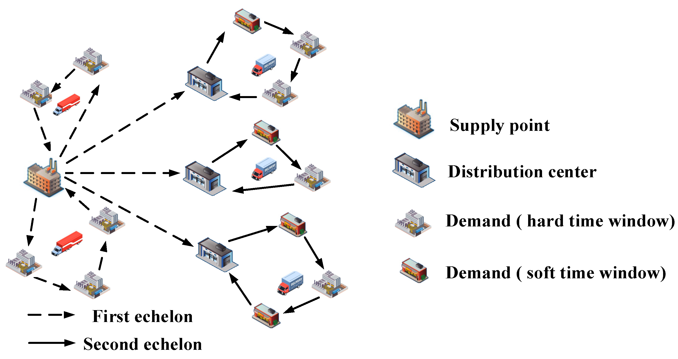
Figure 2.
Schematic Diagram of the Single-Vehicle Exchange Operator.
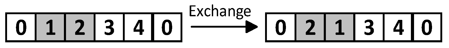
Figure 3.
Schematic Diagram of the Multi-Vehicle Exchange Operator.
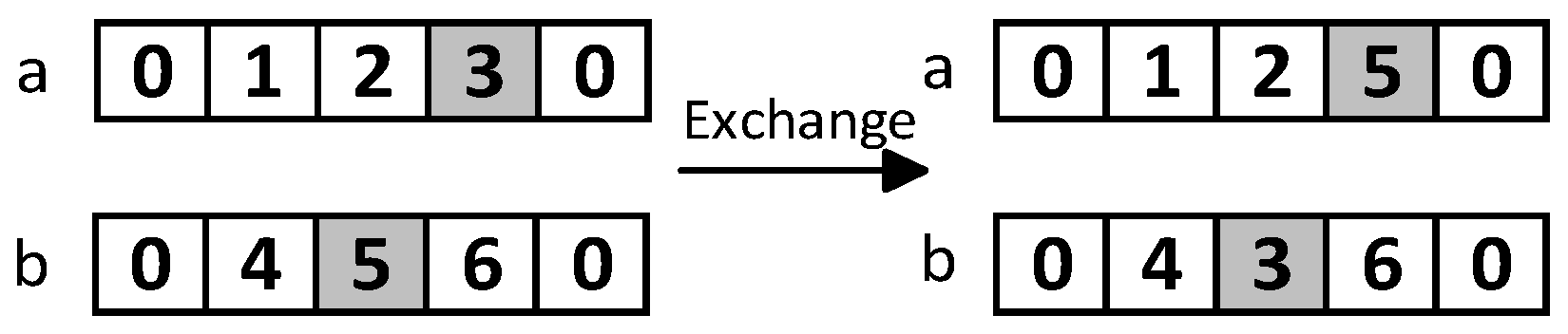
Figure 4.
Space-time Distance-based k-center Greedy Algorithm.
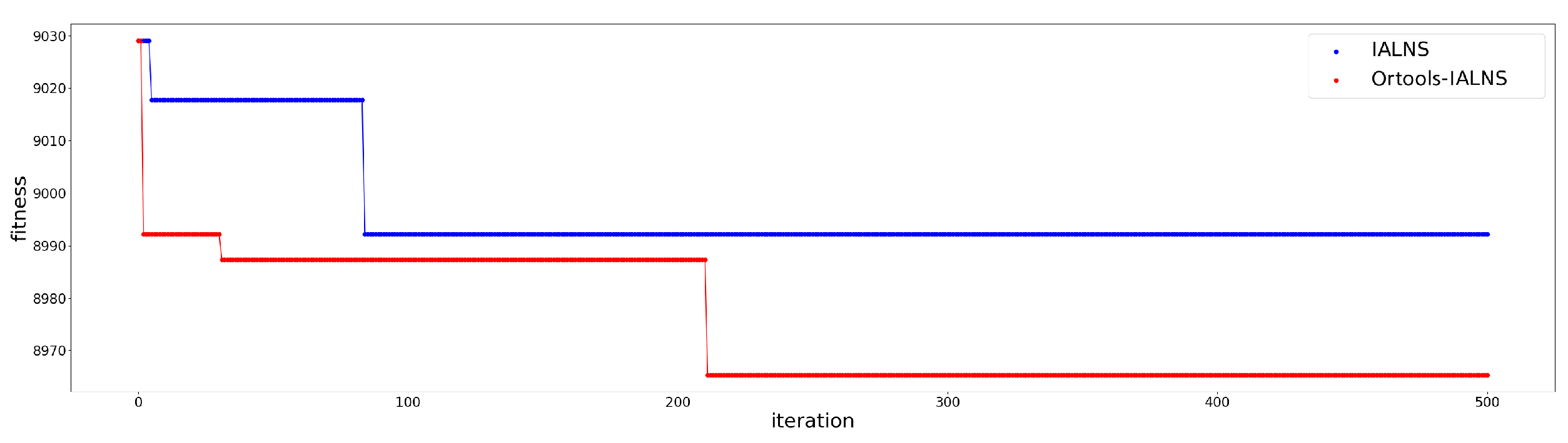
Figure 5.
2-opt Greedy Algorithm.
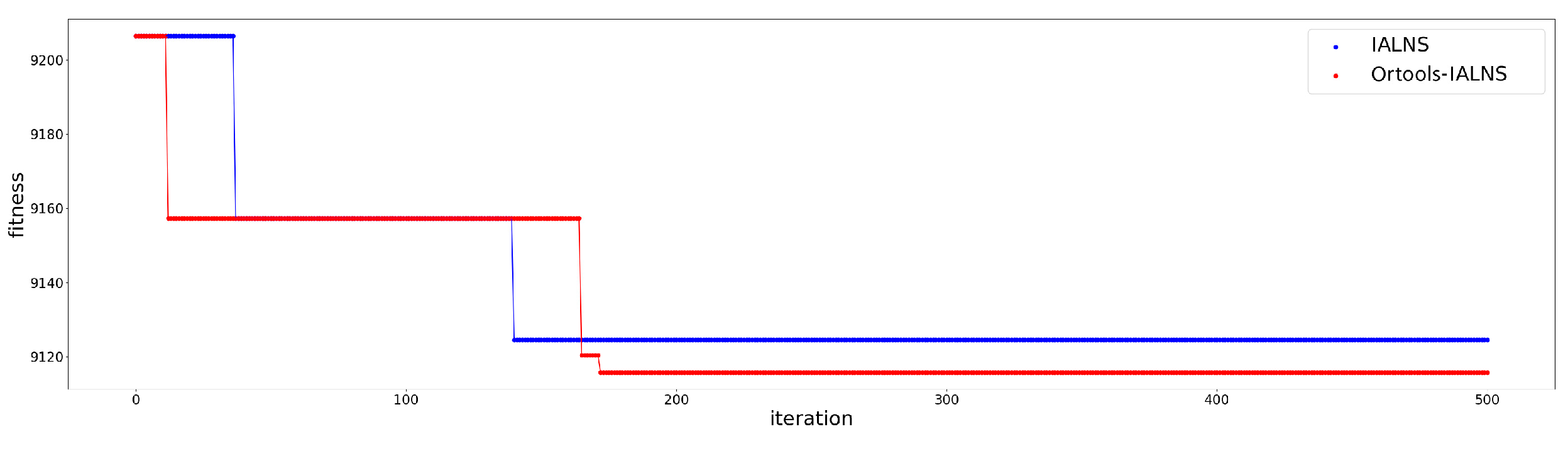
Figure 6.
Greedy Algorithm.
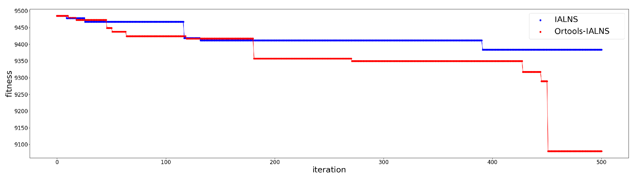

Table 1.
Symbols and Parameters.
| Set | Symbol Explanation |
| Set of all nodes | |
| Supply point nodes | |
| Set of Distribution center nodes | |
| Set of demand points | |
| Subset of demand points with hard time windows(m=1), demand points with soft Time windows(m=2) | |
| Subset of nodes serviceable by primary vehicles | |
| Subset of nodes serviceable by secondary vehicles | |
| Set of primary transport vehicles | |
| Set of secondary transport vehicles | |
| Set | Symbol Explanation |
| Capacity of homogeneous primary transport vehicles | |
| Capacity of homogeneous secondary transport vehicles | |
| Fixed cost of primary vehicles | |
| Fixed cost of secondary vehicles | |
| Distance between node i and node, | |
| Service time at node, | |
| Average speed of primary vehicles | |
| Average speed of secondary vehicles | |
| Loss rate of perishable goods during transportation | |
| Loss rate of perishable goods during service | |
| Unit time penalty cost for early arrival at soft time window customers | |
| Unit time penalty cost for late arrival at soft time window customers | |
| Demand at each demand point | |
| Unit waiting cost for early arrival at demand points with hard time window | |
| Unit refrigerant consumption rate during transport phase for primary vehicles | |
| Unit refrigerant consumption rate during unloading phase for primary vehicles | |
| Unit refrigerant consumption rate during transport phase for secondary vehicles | |
| Unit refrigerant consumption rate during unloading phase for secondary vehicles | |
| Service time window for demand points with hard time window | |
| Expected service time window for demand points with soft time window | |
| Acceptable service time window for demand points with soft time window | |
| Price of perishable products | |
| Unit distance transportation cost for fuel vehicles | |
| Unit distance transportation cost for electric vehicles | |
| Maximum driving distance for electric vehicles | |
| Load of vehicleon, | |
| Arrival time of vehicleat node, | |
| Service start time of vehicleat node, |
Table 2.
Decision Variables.
| Decision Variable | Explanation |
| 1 if vehicletraverses ; 0 otherwise | |
| 1 if the demand at customer node is satisfied through a distribution center; 0 otherwise |
Table 3.
Node Information.
| Node | Coordinates | Demand | Preferred Time Window | Acceptable Time Window | Service Time (min) |
| D1 | 121.519079,31.178838 | 0 | — | — | 0 |
| S1 | 121.336189,31.318649 | 0 | — | — | 0 |
| S2 | 121.361485,31.180489 | 0 | — | — | 0 |
| S3 | 121.351671,31.01652 | 0 | — | — | 0 |
| C1 | 121.375689,31.366831 | 0.6t | 7:30-7:35 | 7:10-9:00 | 15 |
| C2 | 121.455022,31.323576 | 0.4t | 8:00-8:05 | 7:40-9:20 | 10 |
| C3 | 121.427371,31.282269 | 0.4t | 8:30-9:00 | 8:30-9:00 | 10 |
| C4 | 121.232525,31.274027 | 0.8t | 7:30-7:35 | 7:10-8:50 | 20 |
| C5 | 121.464384,31.26076 | 0.4t | 8:30-8:35 | 8:00-10:00 | 10 |
| C6 | 121.351335,31.262449 | 0.8t | 8:40-8:45 | 8:20-10:20 | 20 |
| C7 | 121.391808,31.248767 | 0.8t | 8:00-9:00 | 8:00-9:00 | 20 |
| C8 | 121.422921,31.240309 | 0.6t | 7:30-7:35 | 7:10-8:50 | 15 |
| C9 | 121.33835,31.228173 | 0.6t | 7:50-7:55 | 7:40-9:00 | 15 |
| C10 | 121.371073,31.22393 | 0.4t | 7:50-8:00 | 7:40-9:00 | 10 |
| C11 | 121.201626,31.202598 | 0.6t | 8:00-8:05 | 7:40-9:00 | 15 |
| C12 | 121.437737,31.143082 | 0.4t | 6:20-7:30 | 6:30-7:30 | 10 |
| C13 | 121.391792,31.149528 | 0.6t | 6:00-7:00 | 6:00-7:00 | 15 |
| C14 | 121.447908,31.14241 | 0.6t | 6:30-7:10 | 6:20-7:10 | 15 |
| C15 | 121.318492,31.142219 | 0.6t | 7:30-7:35 | 7:20-9:20 | 15 |
| C16 | 121.28026,31.117884 | 0.4t | 7:30-8:30 | 7:30-8:30 | 10 |
| C17 | 121.320235,31.114561 | 0.6t | 7:30-8:30 | 7:30-8:30 | 15 |
| C18 | 121.413897,31.10436 | 0.6t | 8:20-9:20 | 8:20-9:20 | 15 |
| C19 | 121.510914,31.100481 | 0.6t | 6:00-7:10 | 6:00-7:10 | 15 |
| C20 | 121.589159,31.090836 | 0.8t | 7:00-8:00 | 7:00-8:00 | 20 |
| C21 | 121.411191,31.084089 | 0.4t | 8:20-8:25 | 8:00-9:40 | 10 |
| C22 | 121.347315,31.094539 | 0.8t | 8:30-8:35 | 8:10-9:50 | 20 |
| C23 | 121.270105,31.109855 | 0.6t | 7:30-7:35 | 7:10-8:50 | 15 |
| C24 | 121.228476,31.068138 | 0.6t | 7:40-7:45 | 7:20-9:00 | 15 |
| C25 | 121.456738,31.05216 | 0.4t | 8:00-8:05 | 7:40-9:20 | 10 |
| C26 | 121.24119,31.011107 | 0.8t | 7:50-8:00 | 7:30-8:50 | 20 |
| C27 | 121.420271,31.03132 | 0.4t | 8:00-8:05 | 7:40-9:20 | 10 |
| C28 | 121.518847,31.032595 | 0.4t | 6:30-7:30 | 6:30-7:30 | 10 |
| C29 | 121.440531,30.96813 | 0.6t | 7:50-8:00 | 7:30-8:50 | 15 |
| C30 | 121.492671,31.297665 | 0.6t | 8:20-9:30 | 8:20-9:30 | 15 |
Table 4.
Type 1 Vehicle Parameters.
| Parameter | Value |
| 600 Yuan | |
| 40km/h | |
| 8t | |
| Quantity | 4 |
Table 5.
Type 2 Vehicle Parameters.
| Parameter | Value |
| 250 Yuan | |
| 30km/h | |
| 2.5t | |
| Quantity | 8 |
Table 6.
Parameters Related to Objectives.
| Parameter | Value | Parameter | Value | Parameter | Value | Parameter | Value |
| 0.002 | 40 Yuan/h | 1 Yuan/h | 1.3 Yuan/km | ||||
| 0.003 | 15 Yuan/h | 20000 Yuan/t | 0.8 | ||||
| 40 Yuan/h | 20 Yuan/h | 220km | |||||
| 50 Yuan/h | 10 Yuan/h | 3 Yuan/km |
Table 7.
Cost Comparison of First-Stage Algorithms.
| Algorithm | Fixed | Transport | Refrigeration | Cargo Loss | Penalty | Total Cost | Satisfaction |
| Space-time k-center greedy | 5350 | 743.80 | 311.97 | 2314.95 | 308.34 | 9029.06 | 96.21% |
| 2-opt greedy | 5600 | 734.76 | 308.36 | 2237.11 | 326.21 | 9206.44 | 93.06% |
| Greedy | 5600 | 756.31 | 316.96 | 2354.53 | 457.29 | 9485.09 | 94.65% |
Table 8.
Comparative Results of Second-Stage Algorithms.
| Greedy | 2-opt Greedy | Space-time Distance-based k-center Greedy | ||||||
| Second-Stage Algorithms | IALNS | Ortools-IALNS | IALNS | OrtoolsIALNS | IALNS | Ortools-IALNS | ||
| Fixed | 5600 | 5350 | 5600 | 5600 | 5350 | 5350 | ||
| Transportation | 729.99 | 723.55 | 719.41 | 730.37 | 717.03 | 712.11 | ||
| Refrigeration | 306.45 | 303.87 | 302.22 | 306.60 | 301.26 | 299.29 | ||
| Cargo Loss | 2318.19 | 2331.62 | 2243.49 | 2242.34 | 2296.72 | 2279.75 | ||
| Penalty | 429.09 | 370.67 | 259.45 | 236.44 | 327.19 | 324.13 | ||
| Total | 9383.72 | 9080.01 | 9124.57 | 9115.75 | 8992.20 | 8965.28 | ||
| Satisfaction (%) | 95.1128% | 95.7367% | 95.4544% | 95.4551% | 92.0028% | 92.7767% | ||
Table 9.
Results Under Different Satisfaction Levels.
| Satisfaction Threshold | Fixed | Transportation | Refrigeration | Cargo Loss | Penalty | Total | Actual Satisfaction |
| ≥60% | 5350 | 810.08 | 338.48 | 2331.38 | 436.13 | 9266.07 | 87.55% |
| ≥70% | 5350 | 718.44 | 301.83 | 2295.18 | 484.11 | 9149.56 | 90.26% |
| ≥80% | 5350 | 712.11 | 299.29 | 2279.75 | 324.13 | 8965.28 | 92.78% |
| ≥90% | 5350 | 693.01 | 291.66 | 2229.40 | 374.18 | 8938.25 | 97.42% |
Table 10.
Cost Comparison for a Data Scale of 30 Demand Nodes.
| Data Scale | IALNS | Ortools-IALNS | GAP1/% | GAP2/% |
| C | C | |||
| 30-1:1-6 | 9612.22 | 9232.40 | 3.95% | — |
| 30-0.3:0.7-6 | 8949.70 | 8910.91 | 0.43% | -3.48% |
| 30-0.4:0.6-6 | 8992.20 | 8965.28 | 0.30% | -2.89% |
| 30-0.6:0.4-6 | 9285.10 | 9269.87 | 0.16% | 0.41% |
| 30-0.7:0.3-6 | 10026.69 | 9655.68 | 3.7% | 4.58% |
| 30-1:1-3 | 8395.13 | 8329.34 | 0.78% | — |
| 30-0.3:0.7-3 | 8350.61 | 8310.43 | 0.48% | -0.23% |
| 30-0.4:0.6-3 | 8342.02 | 8319.95 | 0.26% | -0.11% |
| 30-0.6:0.4-3 | 8380.33 | 8361.29 | 0.22% | 0.38% |
| 30-0.7:0.3-3 | 9754.01 | 8910.84 | 8.64% | 6.98% |
Table 11.
Cost Comparison for a Data Scale of 40 Demand Nodes.
| Data Scale | IALNS | Ortools-IALNS | GAP1/% | GAP2/% |
| C | C | |||
| 40-1:1-6 | 11442.61 | 11206.45 | 2.06% | — |
| 40-0.3:0.7-6 | 11168.27 | 10979.78 | 1.69% | -2.02% |
| 40-0.4:0.6-6 | 11327.20 | 11106.72 | 1.95% | -0.89% |
| 40-0.6:0.4-6 | 11561.03 | 11237.28 | 2.80% | 0.28% |
| 40-0.7:0.3-6 | 11495.71 | 11288.33 | 1.80% | 0.73% |
| 40-1:1-3 | 10120.82 | 10039.85 | 0.80% | — |
| 40-0.3:0.7-3 | 10036.88 | 9920.34 | 1.16% | -1.19% |
| 40-0.4:0.6-3 | 10037.74 | 10026.90 | 0.11% | -0.13% |
| 40-0.6:0.4-3 | 10218.74 | 10139.85 | 0.77% | 0.99% |
| 40-0.7:0.3-3 | 11073.03 | 10973.10 | 0.90% | 9.30% |
Table 12.
Cost Comparison for a Data Scale of 50 Demand Nodes.
| Data Scale | IALNS | Ortools-IALNS | GAP1/% | GAP2/% |
| C | C | |||
| 50-1:1-6 | 13479.45 | 13135.93 | 2.55% | — |
| 50-0.3:0.7-6 | 13118.99 | 12658.86 | 3.51% | -3.63% |
| 50-0.4:0.6-6 | 13259.92 | 12698.76 | 4.23% | -3.33% |
| 50-0.6:0.4-6 | 13776.39 | 13150.06 | 4.55% | 0.11% |
| 50-0.7:0.3-6 | 13218.68 | 13165.01 | 0.41% | 0.22% |
| 50-1:1-3 | 13290.33 | 12221.38 | 8.04% | — |
| 50-0.3:0.7-3 | 11577.62 | 11338.74 | 2.06% | -7.22% |
| 50-0.4:0.6-3 | 11849.68 | 11659.99 | 1.60% | -4.59% |
| 50-0.6:0.4-3 | 14195.33 | 12843.36 | 9.52% | 5.09% |
| 50-0.7:0.3-3 | 13617.69 | 13045.75 | 4.20% | 6.75% |
Disclaimer/Publisher’s Note: The statements, opinions and data contained in all publications are solely those of the individual author(s) and contributor(s) and not of MDPI and/or the editor(s). MDPI and/or the editor(s) disclaim responsibility for any injury to people or property resulting from any ideas, methods, instructions or products referred to in the content. |
© 2024 by the authors. Licensee MDPI, Basel, Switzerland. This article is an open access article distributed under the terms and conditions of the Creative Commons Attribution (CC BY) license (http://creativecommons.org/licenses/by/4.0/).
Copyright: This open access article is published under a Creative Commons CC BY 4.0 license, which permit the free download, distribution, and reuse, provided that the author and preprint are cited in any reuse.


