
Submitted:
19 November 2024
Posted:
19 November 2024
You are already at the latest version
Abstract
Rural infrastructure is an important foundation for achieving sustainable rural development. To effectively formulate policies for rural infrastructure, it is crucial to evaluate the benefits of rural infrastructure investment (RII) using a systematic method. This study aims to conduct a systematic analysis of the income-increasing effect of RII from a multi-dimensional perspective, and provide a reference for developing countries to adjust and improve rural infrastructure policies. For this purpose, this study has utilized 15 years of data in China to analyze the income-increasing effect of RII from three dimensions: structure, spatiality, and heterogeneity. The results indicate that: (1) In terms of structure, both living infrastructure investment (LII) and production infrastructure investment (PII) promote wage income. PII has the increasing effect on non-wage income, but the increasing effect of LII on non-wage income is not evident. Meanwhile, the income-increasing effect of RII for high-income groups is larger than that for low-income groups. (2) In terms of spatiality, RII has a spatial spillover effect, which increases villagers' income in neighboring areas. From the perspective of spatial effect decomposition, the indirect effect of RII even exceeds the direct effect. (3) In terms of heterogeneity, the increase in the level of job-related migration inhibits the income-increasing effect of LII, but promotes the income-increasing effect of PII; the improvement in education level promotes the income-increasing effect of LII, but inhibits the income-increasing effect of PII.
Keywords:
rural infrastructure
; income
; structure
; spatiality
; heterogeneity
; China
1. Introduction
Infrastructure investment is one of the United Nations' Sustainable Development Goals. Economic growth, social development and risk resilience rely heavily on infrastructure investment, which is highly significant for promoting sustainable development worldwide. The World Bank has also been assisting developing countries in building public infrastructure to advance inclusive growth, create jobs and stimulate sustainable infrastructure development. Despite these observations, China still confronts a serious rural infrastructure gap. There is still a considerable amount of debt in rural infrastructure. The supply of hardened roads, water supply and drainage, and natural gas facilities in villages is relatively inadequate. Rural social security and comprehensive service facilities are conspicuously lacking. The task of rural sanitary toilet transformation and domestic sewage and garbage treatment remains burdensome. The infrastructure such as water, electricity and roads of some cultivated land is insufficient, and the disaster resistance ability is poor. Rural infrastructure challenges continue to be an important factor restricting the sustainable development of rural areas.
China is currently implementing the rural revitalization strategy. How to broaden villagers' income channels and promote common prosperity constitutes an important issue for China to achieve comprehensive rural revitalization in the future. The most difficult and arduous task in fully realizing China's modernization remains in the countryside. To effectively formulate rural infrastructure policies, it is essential to adopt a systematic method to evaluate the benefits of rural infrastructure investment (RII). Rural infrastructure frequently adopted a top-down investment decision, which may result in the coexistence of insufficient and oversupply of rural infrastructure in space, ultimately manifesting as low efficiency of rural infrastructure construction and significantly diminished comprehensive benefits. Meanwhile, in the context of the escalating hollowing out of rural areas, scholars have gradually focused on for whom rural infrastructure is intended, and the effect of RII on increasing villagers' income has been queried. Consequently, this study undertook a systematic analysis of the income-increasing effect of RII based on a multi-dimensional perspective of structure, spatiality and heterogeneity, combined with China's rural infrastructure macro-investment data. This study aims to offer decision-making support for enhancing China's RII policies, and furnish some policy inspiration for the rural revitalization path of other developing countries.
2. Literature Review
John Maynard Keynes stated in The General Theory of Employment, Interest Rates and Money that infrastructure indirectly influences income growth. In the event of economic depression and low market efficiency, high public spending stimulates high level of employment[1]. The notion that strengthening public infrastructure investment is a key factor in long-term sustainable growth and income generation has become a mainstream view in the literature[2,3]. RII has an income-increasing effect by directly reducing villagers' production costs and enhancing their productivity[4]. Rural infrastructure has a trickle-down effect, whereby it has an influence on economic growth and thus indirectly on income[5,6]. Rural infrastructure has a positive effect on enhancing the life quality of the rural poor and alleviating poverty[7,8,9]. Rural infrastructure enhances the availability of basic public services[10], such as health, education, and employment[11,12,13]. Meanwhile, studies have indicated that different types of rural infrastructure have income-increasing effect. Agricultural distribution infrastructure significantly narrows the rural-urban income gap and have a poverty-reducing effect, but there are regional disparities[14]. Investment in rural power and irrigation facilities significantly boosts villagers' farm income[15] . Rural transport infrastructure facilitates rural labor mobility and increase the income of villagers, especially those with low agricultural and business income[16]. The impact of rural Internet infrastructure on digital financial inclusion is greater in areas with higher level of education[17]. Rural water supply infrastructure contributes to coordinated urban-rural development and increase with investment equity[18].
But contrary to the above, the micro-school of thought, based on case studies and large datasets, considered infrastructure investments to be extremely poor in terms of financial, environmental and social performance[19]. Improvements in rural infrastructure contribute to urbanization, but they also result in a reduction of productive capital and quality labor in rural areas. In such “empty villages”, RII don't have the income-increasing effect, and the rural poor might sink into greater poverty[20]. Meanwhile, there are structural differences in rural infrastructure regarding villagers' income. In Nepal rural road infrastructure doesn't increase crop income, road infrastructure in the Philippines reduces the average consumption expenditure of the poor and widens income inequality[21]. China's electricity transmission infrastructure increases villagers' income but also aggravates rural-urban income inequality[22]. Different research findings have given rise to unclear implications for government policies in RII.
Despite the progress achieved in research on the income-increasing effect of rural infrastructure, a number of limitations remain. Previous research focused on reflecting the differences in income-increasing effect based on the physical stock of rural infrastructure. Although the physical stock indicator directly reflects the actual situation of RII, it is challenging to sum up the physical stocks of different types of infrastructure. Generally, rural infrastructure can be classified into living infrastructure and production infrastructure. Living infrastructure encompasses roads and bridges, water supply, drainage, gas, landscaping, etc.; Production infrastructure encompasses houses and buildings utilized for agricultural production, large and medium-sized iron and wooden farm tools, and agricultural machinery. Since there is an evident distortion in the capital investment structure of rural infrastructure, which emphasizes living infrastructure and neglects production infrastructure, it might be more practical to explore the differences in the income-increasing effect of rural infrastructure based on the classification of capital investment. Most existing studies commence from a single perspective of income-increasing, and lack a systematic investigation of the income-increasing effect of RII from a multidimensional perspective. The novelty of this study resides in the systematic exploration of the income-increasing mechanism and effect from the perspectives of structure, spatiality and heterogeneity.
3. Theoretical Analysis and Research Hypotheses
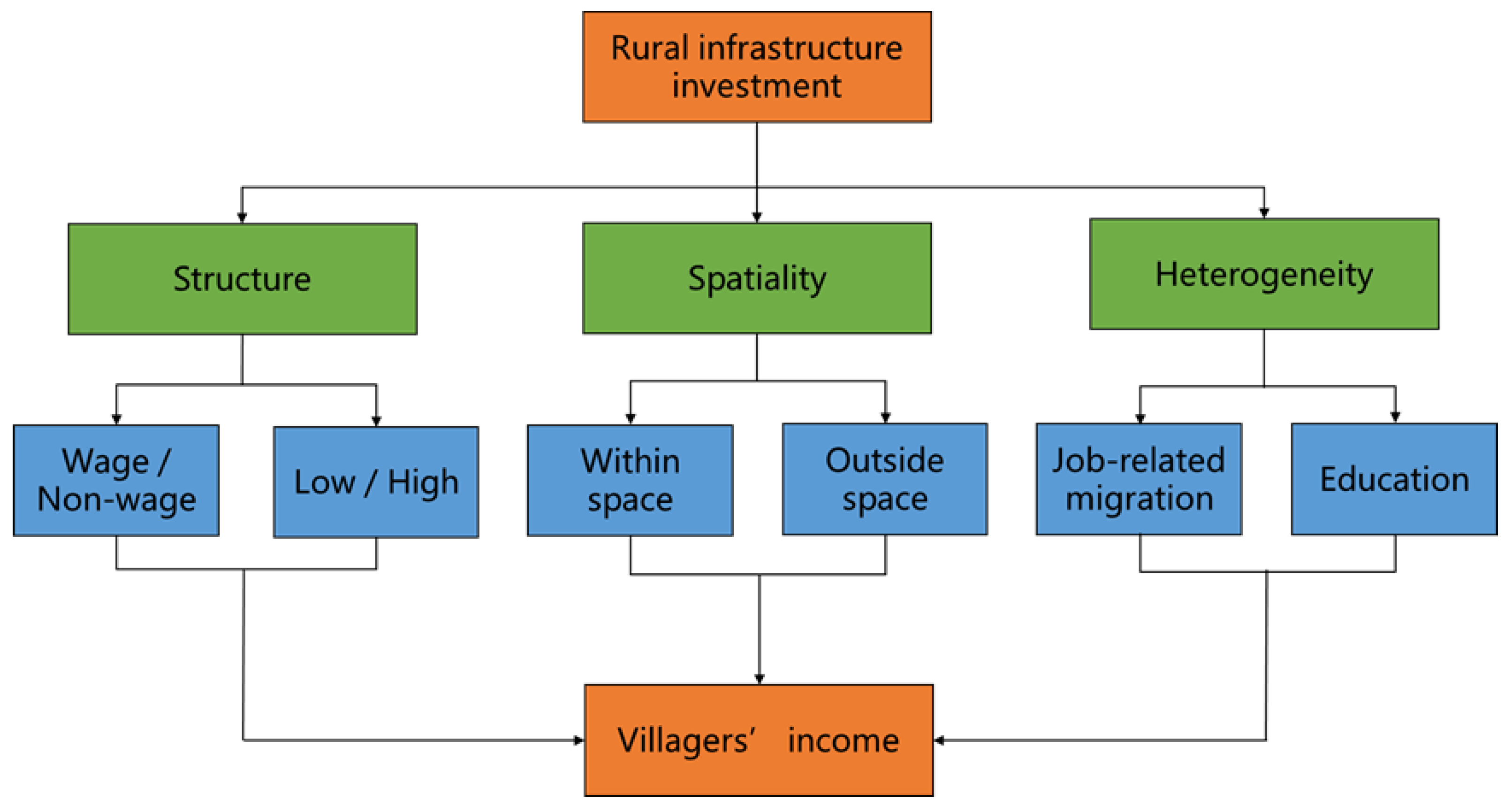
3.1. Structure
The structural differences in the income-increasing effect of RII mainly lie between wage and non-wage incomes, and between high-income and low-income villagers. On the one hand, RII has different mechanisms of action regarding villagers' wage and non-wage incomes. In response to wage income, LII enhances villagers' welfare and entrepreneurial basis mainly through indirect effect. LII reduces the mobility and information exchange costs for villagers, alleviates the friction in the job market, and makes it easier for more villagers to go out to work. LII stimulates the development of new local rural industries, where villagers can be matched with suitable jobs without having to travel far from home. Industries derived from LII encompass secondary and tertiary industries, such as logistics, packaging, processing, and tourism services, which further increase villagers' wage income. PII reduces the amount of time villagers spend on agriculture labor, providing more off-farm employment opportunities and increasing wage income. In response to non-wage income, LII and PII has increased villagers' property income, such as house rent and rent from the transfer of land management rights. PII directly serves as an input factor for agricultural production, increasing agricultural output. PII has facilitated the use of data, agricultural technology equipment, etc. in agricultural production and management, further increasing operating income. Rural areas with good living infrastructure conditions are more likely to attract production subsidies, further increasing transfer income.
On the other hand, who benefits from rural infrastructure, high-income villagers or low-income villagers, is a question worthy of consideration. Rural infrastructure brings more changes in production technology and imposes higher demands on villagers' initiative. Since there is a significant overlap between low-income villagers and those who have difficulty using technology, RII may be more beneficial to high-income villagers. Generally, high-income villagers are highly educated, and enhance their information search and communication abilities through rural infrastructure, thereby enjoying the benefits of rural infrastructure to a greater extent. However, due to the limitations of their education, low-income villagers frequently find it challenging to utilize technical rural infrastructure to develop production or find non-agricultural jobs. Low-income villagers are unable to enhance the scientific nature of production decisions and expand the value chain. Therefore, high-income villagers extract more resources with the assistance of rural infrastructure, thereby forming a Matthew effect of "the rich get richer".
Hypothesis 1: RII increases villagers' income, but there are disparities in the impact of LII and PII on villagers' wage and non-wage incomes, as well as on high-income and low-income villagers.
3.2. Spatiality
Villagers' income tends to be spatially distributed. Low-income rural populations are concentrated in remote rural areas, having strong spatial correlations with the level of rural public goods provision, resource endowments and other factors. Poor location conditions and backward infrastructure result in weak industry-led capacity, and under the cumulative effect of this non-linear negative cycle, a spatial low-income trap is formed. At the micro level, the difficulty in increasing villagers' income is the outcome of a combination of villagers' endowment and geographical endowment; At the macro level, the difficulty of increasing villagers' income is a state of dysfunctional coupling among the dimensions of people, industry, and land within a given space and time. With the advancement of the times, villagers are no longer isolated spatially. They are gradually integrated into the marketization process and move freely between urban and rural areas. This movement constitutes an important way for villagers to get rid of poverty. The urbanization process has rendered villagers' livelihoods increasingly dependent on non-agricultural industries. Villagers' consumption patterns, identity, and social mobility have gradually become more in alignment with cities. The economy and ecology have broken through the original spatial limitations, and the intensity, complexity and diversity of connections have increased[23].
Rural infrastructure creates opportunities that no longer rely on local system for services or livelihoods, but can be sourced to more distant geographical areas[24]. Infrastructure such as rural roads integrates labor markets across space and enhances the mobility of villagers[25]. The scale and structural characteristics of fiscal expenditure among governments exhibit a clear degree of mutual imitation strategic interaction. Provinces with better rural infrastructure development prompt neighboring provinces to follow suit[26]. RII in the region expands the scope and efficiency of agricultural product transactions in adjacent areas, and brings larger trading markets to adjacent areas. As a result, RII boosts villagers' income growth. The effect of rural infrastructure on increasing villagers' income is converging, resulting in spatial correlation in rural infrastructure, namely, spatial spillover effect.
Hypothesis 2: RII exerts a spatial spillover effect on increasing villagers’ income.
3.3. Heterogeneity
The essence of rural labor transfer is the choice made after comparing the economic interests of different sectors and those of urban and rural public services. In urban areas, the combination of superior educational resources, convenient transportation and information networks creates a good environment for residents to participate in higher-quality education or skills training. Coupled with the significant disparity between non-agricultural and agricultural incomes, a large number of rural populations have been attracted. Due to the job-related migration of rural labor, the hollowing out of some rural populations is inevitable. A large number of "empty houses" have emerged in rural areas. A large amount of funds has been invested in rural infrastructure construction, which is facing the problem of "for whom it is built". In areas where the degree of job-related migration is large, the marginal effect of increased income from LII enjoyed by villagers who go to cities for employment declines, which weakens the income-increasing effect brought about by the LII. PII reduces villagers' agricultural production costs, enabling them to have more time to engage in non-agricultural jobs. In areas with a large degree of job-related migration, the income-increasing effect brought by PII is magnified.
Compared with migrant workers in cities, although the number of those who are employed locally or return to their hometowns for employment and entrepreneurship is relatively small, they possess broader academic qualifications and vision, and exert a greater role in increasing income through rural infrastructure. The education level of the population has a further influence on the income-increasing effect through its impact on the utilization efficiency of rural infrastructure. In areas with high level of education, villagers tend to have more employment opportunities, and the income-increasing effect of LII is magnified. However, villagers with higher level of education are more inclined to work outside their hometowns. Villagers enhance their non-agricultural professional skills through formal education and skills training, thereby driving the growth of their income. In areas with high level of education, the marginal effect of increased income from PII enjoyed by villagers declines, and the income-increasing effect of PII is diminished.
Hypothesis 3: Job-related migration and education level have a moderating effect on the income-increasing effect of RII.
Figure 1.
The multi-dimensional impact of rural infrastructure investment on villagers’ income.
4. Materials and Methods
4.1. Variables
- Explained variables. This study employed villagers’ income, wage income, and non-wage income in each province as explained variables. Non-wage income comprised villagers’ business income, transfer income, and property income.
- Explanatory variables. This study categorized rural infrastructure into LII and PII. LII pertained to infrastructure investment in water, gas, heating, roads, drainage, landscaping, environmental sanitation, etc. in rural areas; PII referred to agricultural production construction projects such as agriculture, forestry and pasture, the purchase of machinery and equipment for agricultural production, as well as investment in farmland construction projects, irrigation, drainage and other small-scale water conservancy projects in rural townships, villages and groups. The perpetual inventory method was utilized to calculate RII, and the formula was as follows:
- 3.
- Control variables. In addition to the two core explanatory variables of LII and PII, this study also employed control variables such as job-related migration level, education level, economic development level, urbanization level, cultivated land endowment, openness level, and agricultural development level, referring to the practices of existing literature. Job-related migration level was expressed as the proportion of migrant labors to the aggregate labors; Education level was expressed as the average years of the villagers’ education; Economic development level was expressed as per capita comparable Gross Domestic Product (GDP); Urbanization level was expressed as the urbanization rate; Cultivated land endowment was expressed as the ratio of family-operated cultivated land area to the number of rural population; Openness level was expressed as the proportion of the total import and export volume to the GDP; Agricultural development level was expressed as the proportion of gross agricultural production to the GDP.
4.2. Data
The data of this study were the panel data of 30 provinces in inland China except Tibet from 2007 to 2022. The data came from the annual China Urban and Rural Construction Statistical Yearbook, China Statistical Yearbook, China Population and Employment Statistical Yearbook, China Rural Policy and Reform Statistical Bulletin and provincial statistical yearbooks. The descriptive statistics of each variable are shown in Table 1.
4.3. Models
Benchmark model. Considering only the structure of villagers' wage income and non-wage income, as well as the heterogeneity of job-related migration and education level, the benchmark model was set as follows:
Where represented villagers' income, including villagers' wage income and non-wage income ; and represented LII and PII; represented a series of control variables; was the residual term; the subscript represented the province, the subscript represented the year, and , , and were the corresponding variable coefficients. This study employed a fixed effect model. To eliminate possible endogenous effect, the core explanatory variables were lagged by one period.
- 4.
- Quantile regression model. The quantile regression model compares the influence of the independent variable on the dependent variable at different quantile points[28]. When the explanatory variable has varying effects on the explained variable at different quantiles, such as left skewness or right skewness, quantile regression captures the tail characteristics of the distribution. It was utilized to examine the differences in the income-increasing effect of RII between high-income villagers and low-income villagers. For a population of random variables y, the general linear conditional quantile function for the τ-th quantile was:
- 5.
- Spatial panel regression model. The spatial panel regression model includes the Spatial Autoregression Model (SAR), the Spatial Durbin Model (SDM), and the Spatial Error Model (SEM). They were used to consider the spatial spillover effect of RII. The general expressions were:
5. Results
5.1. Analysis of Spatial Agglomeration Characteristics
5.1.1. Spatial Static Distribution
In order to explore the spatial distribution of rural infrastructure and villagers' income, this study selected two years, 2007 and 2022, and divided the variables into five categories by using the natural breakpoint method. As can be seen from Figure 2 (a) and (b), regions in China with less LII presented a clear agglomeration pattern. In 2007, regions with less LII were concentrated in the southwest region of China and provinces such as Gansu, Inner Mongolia, Hebei, and Henan. In 2022, provinces with less LII were concentrated in Hebei, Henan, and Heilongjiang. As can be seen from Figure 2 (c) and (d), regions in China with more PII presented a clear agglomeration pattern. In 2007, regions with more PII were concentrated in northern provinces such as Heilongjiang, Jilin, Liaoning, Inner Mongolia, and Xinjiang. In 2022, regions with more PII were concentrated in northern provinces such as Heilongjiang, Inner Mongolia, and Shaanxi. As can be seen from Figure 2 (e) and (f), villagers' income presented a clear agglomeration pattern. In 2007 and 2022, provinces with higher villagers' income were concentrated in China's eastern coastal areas, while provinces with lower villagers' income were concentrated in the western regions of China.
5.1.2. Spatial Dynamic Distribution
As can be seen from Figure 3 and Table 2, from 2007 to 2022, the focus of LII gradually shifted from the northeast to the southwest. The flattened standard deviation ellipse first presented a significant increase and then slightly decreased, indicating that the concentration of China's LII in the "northeast-southwest" direction increased and then slightly weakened. The area of the standard deviation ellipse has continuously increased, indicating that the scope of LII in China has continued to expand. The focus of PII shifted from the northwest to the southeast and then from the northeast to the southwest. The flatness of the standard deviation ellipse first increased and then decreased. The focus of LII in the "northeast-southwest" direction in China increased and then weakened. The area of the standard deviation ellipse first increased and then decreased, indicating that the scope of PII first increased and then weakened. The focus of villagers' income gradually shifted from the northeast to the southwest, and the flatness of the standard deviation ellipse first increased and then decreased, which was consistent with the change directions of LII and PII, indicating that villagers' income had obvious spatial correlation with RII.
5.2. Structure of RII
According to the econometric results in Table 3, it can be observed that both LII and PII have a significant income-increasing effect. For every 1-yuan increase in LII, villagers' income increased by 0.004%, and for every 1-yuan increase in PII, villagers' income increased by 4.6%. From the perspective of income decomposition, both LII and PII had the increasing effect on wage income, and PII had the increasing effect on non-wage income, but the increasing effect of LII on non-wage income was not significant. The level of job-related migration and agricultural development had a significant positive effect on villagers' income and wage income. The possible reason was that in provinces with a higher level of agricultural development, agricultural competition was more intense, and more people chose to work outside the provinces. At the same time, migrant workers had more non-agricultural employment opportunities. The level of education, economic development and urbanization had a significant positive effect on villagers' income, wage income and non-wage income, indicating that the higher the level of education, economic development and urbanization, the higher the villagers' income. Cultivated land endowment had a significant negative effect on villagers' income and wage income, but had a significant positive effect on non-wage income, indicating that regions with better cultivated land endowment increased the opportunity cost of villagers working outside the home, while bringing more favorable conditions for agricultural production, reducing villagers' wage income and increasing villagers' non-wage income. The level of openness to the outside world had a significant negative effect on villagers' income and wage income. The possible reason was that the higher the degree of openness, the more intense the employment competition, which was not conducive to the increase of villagers' wage income in the region.
This study employed the quantile regression method to analyze the differential impact of RII on villagers with different income levels, and selected five quantiles of 10%, 25%, 50%, 75%, and 90%, respectively representing the low-income group, the lower-middle-income group, the middle-income group, the higher-middle-income group, and the high-income group. Table 4 presents the results of the quantile regression.
From the quantile regression results in Table 4, it is observed that at the quantile level ranging from 25% to 90%, both LII and PII had an effect of increasing villagers' income. Further comparison of the regression coefficients indicated that as the percentile of villagers' income levels rose, the marginal effects of LII and PII on villagers' income demonstrated an upward trend. From the lower-middle-income groups to the high-income groups, for every unit increase in LII, the growth trend of villagers' income levels was 0.003%→0.004%→0.005%→0.007%, and for every unit increase in PII, the growth trend of villagers' income levels was 3.30%→4.64%→5.76%→6.81%, suggesting that RII would be more beneficial to high-income villagers.
5.3. Spatiality of RII
This study employed the SAR, SEM and SDM to estimate and compare the samples. First, the optimal spatial econometric model needed to be determined. The estimation strategy adopted in this study was to conduct likelihood ratio (LR) test and Akaike information criterion test (AIC). The relevant test results are presented in Table 5. The LR test indicated that the SDM cannot be degenerated into the SEM model and the SAR model, so the SDM was utilized. The AIC test also discovered that the SDM was optimal. After the Hausman test, it was supported to use the fixed effect model, so this study employed the fixed effect model for analysis.
This study decomposed the spatial total effect of RII on villagers' income into the direct effect and the indirect effect. The direct effect was employed to capture the impact of influencing factors on the region, and the indirect effect was employed to capture the impact on neighboring regions. As can be seen from Table 6, the impact of LII and PII on villagers' income presented a positive total effect. LII and PII not only exerted the income-increasing effect on villagers in the local area, but also exerted the spatial spillover effect. For every 1-yuan increase in LII, villagers' income in neighboring areas increased by 0.006%, and for every 1-yuan increase in PII, villagers' income in neighboring areas increased by 3.52%. From the perspective of effect decomposition, the indirect effect brought about by RII was higher than the direct effect.
5.4. Heterogeneity of RII
This study employed the national average as the line to divide provinces into those with low and high level of job-related migration, and those with low and high level of education. As can be seen from Table 7, in provinces with low job-related migration level, for every 1-yuan increase in LII, villagers' income increased by 0.005%, and for every 1-yuan increase in PII, villagers' income increased by 3.72%; In provinces with high job-related migration level, the income-increasing effect of LII was insignificant. For every 1-yuan increase in PII, villagers' income increased by 4.14%. This indicated that the increase in the level of job-related migration had suppressed the income-increasing effect of LII, but promoted the income-increasing effect of PII. In provinces with high level of education, for every 1-yuan increase in LII, villagers' income increased by 0.004%, and for every 1-yuan increase in PII, villagers' income increased by 3.15%; In provinces with low level of education, the income-increasing effect of LII was insignificant. For every 1-yuan increase in in PII, villagers' income increased by 8.35%. This indicated that the improvement of education level has promoted the income-increasing effect of LII, but inhibited the income-increasing effect of PII.
6. Results
In the context of developing countries achieving sustainable development goals, the exploration of the income-increasing effect of RII is crucial for increasing villagers' income and achieving common prosperity. This study estimated the capital stock of China's provincial RII from 2007 to 2022 based on the perpetual stock method and analyzed the income-increasing effect of RII from the three-dimensional perspectives of structure, spatiality, and heterogeneity. The research results show that: (1) in terms of structure, both LII and PII promote wage income. PII has the increasing effect on non-wage income, but the increasing effect of LII on non-wage income is not evident. Meanwhile, the income-increasing effect of RII for high-income groups is larger than that for low-income groups. (2) In terms of spatiality, RII has a spatial spillover effect, which increases villagers' income in neighboring areas. From the perspective of spatial effect decomposition, the indirect effect of RII even exceeds the direct effect. (3) In terms of heterogeneity, the increase in the level of job-related migration inhibits the income-increasing effect of LII, but promotes the income-increasing effect of PII; the improvement in education level promotes the income-increasing effect of LII, but inhibits the income-increasing effect of PII.
Since the income-increasing effect of RII has structural, spatial and heterogeneous influences, developing countries take the following into consideration when formulating and implementing policies to strengthen RII and increase villagers' income: (1) Given that the income-increasing effect of RII on high-income villagers is greater than that on low-income villagers, support and assistance to vulnerable groups in rural areas should be enhanced, more inclusive and equitable sustainable development strategies should be adopted, education coverage and non-agricultural employment training for vulnerable groups in rural areas should be strengthened, the driving effect brought about by RII should be expanded, and opportunities for vulnerable groups to share the dividends of rural infrastructure construction should be increased. (2) Given the spatial nature of RII, in China, villagers in economically underdeveloped areas rely more on non-wage income, but the role of LII in promoting non-wage income is not obvious, indicating that LII in underdeveloped areas is still lagging. The regional layout of rural infrastructure should be optimized by the government. RII should be focused on underdeveloped areas. The shortcomings of rural infrastructure should be targeted. The focus and timing of rural infrastructure construction should be determined in accordance with local conditions based on regional human, financial, material, and other factors, so as to promote the coordinated development of rural infrastructure in this region and neighboring areas. (3) Given that both job-related migration and education level have an impact on the income-increasing effect of RII, Urban and rural population mobility and differences in education level should be taken into account. The development positioning of villages should be reasonably determined. RII should be promoted to adapt to changes in rural job-related migration and education level. The problem of "for whom and by whom" rural infrastructure is built should be solved.
Author Contributions
Conceptualization: S.Y. and X.W.; methodology, S.Y.; software, S.Y.; validation, S.Y.; formal analysis, S.Y.; investigation, X.W.; resources, S.Y.; data curation, S.Y.; writing—Original draft preparation, S.Y.; writing—review and editing, S.Y.; visualization, S.Y.; supervision, X.W.; project administration, S.Y.; funding acquisition, X.W. All authors have read and agreed to the published version of the manuscript.
Funding
This work was co-funded by the Science and Technology Innovation Team Project grant (CXTD-2024-04), the Talent Project grant (QNYC-2024-06), and the Independent Research and Development Project (QD202404) of the Academy of Agricultural Planning and Engineering.
Institutional Review Board Statement
Not applicable.
Data Availability Statement
The data presented in this study are available on request from the first author.
Acknowledgments
We would like to express our appreciation to the anonymous reviewers for the insightful comments that improved this manuscript.
Conflicts of Interest
The authors declare no conflict of interest.
References
- Haberler, G. The Place of the General Theory of Employment, Interest, and Money in the History of Economic Thought. Rev. Econ. Stat. 1946, 28, 187. [Google Scholar] [CrossRef]
- Chakamera, C.; Alagidede, P. The nexus between infrastructure (quantity and quality) and economic growth in Sub Saharan Africa. Int. Rev. Appl. Econ. 2017, 32, 641–672. [Google Scholar] [CrossRef]
- Dah, O.; Bassolet, T.B. Agricultural infrastructure public financing towards rural poverty alleviation: evidence from West African Economic and Monetary Union (WAEMU) States. SN Bus. Econ. 2021, 1, 39. [Google Scholar] [CrossRef]
- Chotia, V.; Rao, N. Investigating the interlinkages between infrastructure development, poverty and rural–urban income inequality: Evidence from BRICS nations. Studies in Economics and Finance 2017, 34, 466–484. [Google Scholar] [CrossRef]
- Qin, X.; Wu, H.; Shan, T. Rural infrastructure and poverty in China. PLOS ONE 2022, 17, e0266528. [Google Scholar] [CrossRef]
- Hulten, C.R.; Bennathan, E.; Srinivasan, S. Infrastructure, Externalities, and Economic Development: A Study of the Indian Manufacturing Industry. World Bank Econ. Rev. 2006, 20, 291–308. [Google Scholar] [CrossRef]
- Akbar, M.; Abdullah; Naveed, A.; Syed, S.H. Does an Improvement in Rural Infrastructure Contribute to Alleviate Poverty in Pakistan? A Spatial Econometric Analysis. Soc. Indic. Res. 2021, 162, 475–499. [Google Scholar] [CrossRef]
- Ogun, T.P. Infrastructure and Poverty Reduction: Implications for Urban Development in Nigeria. Urban Forum 2010, 21, 249–266. [Google Scholar] [CrossRef]
- Zhang, L.; Zhuang, Y.; Ding, Y.; Liu, Z. Infrastructure and poverty reduction: Assessing the dynamic impact of Chinese infrastructure investment in sub-Saharan Africa. J. Asian Econ. 2023, 84, 101573. [Google Scholar] [CrossRef]
- Sewell, S.; Desai, S.; Mutsaa, E.; Lottering, R. A comparative study of community perceptions regarding the role of roads as a poverty alleviation strategy in rural areas. Journal of rural studies 2019, 71, 73–84. [Google Scholar] [CrossRef]
- Oisasoje, O.M.; Ojeifo, S.A. The role of public infrastructure in poverty reduction in the rural areas of Edo State, Nigeria. Research on Humanities and Social Sciences 2012, 2, 109–120. [Google Scholar]
- Medeiros, V.; Ribeiro, R.S.M.; Amaral, P.V.M.D. Infrastructure and household poverty in Brazil: A regional approach using multilevel models. World Dev. 2021, 137, 105118. [Google Scholar] [CrossRef]
- Wan, G.; Wang, C.; Zhang, X.; Zuo, C. Income inequality effect of public utility infrastructure: Evidence from rural China. World Dev. 2024, 179, 106594. [Google Scholar] [CrossRef]
- Liu, X.; Zeng, F. Poverty Reduction in China: Does the Agricultural Products Circulation Infrastructure Matter in Rural and Urban Areas? Agriculture 2022, 12, 1208. [Google Scholar] [CrossRef]
- Xiao, H.; Zheng, X.; Xie, L. Promoting pro-poor growth through infrastructure investment: Evidence from the Targeted Poverty Alleviation program in China. China Econ. Rev. 2021, 71, 101729. [Google Scholar] [CrossRef]
- Lu, H.; Zhao, P.; Hu, H.; Zeng, L.; Wu, K.S.; Lv, D. Transport infrastructure and urban-rural income disparity: A municipal-level analysis in China. J. Transp. Geogr. 2022, 99, 103292. [Google Scholar] [CrossRef]
- Niu, G.; Jin, X.; Wang, Q.; Zhou, Y. Broadband infrastructure and digital financial inclusion in rural China. China Econ. Rev. 2022, 76, 101853. [Google Scholar] [CrossRef]
- Shijie, J.; Liyin, S.; Li, Z. Empirical Study on the Contribution of Infrastructure to the Coordinated Development between Urban and Rural Areas: Case Study on Water Supply Projects. Procedia Environ. Sci. 2011, 11, 1113–1118. [Google Scholar] [CrossRef]
- Ansar, A.; Flyvbjerg, B.; Budzier, A.; Lunn, D. Should we build more large dams? The actual costs of hydropower megaproject development. Energy Policy 2014, 69, 43–56. [Google Scholar] [CrossRef]
- Asher, S.; Novosad, P. Rural Roads and Local Economic Development. Am. Econ. Rev. 2020, 110, 797–823. [Google Scholar] [CrossRef]
- Charlery, L.C.; Qaim, M.; Smith-Hall, C. Impact of infrastructure on rural household income and inequality in Nepal. Journal of Development Effectiveness 2016, 8, 266–286. [Google Scholar] [CrossRef]
- Huang, R.; Yao, X. The role of power transmission infrastructure in income inequality: Fresh evidence from China. Energy Policy 2023, 177, 113564. [Google Scholar] [CrossRef]
- Gutierrez-Velez, V.H.; Gilbert, M.R.; Kinsey, D.; Behm, J.E. Beyond the ‘urban’and the ‘rural’: conceptualizing a new generation of infrastructure systems to enable rural–urban sustainability. Current Opinion in Environmental Sustainability 2022, 56, 101177. [Google Scholar] [CrossRef]
- Pearsall, H.; Gutierrez-Velez, V.H.; Gilbert, M.R.; Hoque, S.; Eakin, H.; Brondizio, E.S.; Solecki, W.; Toran, L.; Baka, J.E.; Behm, J.E.; et al. Advancing equitable health and well-being across urban–rural sustainable infrastructure systems. npj Urban Sustain. 2021, 1, 26. [Google Scholar] [CrossRef]
- Shamdasani, Y. Rural road infrastructure & agricultural production: Evidence from India. J. Dev. Econ. 2021, 152, 102686. [Google Scholar] [CrossRef]
- Liu, W.; Li, J.; Zhao, R. Rural Public Expenditure and Poverty Alleviation in China: A Spatial Econometric Analysis. J. Agric. Sci. 2020, 12, 1–46. [Google Scholar] [CrossRef]
- Jin, G. Estimation of China's infrastructure and non-infrastructure capital stock and its output elasticity. Economic research 2016, 51, 41–56. [Google Scholar]
- Koenker, R.; Bassett Jr, G. Regression quantiles. Econom. J. Econom. Soc. 1978, 33–50. [Google Scholar] [CrossRef]
Figure 2.
Spatial distribution of rural infrastructure investment and villagers’ income: (a) LII in 2007; (b) LII in 2022; (c) PII in 2007; (d) PII in 2022; (e) Villagers' income in 2007; (f) Villagers' income in 2022.
Figure 2.
Spatial distribution of rural infrastructure investment and villagers’ income: (a) LII in 2007; (b) LII in 2022; (c) PII in 2007; (d) PII in 2022; (e) Villagers' income in 2007; (f) Villagers' income in 2022.
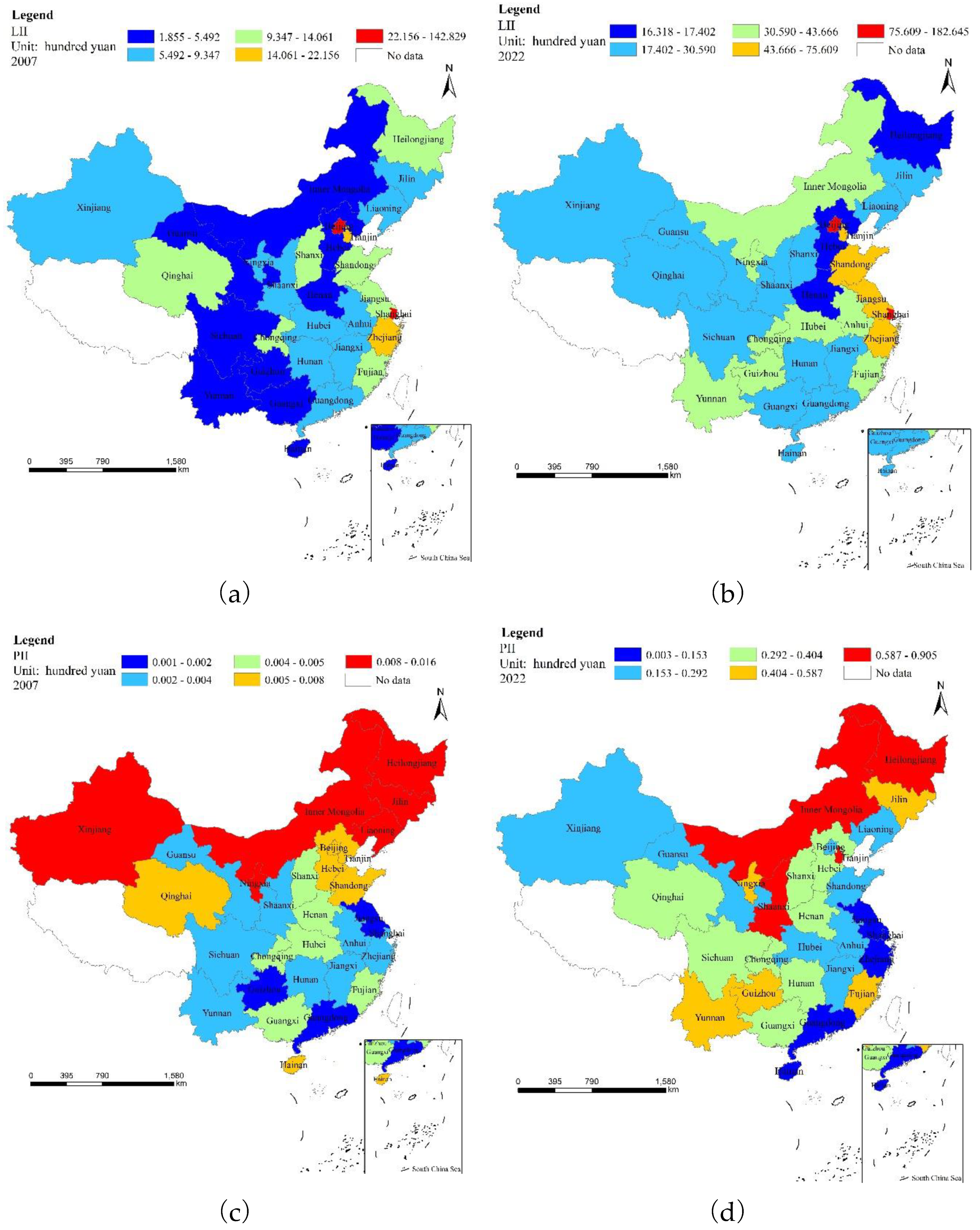
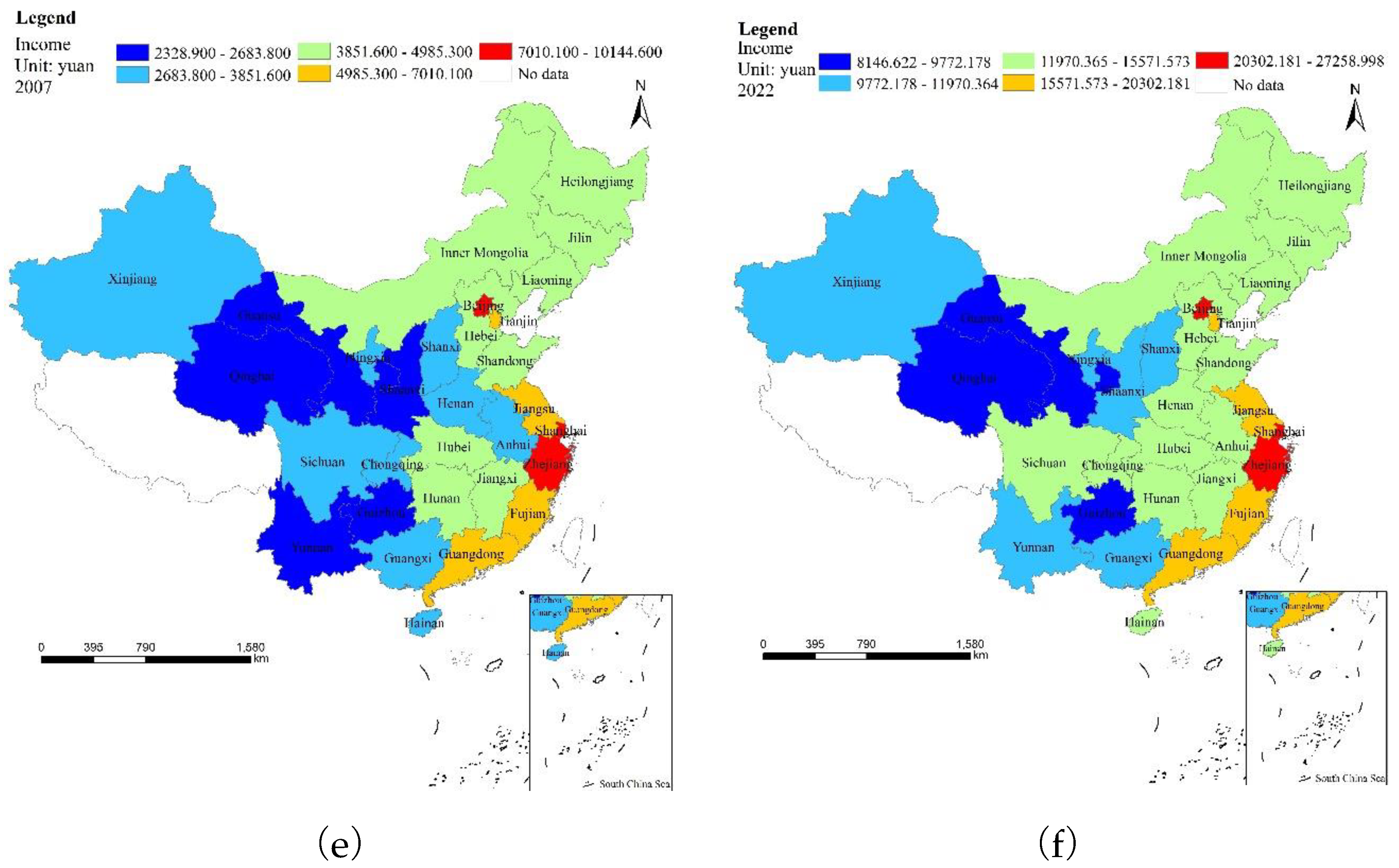
Figure 3.
Focus and standardized ellipse diagrams: (a) LII; (b) PII; (c) Villagers' income.
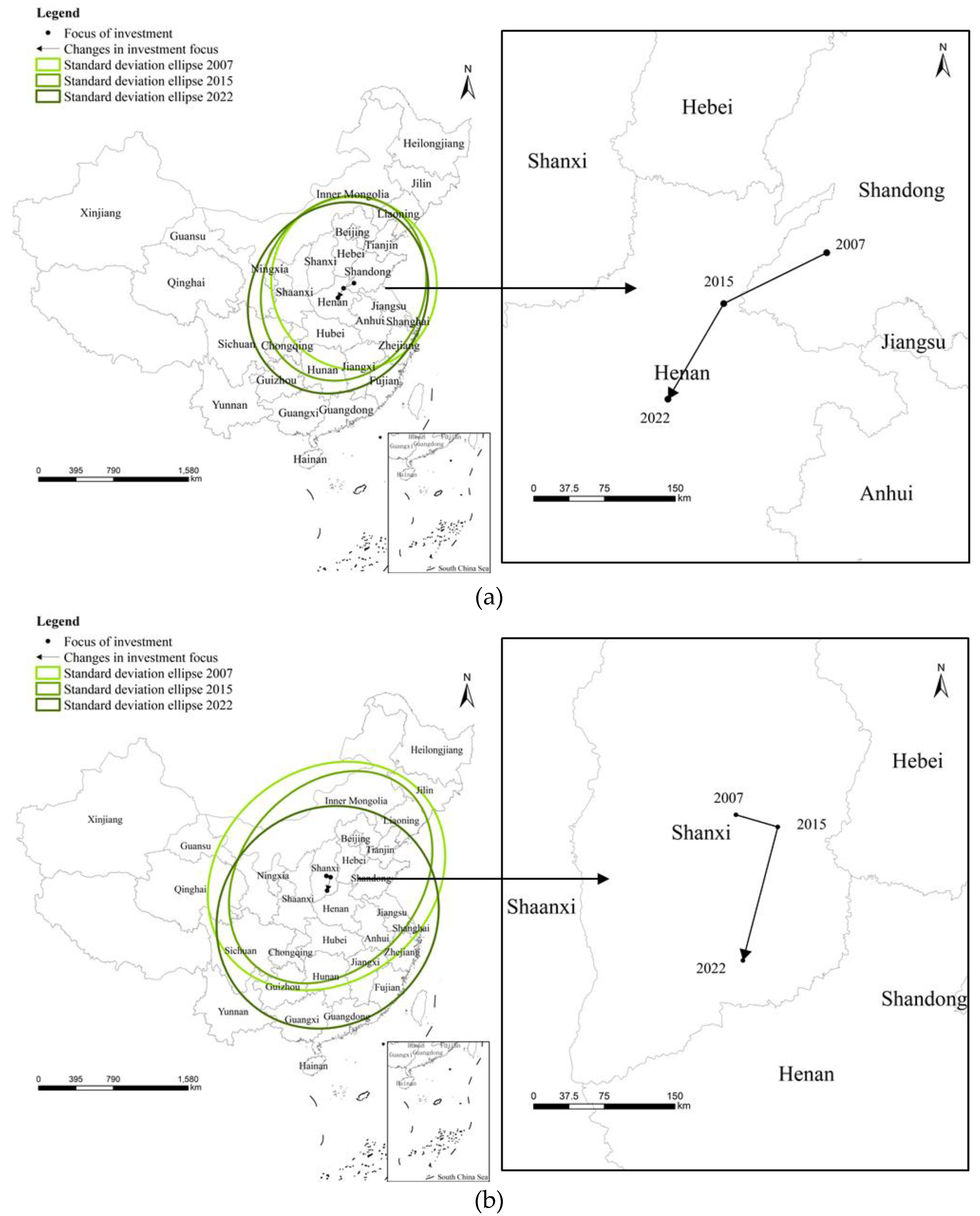
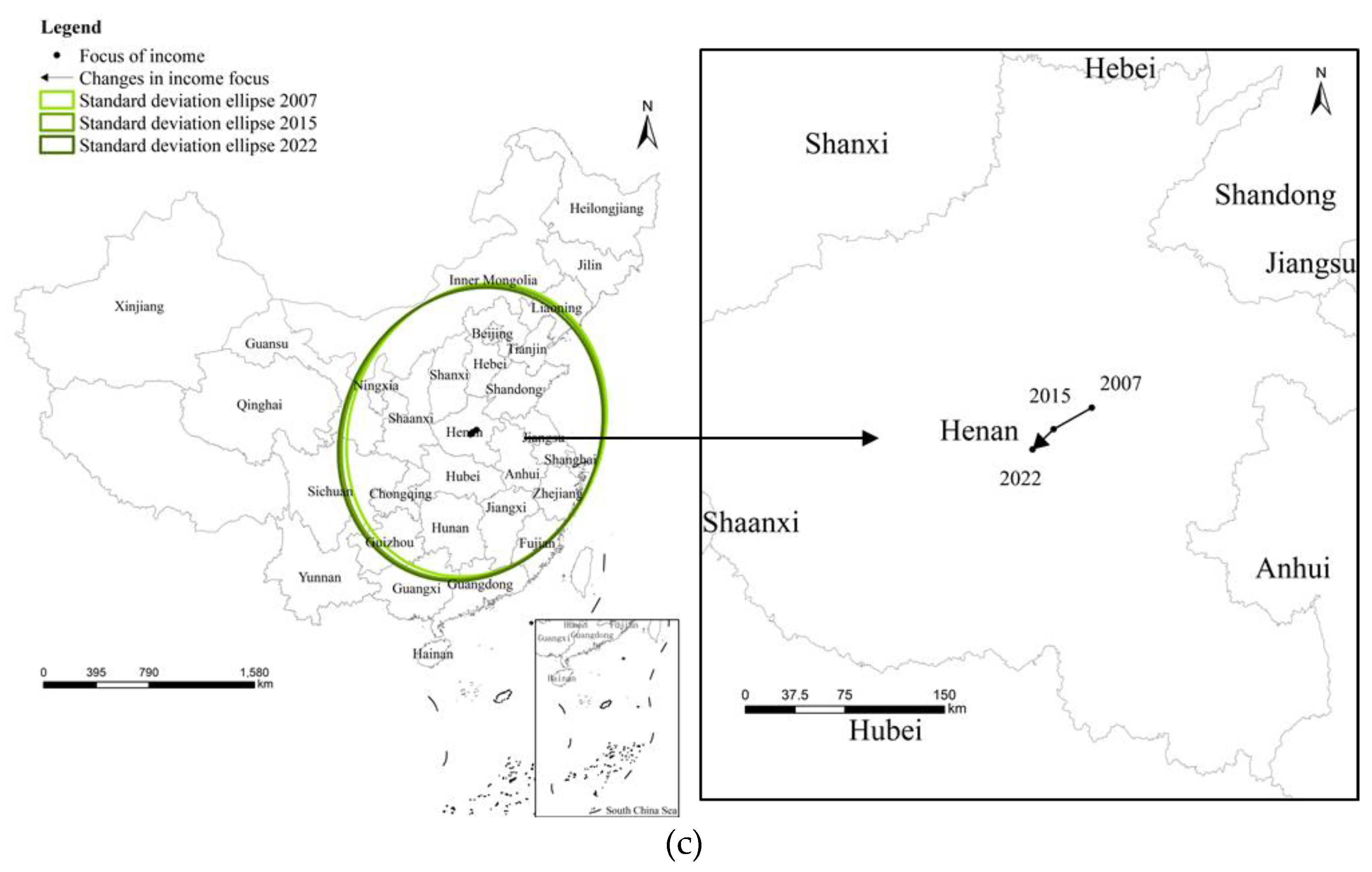

Table 1.
Variable definitions and descriptive statistics
| Variable name | Variable code | Meaning (unit) | Average value | Standard deviation | Minimum | Maximum | |
|---|---|---|---|---|---|---|---|
| Explained variables | Villagers' income | Per capita income of villagers (Ten thousand yuan) | 0.953 | 0.465 | 0.252 | 2.726 | |
| Villagers' wage income | Per capita wage income of villagers (Ten thousand yuan) | 0.418 | 0.337 | 0.039 | 1.779 | ||
| Villagers' non-wage income | Per capita non-wage income of villagers (Ten thousand yuan) | 0.535 | 0.205 | 0.167 | 1.124 | ||
| Explanatory variables | LII | Per capita LII (yuan) | 2523.900 | 3217.100 | 185.595 | 18807.080 | |
| PII | Per capita PII (yuan) | 1.560 | 1.354 | 0.113 | 8.573 | ||
| Control variables | job-related migration level | Number of migrant labors / aggregate labors (%) | 31.440 | 9.480 | 6.470 | 54.890 | |
| education level | Average years of education for rural population (year) | 7.779 | 0.650 | 5.878 | 10.118 | ||
| economic development level | Per capita GDP (Ten thousand yuan) | 3.608 | 2.039 | 0.538 | 11.932 | ||
| Urbanization level | Urbanization rate (%) | 58.182 | 13.039 | 29.110 | 89.600 | ||
| cultivated land endowment | Area of cultivated land managed by households / number of rural population (mu*) | 2.733 | 2.156 | 0.162 | 13.756 | ||
| Openness level | Total import and export volume / GDP(%) | 26.488 | 28.088 | 0.715 | 154.937 | ||
| Agricultural development level | Gross agricultural production / GDP(%) | 12.436 | 6.933 | 0.280 | 41.530 |
* 1 mu = 1/15 ha.
Table 2.
Results of standard deviation ellipse correlation parameters.
| Variable name | Year | Area (ten thousand km2) | Center point coordinates | Minor axis (km) | Major axis (km) | Flattening (unitless) |
Declination (°) |
|---|---|---|---|---|---|---|---|
| LII | 2007 | 249.956 | 115°54' E, 35°28' N | 871.350 | 913.152 | 0.046 | 170.098 |
| 2015 | 265.876 | 114° 37' E, 35°5' N | 849.830 | 995.910 | 0.147 | 22.455 | |
| 2022 | 299.508 | 113°52' E, 4°15'N | 913.901 | 1043.236 | 0.124 | 31.304 | |
| PII | 2007 | 467.753 | 112°24' E, 37°1' N | 1335.249 | 1115.135 | 0.165 | 51.183 |
| 2015 | 365.940 | 112°53' E, 36°52' N | 948.408 | 1228.257 | 0.228 | 40.147 | |
| 2022 | 431.681 | 112°21'E, 35°39' N | 1126.123 | 1220.251 | 0.077 | 44.408 | |
| Villagers' income | 2007 | 333.195 | 113°41' E, 33°44' N | 946.037 | 1121.150 | 0.156 | 22.577 |
| 2015 | 337.476 | 113°52'E, 33°51'N | 950.696 | 1129.989 | 0.159 | 24.812 | |
| 2022 | 339.595 | 114°12'E, 33°58'N | 960.270 | 1125.747 | 0.147 | 24.769 |
Table 3.
Results of the disparities between wage and non-wage income.
| Variable name | Villagers' income | Villagers' wage income | Villagers' non−wage income |
|---|---|---|---|
| 4e−05*** (8e−06) |
5e−05*** (6e−06) |
−8e−06 (5e−06) |
|
| 0.046*** (0.008) |
0.019*** (0.006) |
0.027*** (0.005) |
|
| 0.004** (0.002) |
0.003** (0.001) |
0.001 (0.001) |
|
| 0.127*** (0.026) |
0.071*** (0.019) |
0.056*** (0.010) |
|
| 0.110*** (0.010) |
0.055*** (0.008) |
0.055*** (0.007) |
|
| 0.013*** (0.002) |
0.003** (0.002) |
0.010*** (0.001) |
|
| −0.020** (0.009) |
−0.051*** (0.007) |
0.031*** (0.006) |
|
| −0.005*** (0.001) |
−0.004*** (0.001) |
−0.001 (0.001) |
|
| 0.005** (0.003) |
0.007*** (0.002) |
−0.002 (0.002) |
|
| _cons | −1.387*** (0.208) |
−0.607*** (0.154) |
−0.780*** (0.136) |
| F(9,411)=575.25*** | F(9,411)=245.27*** | F(9,411)=403.84*** |
Notes: ***/** indicate significance at the 1%/5% levels.
Table 4.
Results of the disparities between high-income and low-income.
| Variable name | Villagers' income | Villagers' wage income | Villagers' non−wage income |
|---|---|---|---|
| 10% quantile | |||
| 2e−05 (2e−05) |
4e−05** (2e−05) |
−9e−06 (1e−05) |
|
| 0.025 (0.022) |
0.012 (0.013) |
0.015 (0.013) |
|
| 25% quantile | |||
| 3e−05* (2e−05) |
4e−05*** (1e−05) |
−8e−06 (1e−05) |
|
| 0.033** (0.017) |
0.015 (0.009) |
0.020** (0.009) |
|
| 50% quantile | |||
| 4e−05*** (1e−05) |
5e−05*** (8e−06) |
−8e−06 (8e−06) |
|
| 0.046*** (0.012) |
0.019*** (0.006) |
0.027*** (0.007) |
|
| 75% quantile | |||
| 5e−05*** (1e−05) |
6e−05*** (1e−05) |
−7e−06 (1e−05) |
|
| 0.058*** (0.015) |
0.024*** (0.008) |
0.034*** (0.011) |
|
| 90% quantile | |||
| 7e−05*** (2e−05) |
6e−05*** (1e−05) |
−7e−06 (2e−05) |
|
| 0.068*** (0.022) |
0.026** (0.011) |
0.039*** (0.001) |
|
| Control variables are controlled. | |||
Notes: ***/**/* indicate significance at the 1%/5%/10% levels.
Table 5.
Correlation test results of spatial econometric model.
| Related tests | Value | P−value |
|---|---|---|
| LR test (SDM degenerates to SEM) | 376.85 | 0.000 |
| LR test (SDM degenerates to SAR) | 262.23 | 0.000 |
| AIC value of SDM | −1101.865 | - |
| AIC value of SEM | −743.017 | - |
| AIC value of SAR | −857.632 | - |
| Hausman test | 17.76 | 0.038 |
Table 6.
Spatial econometric analysis results.
| Variable name | Direct effect | Indirect effect | Total Effect |
|---|---|---|---|
| 4e−05*** (5e−06) |
6e−05*** (1e−05) |
1e−04*** (1e−05) |
|
| −0.011** (0.005) |
0.035*** (0.012) |
0.024* (0.013) |
|
| −0.004*** (0.001) |
0.017*** (0.003) |
0.013*** (0.003) |
|
| 0.011 (0.016) |
0.028 (0.037) |
0.039 (0.043) |
|
| 0.071*** (0.007) |
−0.042*** (0.016) |
0.029 (0.019) |
|
| −0.008*** (0.002) |
0.024*** (0.003) |
0.016*** (0.003) |
|
| −0.025*** (0.007) |
0.048*** (0.013) |
0.023 (0.016) |
|
| 0.001 (0.001) |
−0.002* (0.001) |
−0.002 (0.001) |
|
| 0.006*** (0.002) |
−0.020*** (0.004) |
−0.015*** (0.005) |
|
| rho | 0.289*** (0.049) |
Log−likelihood | 684.616 |
Notes: ***/**/* indicate significance at the 1%/5%/10% levels.
Table 7.
Heterogeneous impact of job-related migration and education.
| Variable name | Low level of job−related migration | High level of job−related migration | Low level of education | High level of education |
|---|---|---|---|---|
| 5e−05*** (1e−05) |
−2e−06 (1e−05) |
1e−05 (1e−05) |
4e−05*** (1e−05) |
|
| 0.037*** (0.011) |
0.041*** (0.008) |
0.084*** (0.010) |
0.032*** (0.011) |
|
| - | - | −0.002 (0.002) |
0.010*** (0.003) |
|
| 0.193*** (0.036) |
0.018 (0.026) |
- | - | |
| 0.096*** (0.014) |
0.135*** (0.013) |
0.084*** (0.013) |
0.136*** (0.014) |
|
| 0.026*** (0.003) |
0.015*** (0.002) |
0.020*** (0.002) |
0.020*** (0.004) |
|
| −0.029** (0.013) |
−0.002 (0.011) |
−0.018* (0.009) |
−0.145*** (0.040) |
|
| −0.006*** (0.001) |
2e−04 (0.001) |
0.003*** (0.001) |
−0.004*** (0.001) |
|
| 0.020*** (0.004) |
−0.001 (0.002) |
−0.001 (0.003) |
0.003 (0.004) |
|
| _cons | −2.668*** (0.331) |
−0.550*** (0.200) |
−0.599*** (0.110) |
−0.803*** (0.220) |
| F(8,188)=294.53*** | F(8,216)=703.06*** | F(8,216)=516.32*** | F(8,188)=310.17*** |
Notes: ***/**/* indicate significance at the 1%/5%/10% levels.
Disclaimer/Publisher’s Note: The statements, opinions and data contained in all publications are solely those of the individual author(s) and contributor(s) and not of MDPI and/or the editor(s). MDPI and/or the editor(s) disclaim responsibility for any injury to people or property resulting from any ideas, methods, instructions or products referred to in the content. |
© 2024 by the authors. Licensee MDPI, Basel, Switzerland. This article is an open access article distributed under the terms and conditions of the Creative Commons Attribution (CC BY) license (http://creativecommons.org/licenses/by/4.0/).
Copyright: This open access article is published under a Creative Commons CC BY 4.0 license, which permit the free download, distribution, and reuse, provided that the author and preprint are cited in any reuse.


