
Submitted:
18 November 2024
Posted:
19 November 2024
You are already at the latest version
Abstract
Accurate flow measurement is critical for hydraulic systems because it represents a crucial parameter in the control of fluid power systems and enables calculating hydraulic power when combined with pressure data, which is valuable for applications such as predictive maintenance. Existing flow sensors in fluid power systems typically operate invasively, disturbing the flow and providing inaccurate results, especially under transient conditions. A conventional method involves calculating the flow rate using the pressure difference along a pipe via the Hagen-Poiseuille law, which is limited to steady, laminar, incompressible flow. This paper presents a novel soft sensor with an analytical model for transient pipe flow based on two pressure signals, thus eliminating the need for an actual volumetric flow sensor. The soft sensor was derived in previous research and validated with a distributed parameter simulation. This work uses a constructed test rig to validate the soft sensor with real-world experiments. The results highlight the potential of the soft sensor to accurately and computationally efficiently measure transient pipe volumetric flow based on two pressure signals.
Keywords:
Soft sensor
; High-frequency compressible volumetric flow rate measurement
; Pressure-based sensor
; Pressure pulsation
; Cylinder coupling
1. Introduction
Volumetric flow measurement is critical to the longevity and performance of hydraulic systems. Accurate flow rate measurement is required for condition monitoring, predictive maintenance, and control engineering in mobile and stationary hydraulic systems. Knowing the volumetric flow rate in combination with pressure allows the calculation of hydraulic power, one of the most important parameters to characterize a fluid power system in terms of efficiency and potential losses. Furthermore, the volumetric flow rate represents a relevant fluid power system control variable.
Current volumetric flow sensors face two significant challenges. First, many must be physically installed inside the pipe, often using turbines or rotors that disrupt the flow and add complexity to the system. Second, these sensors contain mechanical parts with inertia that limit their effectiveness at high frequencies. For example, measuring pump pulsation becomes problematic because the pulsation frequency depends on the number of displacement units and the speed of the pump. In addition, pumps generate harmonic frequencies beyond the range of most state-of-the-art sensors. These limitations highlight the need for alternative methods of flow measurement. Ideally, a sensor would be minimal-invasive, capable of detecting transient flow conditions, and operate as a soft sensor using pressure signals commonly found in hydraulic systems.
The concept of deriving flow rates from pressure data has been introduced previously. Analytical methods for determining volumetric flow rates date back to the 19th century. One widely known method is the Hagen-Poiseuille law (HP) [1], which relates flow to the frictional pressure drop in a pipe. However, this law is limited to steady, laminar flow and does not account for high-frequency effects. The so-called Richardson effect [2] alters the velocity profile at higher frequencies. By incorporating a dynamic term into the Hagen-Poiseuille equation, it becomes possible to estimate transient flow rates. This paper presents an equation that led to developing a soft sensor for calculating transient flow rates based on pressure signals.
The following sections will cover the essential theoretical background and the development of the soft sensor. First, a brief overview of volumetric flow rate measurement techniques and models is provided in Section 2. Building on this foundation, the analytical model for the soft sensor is derived and examined in Section 2.3. The requirements for a suitable test rig are discussed, and the chosen concept is described. The soft sensor is then validated through multiple test cases presented in Section 2.5, followed by the results in Section 3. Finally, the paper concludes by discussing the findings and their implications.
2. Materials and Methods
2.1. Volumetric Flow Rate Measurement Methods
Accurate knowledge of volumetric flow is crucial to maintaining performance in fluid systems, leading to various sensors’ development. These sensors can generally be divided into two types: invasive and non-invasive.
Invasive sensors, such as positive displacement meters and turbine flow meters, determine volumetric flow by monitoring the movement of a given volume over time. However, due to the inertia of their components, they struggle to measure transient flows [3] accurately. A commonly used method in this category is to measure the pressure drop across a component designed to create flow resistance, such as an orifice [4]. The flow rate is derived from the following equation:
This equation is mainly independent of the fluid’s viscosity and is only slightly affected by temperature-induced variations in the density . The flow rate depends on factors such as the geometric parameter , the discharge coefficient , the fluid density , and the pressure difference . However, the intrusive installation of the orifice plate can significantly disrupt the flow pattern. A key challenge with differential pressure meters is their limited ability to handle unsteady flow, as the underlying Bernoulli principle assumes steady flow conditions. Research by Wiklund et al. [5] examining unsteady flow through differential pressure meters between and 10 Hz showed that these meters become unreliable for flows above 2 Hz.
Another invasive technique is using vortex flow meters, which base their measurements on the Kármán vortex street. Although this method results in a relatively low-pressure drop through the vortex body, its accuracy is compromised in laminar and low-turbulent flows due to its dependence on the Reynolds number (Re) [6]. Hot-wire anemometry (HWA) is another invasive technique used to measure flow velocity by detecting the cooling rate of a heated wire placed in the flow [7]. Despite its high sampling rate (up to 500 kHz [7]), HWA can only provide accurate point measurements and causes minimal flow disturbance. When multiple wires are required to capture a velocity profile, the mounting structure causes additional flow disturbance.
Non-invasive flow meters are the second category and have the advantage of not disturbing the flow or causing pressure drops. Electromagnetic flowmeters use Faraday’s law of induction, making them suitable for detecting transient flows without being invasive. However, the fluid must be conductive, with a minimum conductivity of [4], which is much higher than the conductivity of typical hydraulic oils such as HLP 46, which is around [8]. Ultrasonic flowmeters are another non-invasive option for measuring transient flows without significant system modifications. These sensors use two transducers mounted on the outside of the pipe to measure the time it takes for a signal to travel between them [9]. However, this method assumes symmetrical flow profiles, making it less accurate for turbulent flows that contain eddies.
An advanced, minimally invasive technique is particle image velocimetry (PIV), which uses laser-illuminated seeding particles in the fluid to map a two-dimensional velocity profile. The particle movements are recorded by cameras and processed to estimate flow velocity and, ultimately, volumetric flow rate [10]. However, PIV requires transparent piping, which is rarely feasible in industrial settings, and the introduction of seeding particles can contaminate the fluid. Another minimally invasive method is the Coriolis flowmeter, which passes the fluid through a vibrating bent tube, generating Coriolis forces proportional to the mass flow [4]. The measurement frequency is limited by the tube’s resonant frequency, with typical tubes limited to response times of 5 ms for a resonant frequency of 200 Hz. However, their vibrational frequencies can be much higher [11].
In summary, current volumetric flow sensors have several limitations. Many need to be more suitable for measuring transient flows due to slow response times, and those that offer faster response rates often impose requirements that cannot be met in typical industrial fluid systems.
2.2. Transient Flow Rate Models
Recent developments in transient flow measurement include significant contributions by Brereton et al. In one of their studies, they presented a method for treating arbitrary transients in laminar pipe flow, starting from an initial steady state, by relating the flow rate to the history of the pressure gradient without requiring assumptions about velocity profiles [12]. Later, in 2008, Brereton et al. introduced an alternative, indirect method that relates the flow rate to the history of the centerline velocity [13]. Sundstrom et al. [14] contributed by improving friction modeling, which significantly reduced errors in flow rate calculations in the pressure-time method commonly used for flow measurements in hydraulic systems. In 2019, Foucault et al. proposed a novel approach for time-resolved transient flow rate estimation based on differential pressure measurements. Their method exploited kinetic energy and relied on only two coefficients, effectively predicting laminar flow conditions in real time [15]. García et al. focused on unsteady turbulent pipe flow, validating their method through experiments involving the transient response of the velocity field following external perturbations, with a pressure step function as a test case [16]. Further work by García et al. in 2022 explored the transition from turbulent to laminar flow without an increase in bulk velocity, explaining the laminarization process through a newly developed mathematical model [17].
Urbanowicz et al. conducted a thorough review of analytical models for accelerated incompressible Newtonian fluid flow in pipes, comparing various methods based on imposed pressure gradients and flow rates while also analyzing their complexity and applicability to laminar and turbulent flows. Although these models perform well for laminar flows, they encounter challenges in accurately predicting turbulent flow behavior [18].
In 2023, Urbanowicz et al. advanced the modeling of laminar water hammer phenomena by developing an analytical solution validated by numerical simulations and experimental data [18]. Later that year, they proposed new analytical models for wall shear stress during water hammer events, extending the range of validity by incorporating quasi-steady and transient hydraulic resistance assumptions. These models simplified the mathematical representation and provided explicit analytical expressions further validated by numerical simulations [19]. Meanwhile, Bayle et al. investigated wave propagation models in water hammer scenarios. Their first study developed a rheology-based model for viscoelastic pipes validated with experimental data [20]. In a subsequent paper, they formulated a wave propagation model in the Laplace domain that could be applied to various boundary conditions in pipe systems [21].
Current advancements in transient flow measurement include methods for calculating flow rate based on pressure gradient history and centerline velocity, improved friction modeling for pressure-time accuracy, and real-time differential pressure estimation. Developments also cover unsteady turbulent flow analysis, laminarization modeling, analytical solutions for laminar water hammer, and wave propagation models for viscoelastic pipes, all validated by experimental data and simulations.
2.3. Analytical Soft Sensor Model for Flow Rate Calculation
The description and complete derivation of the analytical model of the soft sensor based on two pressure signals is provided in separate manuscripts [22,23] and is beyond the scope of this work. First, the equation for volumetric flow rate calculation under the assumption of an incompressible fluid was presented in the work of Brumand et al. [24]. In a second work by Brumand et al., [22], this equation was further investigated and expanded so that the compressible effects of the fluid are considered. The present work reiterates the main steps of the derivation to help the reader better understand. For more details regarding the derivation, the equations, and the variables used, please refer to the works of Brumand et al. mentioned above. The derivation of the system equations from the general Navier-Stokes equations is skipped in the present work, and the derivation begins from the so-called "two-dimensional viscous compressible model" as found in a literature review paper by Stecki [25]. The associated assumptions can also be found in Stecki’s work. Almondo [26] expanded on this model and proposed the solution for the volumetric flowrate at the outlet of the pipe as:
Inserting the propagation operator and the characteristic impedance yields:
In the following, the used variables are presented: is the modified Bessel function of the first kind of order n. is the normalized Laplace variable over the pipe radius R and the kinematic viscosity . is the dissipation number, with a being the speed of sound within the fluid and L the length of the pipe. Also, the hydraulic resistance of the pipe is defined as . The prefactors of the pressure functions are written as weighting functions as follows:
In the derivation it proved necessary to expand by a factor of to assure that the weighting functions have an inverse Laplace transformation. Therefore:
The weighting functions need to be inverse Laplace transformed (ILT). Then, the time solution of the volumetric flow rate is given in eq. 6. Note that the multiplication with the normalized Laplace variable of the pressure in eq. 5 corresponds to the derivative of the pressure with respect to the normalized time in the time domain in eq. 6, therefore: . Also note that a multiplication in the Laplace domain of two functions, here and equals a convolution integral in the time domain. [27]
The needed inverse Laplace transforms of the weighting functions are given by the sum of their residues around the poles of the functions at [28]:
where N is a natural number for the upper bound of the sum. For the ILT, knowing the position of the poles is necessary. First, the poles for the incompressible case are evaluated. Incompressible fluids have a speed of sound a tending to ∞, which leads to a dissipation number tending to zero: . For the incompressible case, using and , the weighting functions become:
Firstly, it can be observed that the function has a double pole at . Additionally, the residues at the remaining simple poles of the weighting function stem from the Bessel function. Bessel functions have an infinite amount of increasing simple poles that can be expressed as:
The residue of the double pole at can be calculated by use of eq. 10 [28]:
Left are the residues at the remaining simple poles of the weighting function at . The first eight poles, depending on the Bessel function, lie at:
With the double pole at in eq. 10, the ILT of the incompressible weighting function further depends only on simple poles to which the residue can be calculated more directly by [28]:
Inserting the numerator and denominator of the incompressible weighting function into eq. 12 yields the inverse Laplace transformed function of as:
Inserting the poles into the sum gives:
The poles for the case of (case of a compressible fluid) are the same as for (case of an incompressible fluid) in addition to the poles caused by the hyperbolic terms. For the ILT, knowledge about the position of the poles and the order is necessary. To gain information about the order of the poles, an approximation is used for the sinh function that keeps the characteristics of the poles [29]:
The poles of both weighting functions are at , and by using eq. 15:
Rearranging for , we obtain:
This equation was solved for the poles using the software Maple [30] for various dissipation numbers. The dissipation numbers range from to , with 100 samples per order of magnitude. For each sampled dissipation number, the first 20 poles were computed. Poles that are bigger than that have a negligible effect on the flow rate. This matrix functions as a lookup table for which poles to use during the computation of the volumetric flow rate. Rounding the dissipation number to the nearest sampled dissipation number did not have a visible impact on the result.
With knowledge of the poles, the residues of the time domain solution for each dissipation number can be calculated using eq. 18:
The computation of the residues was automated using the Maple software. Now the weighting function in the time domain () is given by:
An exemplary weighting function is presented in the following as a clarification for the reader. Assuming , and using eq. 17, the first five poles are located at:
- .
For this exemplary dissipation number, the compressible effects are considered by the following weighting function, consisting of the residues caused by the poles of the sinh function:
Together with the incompressible weighting function (eq. 14) caused by the incompressible poles, the whole weighting function is given by:
Note that depends on the dissipation number . For a treatise of the resulting convolution integral for calculating the volumetric flow rate (eq. 6), please refer to the manuscript by Brumand et al. [22].
2.4. Test Rig
A suitable test rig concept had to be developed to validate the derived system equations for the soft sensor. The main task of the test rig is to provide a known transient flow rate through a hydraulically smooth, straight pipe. This measuring pipe must fulfill the assumptions made in the system equations. Furthermore, measuring pressure signals at at least two positions in the measuring line must be possible. The pressure difference for the system equation is formed from these measurement signals. The calculated volumetric flow rate is then compared with the volumetric flow rate provided by the test rig. The test rig should be able to generate different flow conditions in the laminar and turbulent Reynolds number range. The behavior of hydraulic pumps was considered to estimate the achievable flow conditions. These generally provide a non-constant volumetric flow rate Q, with the degree of non-uniformity indicating the size of the pulsation that occurs. Depending on the pump type of the hydraulic pump, undesirable degrees of non-uniformity of up to = may occur [31]. The frequency of these pulsations can be estimated further for pumps that operate according to the positive displacement principle and have an odd number of pistons [32].
There are multiple approaches for generating specific pulsations within fluid power systems. One widely used approach involves placing a valve directly into the fluid stream and controlling the flow rate by adjusting the valve [33]. In this method, the oscillation frequency and amplitude are primarily governed by the valve’s dimensions and the system’s natural resonance frequency. Another technique employs a side-discharge valve [34], which offers a key advantage because it diverts only a portion of the flow through the valve. This enables the use of a smaller, quicker valve. Despite the differences, both methods focus primarily on creating and analyzing pressure waves within the system. Thus, more than these methods are needed to measure the unsteady flow rates with high precision.
Generating pulsation via a hydraulic cylinder’s movement and geometric displacement is more promising. The displaced volumetric flow rate can be approximately calculated via the kinematics of the cylinder using , whereby the movement can be generated in different ways. For example, a cylinder used as a displacer could be activated via a thrust crank or by coupling with another cylinder. When calculating the reference volumetric flow rate in this way, it is essential to note that compressibility effects and effects caused by the propagation of generated pressure waves are not considered. Therefore, measures must be implemented to minimize these effects, as calculating the transient volumetric flow rate would otherwise be highly susceptible to errors. The error resulting from the compressibility effects can be reduced by operating at higher pressures associated with higher and more steady bulk modulus K. Further errors occurred due to wave reflection in the pipe. This is because pressure waves are reflected when the characteristic impedance changes, which could significantly change the volumetric flow within the measurement pipe. These changes occur, for example, at points of installations in the pipe or when the pipe cross-section changes [35]. This results in the requirement to reduce cross-sectional changes to a minimum and to terminate the measurement pipe with a low-reflection line terminator (LRLT).
A LRLT generally consists of an orifice, an adjustment mechanism for variable adjustment of the orifice cross-section, and a volume behind it. By adjusting the orifice’s cross-section, the impedance of the orifice can be matched to the pipe’s characteristic impedance, and thereby the LRLT imitates an infinitely long pipe. The pressure wave is not reflected and propagates in the volume of the low-reflection pipe termination. The structure of such a low-reflection line termination is illustrated in Figure 1. The effect of the adjustment on the measured pressure waves in a pipe is shown in Figure 2. Suppose the orifice cross-section is not adjusted appropriately, and pressure transducers are installed at three locations of a connected measurement pipe. In that case, incoming pressure waves are reflected at the low-reflection line termination, and the pressure histories show a noticeably smaller pressure amplitude and a phase shift (correct figure) compared to the correctly adjusted LRLT (left figure). As in this example, a harmonic volumetric flow rate was induced. The LRLT can not be adjusted by viewing the measured pressure histories, and instead, an adjustment based on a calculated pressure drop across the orifice was done [35].
Based on the stated requirements and the challenges associated with providing a reference transient volumetric flow rate, a test rig concept was developed and validated in the work of Brumand-Poor et al. [24]. The hydraulic circuit of this test rig is displayed in Figure 3.
The core component of the test rig is the measurement pipe with a length of m, which includes three designated locations for pressure measurements. The distances between the first and second pressure transducers, PT1 and PT2, and between PT2 and PT3, are l12 m and l23 m, respectively. The measurement pipe is terminated on both sides by LRLT1,2 to prevent the reflections of pressure waves, with each LRLT positioned lLT= lTL m from the nearest T-fitting. The adjustable orifice O1 allows for adjusting the pressure inside the measurement pipe to reduce compressibility effects. The LRLT1 is also connected to the steady flow supply, which includes a hydraulic pump (P1), a pressure relief valve (PRV1), and a volumetric flow rate sensor (VF1). The measurement pipe is also connected to the dynamic flow source, comprising a double-rod cylinder (DRC) that drives two single-rod cylinders (SRC1,2) to generate the dynamic volumetric flow rate. The T-fittings connecting the measurement pipe to the dynamic flow source are distanced lT1 m from PT1 and l3T m from PT3, ensuring sufficient inlet and outlet zones. The double-rod cylinder is actuated by a control valve CV1 to precisely control the amplitude and shape of the provided flow, allowing varying operating points. The velocity of the piston movement is measured with a position sensor connected to one of the rods. Additionally, the dynamic flow source is equipped with a hydraulic pump P2, a pressure relief valve PRV4, and a switching valve SV3. The switching valves allow for pre-pressurization of the single rod cylinders to balance the force of the pressure in the measurement pipe and thus reduce stress on the connection of the cylinders. Further, the coupling of the single-rod cylinders ensures that the fluid volume within the measurement pipe remains unchanged, as the suction action of the other pulls in the volume displaced by one cylinder. This is important as the LRLT adjustment depends on the volumetric flow rate. Thus, the orifice of both of the LRLT is adjusted based on the mean volumetric flow rate provided by the pump P1 as shown in eq. (24). Any deviations in the volumetric flow rate through the orifice from lead to a change in characteristic impedance. This introduces an error in the volumetric flow rate calculation, which increases with increasing frequencies. [24] Also, the switching vales SV1,2 enable the operation of the test bench in either an oscillating or pulsating mode. At the same time, pulsating means the overlap of the mean volumetric flow rate with the dynamic . For validating the soft sensor, the volumetric flow rate computed from pressure measurements is compared with the test rig’s flow rate calculated as .
As depicted in Figure 4, the realization of the test bench concept is shown. The image highlights critical components: the LRLT1,2, circled in red, connected to both ends of the measurement pipe (circled in orange). Additionally, the coupled cylinders (circled in blue) are crucial in generating the dynamic volumetric flow rate, as they are responsible for the oscillating fluid movement. One of the critical challenges in this setup is ensuring the pressure transducers are integrated to provide highly accurate pressure measurements, as these are crucial for the soft sensor’s calculation of the volumetric flow rate. To achieve this, a custom cutting ring fitting was developed. This specialized fitting connects two pipe segments without altering the internal diameter from the measurement pipe to the fitting. It allows the installation of up to three pressure transducers at a single point along the pipe. A cross-sectional view of the fitting is provided in Figure 5.
2.5. Test Cases
Different flow scenarios were tested to validate the novel equation. First, a steady volumetric flow rate was chosen. Then, the degree of non-uniformity of the flow rate and the frequency for the superimposed sine wave was determined. A mean system pressure of 100 bar guarantees that the compression effect is significantly reduced. The chosen combinations of volumetric flow rates and pressure are suitable so that the pump can deliver a steady laminar flow.

Table 1.
Pressure conditions set for each test case.
| Test Case | System Pressure [bar] |
Mean Volumetric Flow Rate [l/min] |
Degree of Non-uniformity [-] |
Frequency f [Hz] |
|---|---|---|---|---|
| Sine (Figure 6, Figure 7 and Figure 8) | 100 | 40 | , , | 5 |
| Sine (Figure 9, Figure 10 and Figure 11) | 100 | 40 | , , | 10 |
| Sine (Figure 12, Figure 13 and Figure 14) | 100 | 50 | , , | 15 |
3. Results
This section shows the agreement between the measured flow rate, composed of the steady flow rate by the pump and the calculated dynamic flow rates from the movement of the cylinders, and the flow rate calculated by the novel equations using two pressure sensors in the pipe. The presented flow rates are obtained by PT1 and PT2, which have the smallest distance regarding the three pressure transducers.
The raw measured signals were filtered using a first-order Butterworth filter [36] with a cutoff frequency slightly above the analyzed frequency. For a good comparison, both signals were aligned so that the peaks of the sine waves align. This phase offset was caused by the compression effects of the oil as well as the filtering process. The performance of the soft sensor characterized by the mean error and the standard deviation of the volumetric flow rate computed by the test rig and the soft sensor is provided in Table 2.
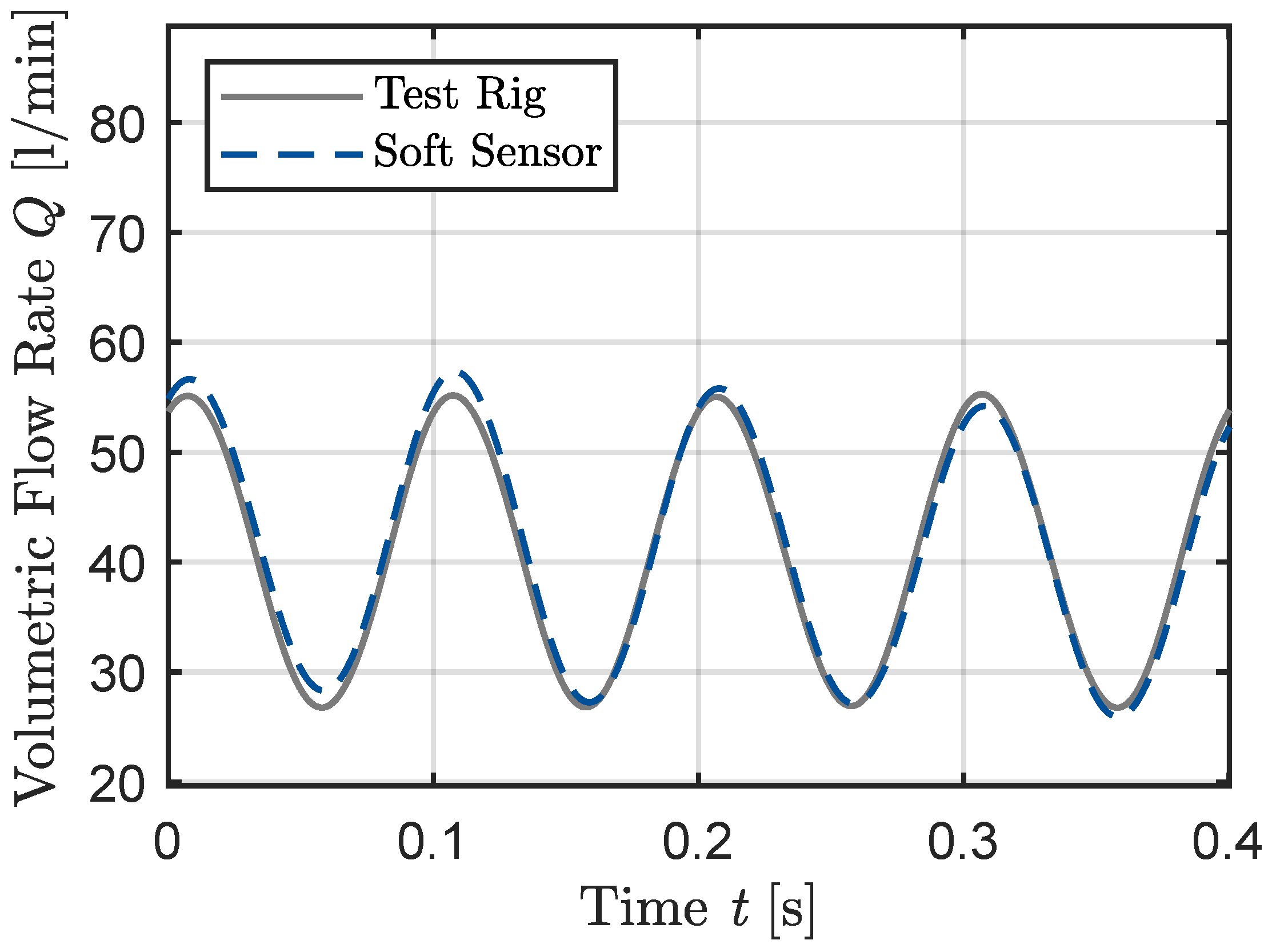
For 5 Hz, both signals show good alignment, as can be seen in Figure 6, Figure 7 and Figure 8. The mean errors were: , and , with standard deviations of , and .
Figure 6.
Measurement of sine wave with a frequency of Hz, a degree of non-uniformity of and a steady flow rate of l/min.
Figure 6.
Measurement of sine wave with a frequency of Hz, a degree of non-uniformity of and a steady flow rate of l/min.
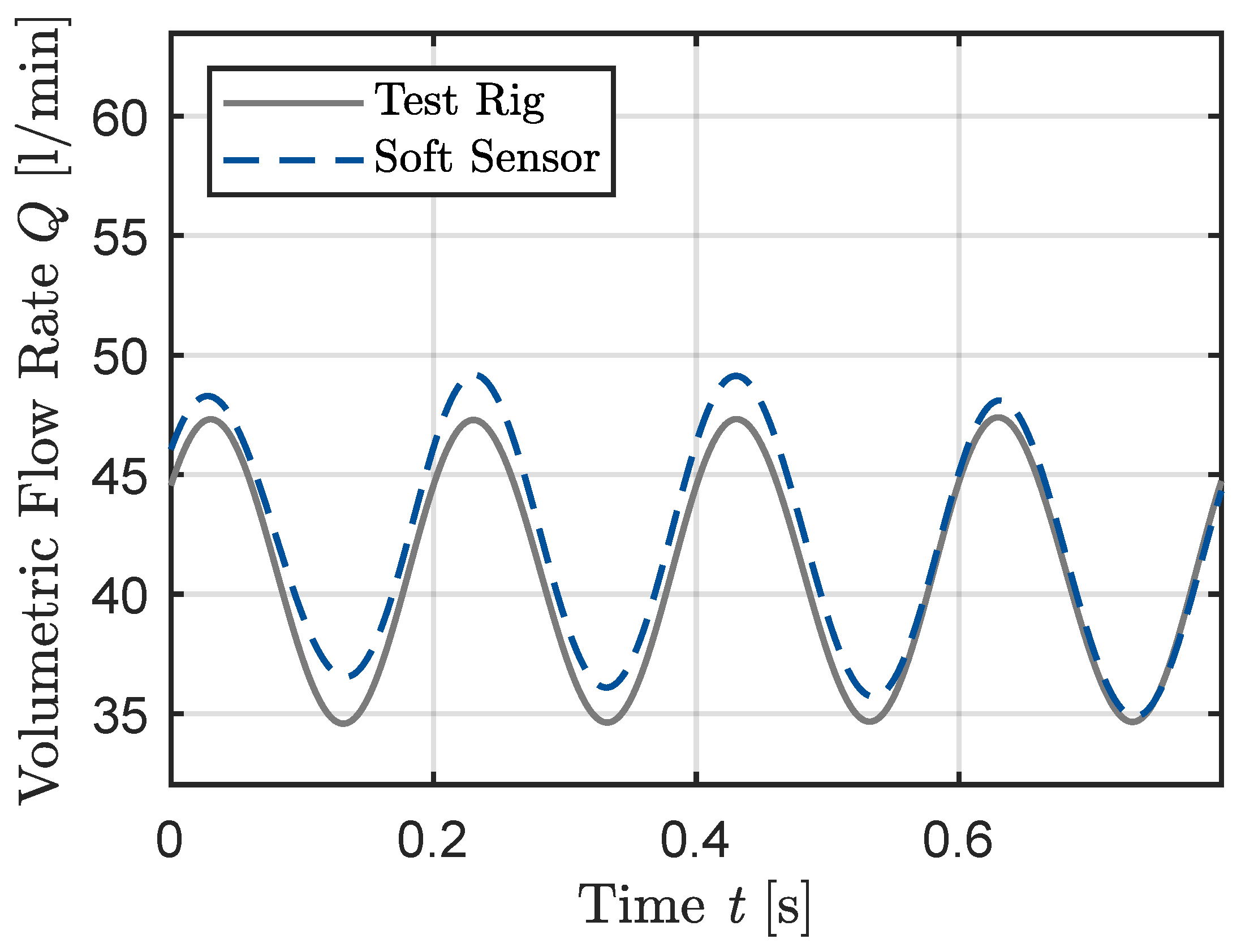
Figure 7.
Measurement of sine wave with a frequency of Hz, a degree of non-uniformity of and a steady flow rate of l/min.
Figure 7.
Measurement of sine wave with a frequency of Hz, a degree of non-uniformity of and a steady flow rate of l/min.
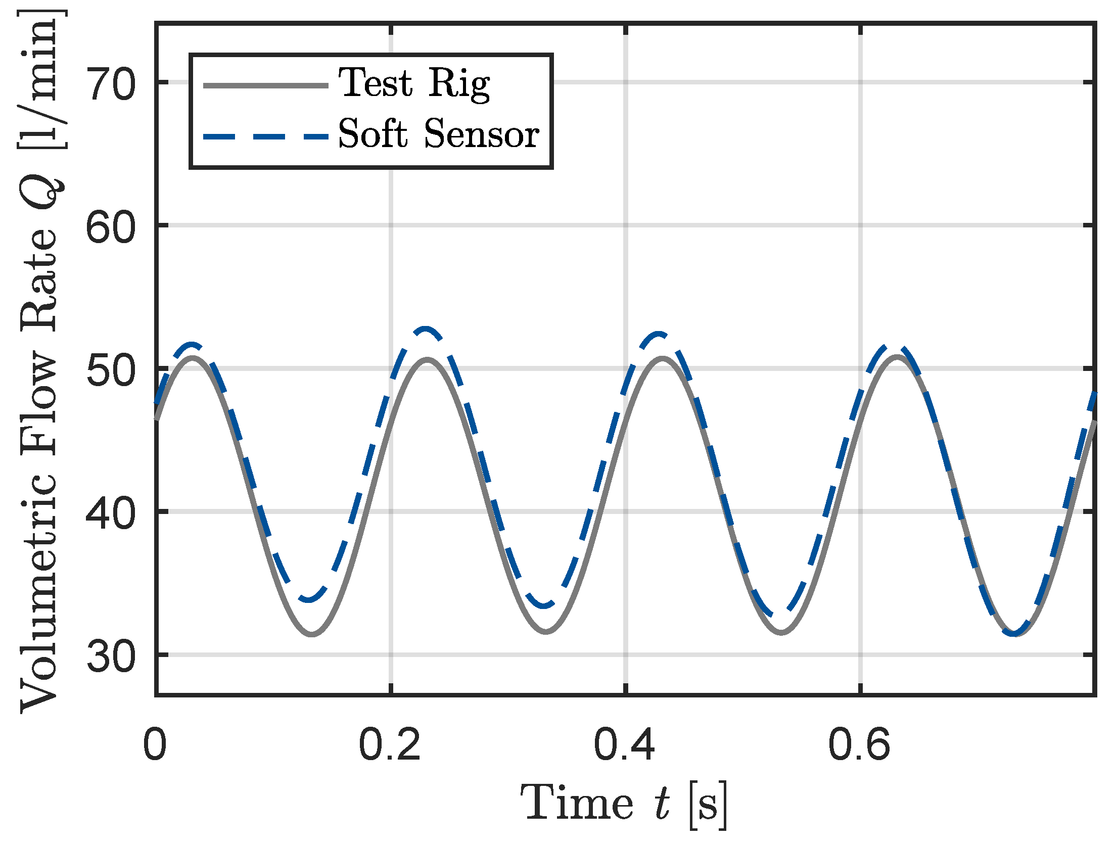
Figure 8.
Measurement of sine wave with a frequency of Hz, a degree of non-uniformity of and a steady flow rate of l/min.
Figure 8.
Measurement of sine wave with a frequency of Hz, a degree of non-uniformity of and a steady flow rate of l/min.
In the case of a sine wave with 10 Hz, good agreement was achieved between the novel equation and the measured flow rate as shown in Figure 9, Figure 10 and Figure 11. The mean errors were: , and , with standard deviations of , and .
Figure 9.
Measurement of sine wave with a frequency of Hz, a degree of non-uniformity of and a steady flow rate of l/min.
Figure 9.
Measurement of sine wave with a frequency of Hz, a degree of non-uniformity of and a steady flow rate of l/min.
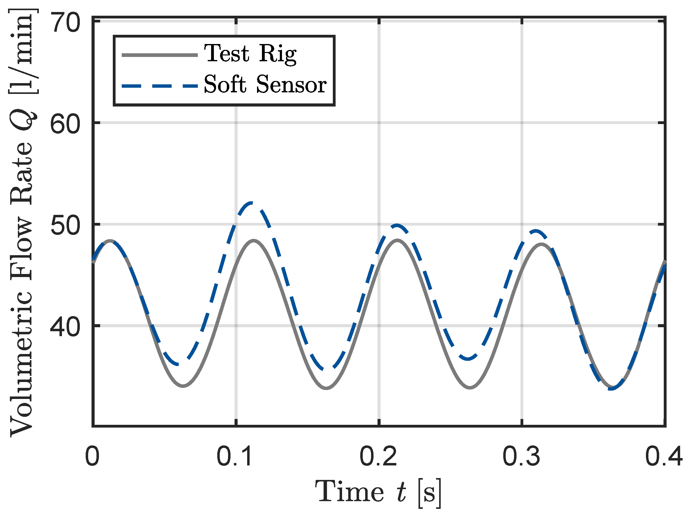
Figure 10.
Measurement of sine wave with a frequency of Hz, a degree of non-uniformity of and a steady flow rate of l/min.
Figure 10.
Measurement of sine wave with a frequency of Hz, a degree of non-uniformity of and a steady flow rate of l/min.
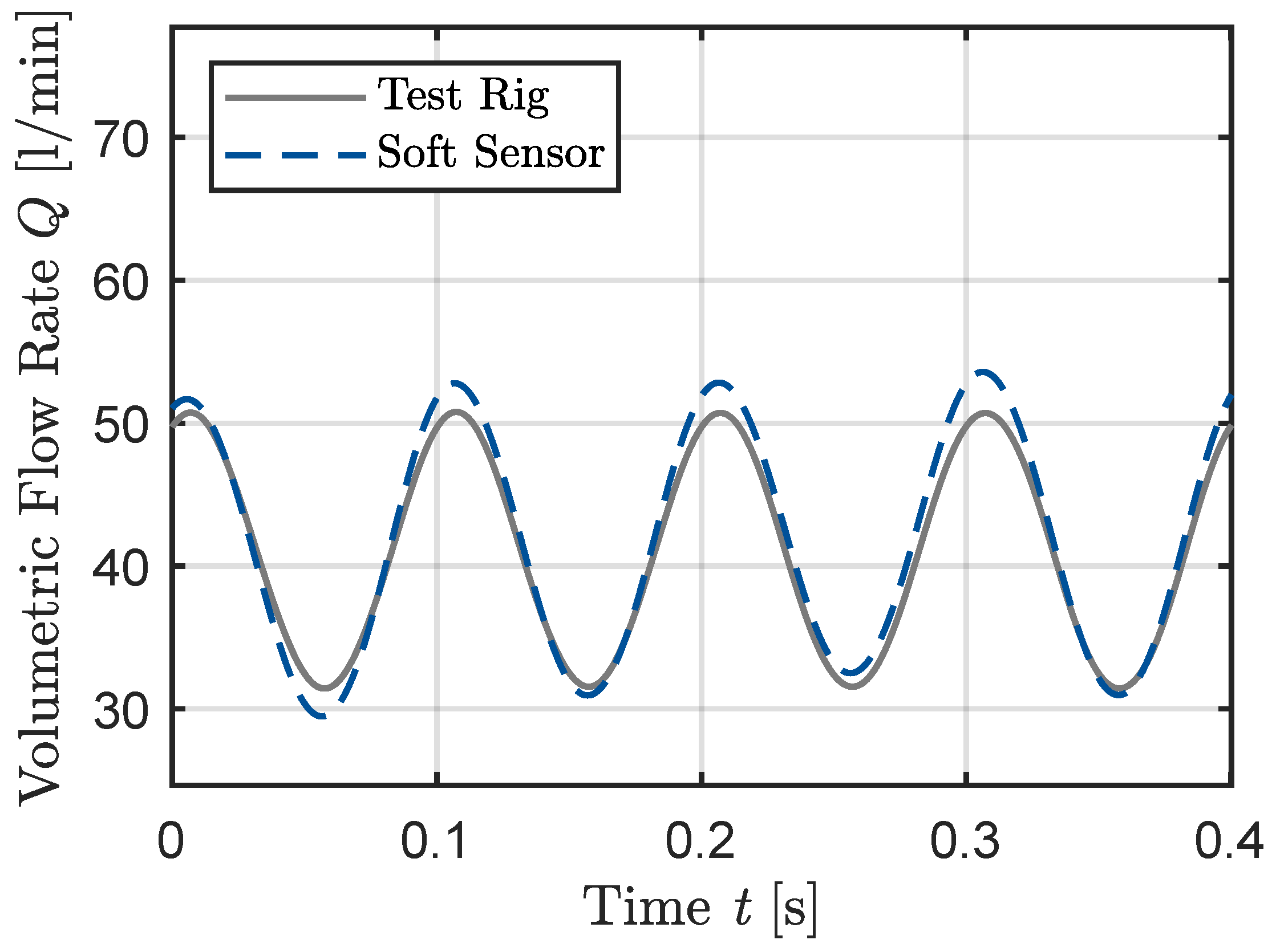
Figure 11.
Measurement of sine wave with a frequency of Hz, a degree of non-uniformity of and a steady flow rate of l/min.
Figure 11.
Measurement of sine wave with a frequency of Hz, a degree of non-uniformity of and a steady flow rate of l/min.
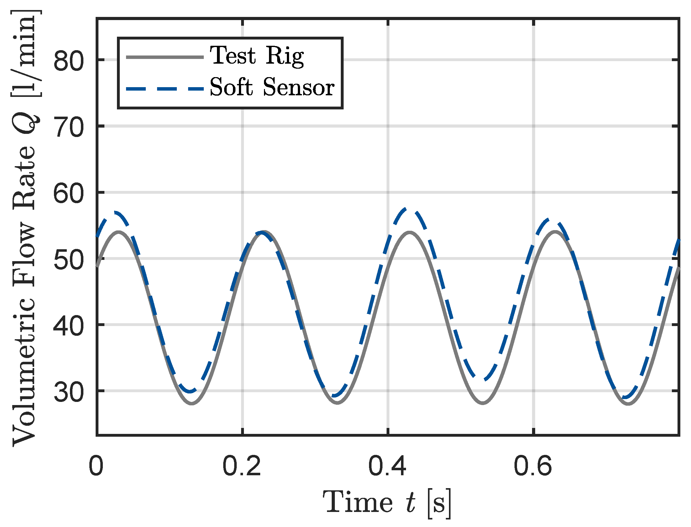
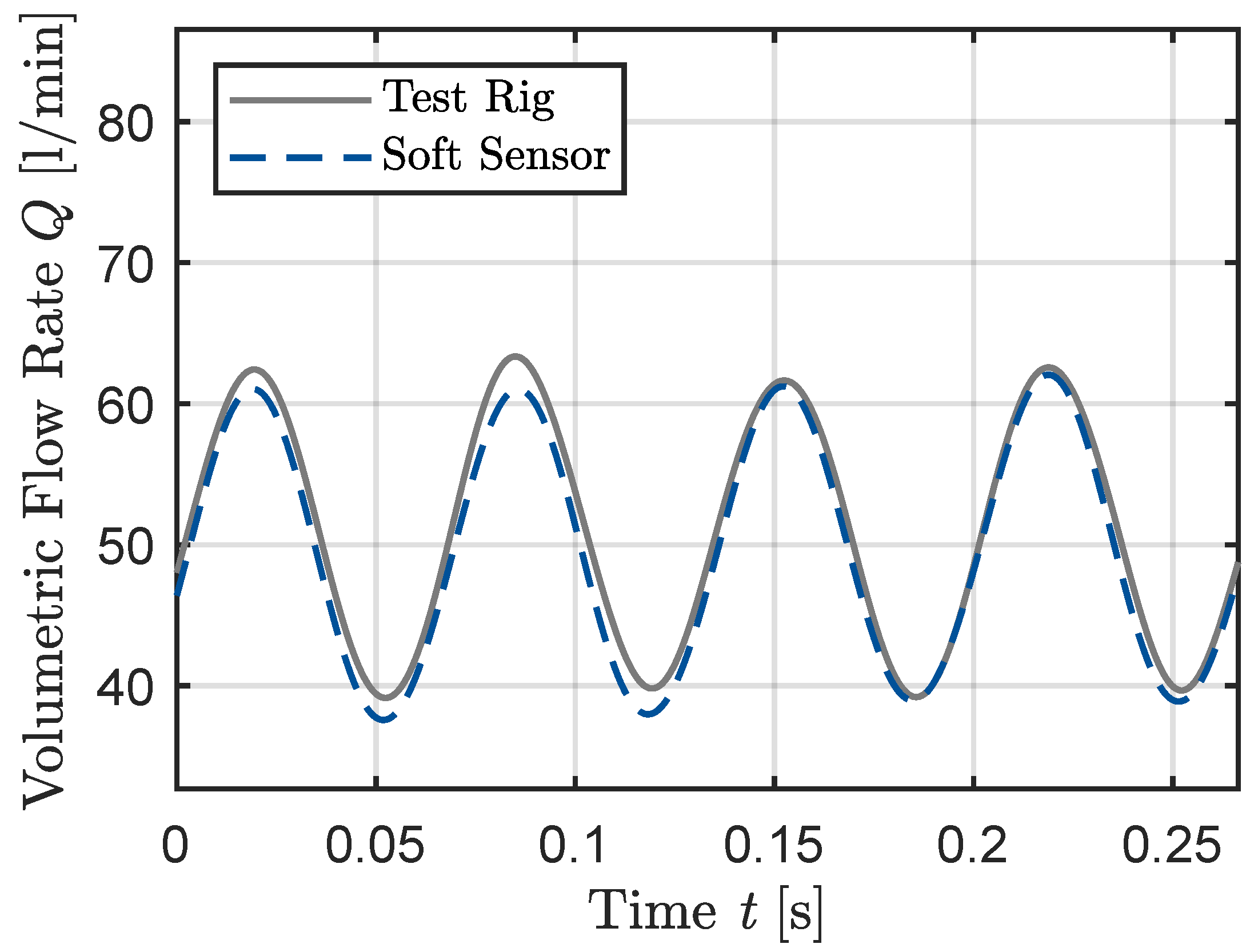
Lastly, the case of a sine wave with Hz showed the least agreement, but the novel equation still managed to represent the system’s behaviour. The mean errors were: , and , with standard deviations of , and .
Figure 12.
Measurement of sine wave with a frequency of Hz, a degree of non-uniformity of and a steady flow rate of l/min.
Figure 12.
Measurement of sine wave with a frequency of Hz, a degree of non-uniformity of and a steady flow rate of l/min.
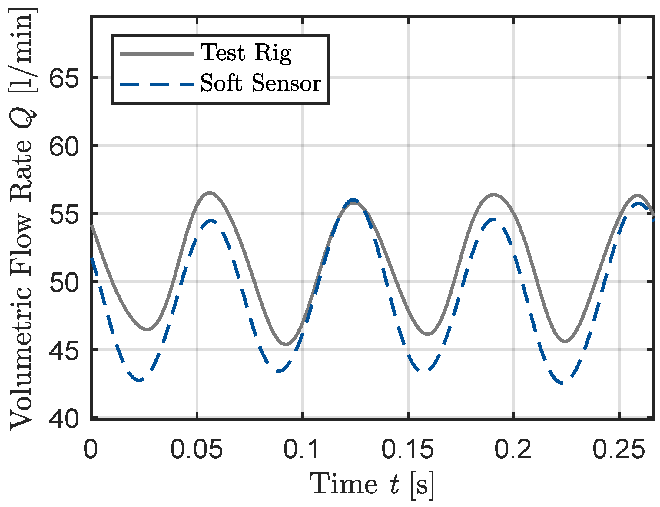
Figure 13.
Measurement of sine wave with a frequency of Hz, a degree of non-uniformity of and a steady flow rate of l/min.
Figure 13.
Measurement of sine wave with a frequency of Hz, a degree of non-uniformity of and a steady flow rate of l/min.

Figure 14.
Measurement of sine wave with a frequency of Hz, a degree of non-uniformity of and a steady flow rate of l/min.
Figure 14.
Measurement of sine wave with a frequency of Hz, a degree of non-uniformity of and a steady flow rate of l/min.
In all cases analyzed, the mean error and standard deviation were below , which shows that the novel equation agrees well with reality.
4. Discussion
The presented results show the promising ability of the soft sensor to measure transient volumetric flow rates accurately. The developed sensor utilizes the signals of two pressure transducers in a pipe to compute the transient flow rate efficiently and accurately. The computation is real-time due to the analytical model of the soft sensor. The computed volumetric flow rate matches well with the reference flow rate provided by the test rig. Several test cases are created by the coupled cylinder and pump, which are investigated and compared to the soft sensor. Different sine waves with varying frequencies and degrees of non-uniformity are investigated.
The soft sensor captures frequencies up to 15 Hz and degrees of non-uniformity up to with reasonable accuracy. Notably, the sensor matches the amplitude and phase of the created flow rate. The mean error in all measurements is below , and the overall mean error considering all measurements at once is around . The standard deviation of the error is also below , underlining the good performance of the soft sensor. Furthermore, the smallest distance between the pressure transducers, l12 m, was used to obtain the volumetric flow rate, underlining the high accuracy and feasibility of the soft sensor.
5. Conclusions
This paper demonstrates the ability of an analytical soft sensor to determine transient volumetric flow rates based on two pressure signals in a pipe. It begins with an introduction to currently established volumetric flow rate measurements and transient flow rate models. It then describes the soft sensor and presents the test rig constructed and the test cases studied for validation.
The analytical soft sensor accurately and efficiently measures the transient volumetric flow rate provided by the test rig for the nine different test cases. The sensor agrees well with the volumetric flow rate for transient flows up to 15 Hz and a degree of non-uniformity up to .
The results of this research represent a significant advancement in soft sensors for transient flow rate measurement. This work presents a novel method for obtaining accurate and efficient pipe volumetric flow rates using two pressure transducers. The soft sensor is based on an analytical model that accurately and computationally efficiently determines the volumetric flow rate. The results underscore the potential of the soft sensor for use in various industrial applications, such as condition monitoring and control, where real-time and accurate computation of critical system parameters is essential. In addition, the sensor’s ability to track pressure and flow rate enables the calculation of hydraulic power, which can be used for predictive maintenance and provides deeper insight into system performance. Compared to existing sensors, the soft sensor is minimal-invasive and can be applied only with the information from the pressure signals. Compared to numerical simulations, the soft sensor can obtain a real-time solution, which is usually impossible due to numerical computation.
Author Contributions
Conceptualization, Faras Brumand-Poor, Tim Kotte, Marwin Schüpfer, Felix Figge and Katharina Schmitz; Data curation, Faras Brumand-Poor, Tim Kotte and Marwin Schüpfer; Formal analysis, Faras Brumand-Poor, Tim Kotte, Marwin Schüpfer and Felix Figge; Funding acquisition, Faras Brumand-Poor and Katharina Schmitz; Investigation, Faras Brumand-Poor, Tim Kotte and Marwin Schüpfer; Methodology, Faras Brumand-Poor, Tim Kotte and Marwin Schüpfer; Project administration, Faras Brumand-Poor and Katharina Schmitz; Resources, Faras Brumand-Poor, Tim Kotte, Marwin Schüpfer and Katharina Schmitz; Software, Faras Brumand-Poor, Tim Kotte and Marwin Schüpfer; Supervision, Faras Brumand-Poor; Validation, Faras Brumand-Poor, Tim Kotte and Marwin Schüpfer; Visualization, Faras Brumand-Poor, Tim Kotte and Marwin Schüpfer; Writing – original draft, Faras Brumand-Poor, Tim Kotte and Marwin Schüpfer; Writing – review & editing, Faras Brumand-Poor, Tim Kotte, Marwin Schüpfer, Felix Figge and Katharina Schmitz. All authors have read and agreed to the published version of the manuscript.
Funding
The IGF research project 21475 N / 1 of the research association Forschungskuratorium Maschinenbau e. V. (FKM), Lyoner Straße 18, 60528 Frankfurt am Main was supported by the budget of the Federal Ministry of Economic Affairs and Climate Action through the AiF within the scope of a program to support industrial community research and development (IGF) based on a decision of the German Bundestag.
Data Availability Statement
The datasets presented in this article are not readily available because the data are part of an ongoing study.
Conflicts of Interest
The authors declare no conflicts of interest.
Abbreviations
The following abbreviations are used in this manuscript:
| BV | Ball Valve |
| CV | Control Valve |
| DRC | Double-rod Cylinder |
| HD | Hydraulic Damper |
| HP | Hagen-Poiseuille |
| HWA | Hot-wire Anemometry |
| ILT | Inverse Laplace transformation |
| LRLT | Low-reflection line terminator |
| O | Adjustable Orifice |
| P | Hydraulic Pump |
| PIV | Particle Image Velocimetry |
| PT | Pressure Transducer |
| Re | Reynolds number |
| SRC | Single-rod Cylinder |
| SV | Switching Valve |
| VF | Volumetric Flow Rate Sensor |
Nomenclature
| Symbol | Definition | Unit |
| * | Denotation of a Variable in the Laplace Domain | [m2/s] |
| a | Speed of Sound | [m/s] |
| A | Cross-section of the Cylinder | [m2] |
| Geometric Parameter | [m2] | |
| Cross-section of the Pipe | [m2] | |
| Dissipation Number | [-] | |
| f | Frequency | [Hz] |
| Propagation Operator | [-] | |
| Modified Bessel function of the first kind of the i’th order | [-] | |
| K | Bulk Modulus | [Pa] |
| First part of the convolution integral | [-] | |
| Second part of the convolution integral | [-] | |
| Approximation of | [-] | |
| k | A Natural Number | [-] |
| l | Pipe section length | [m] |
| L | Length of the Pipe | [m] |
| m | Order of poles | [-] |
| Part of Assumed Weighting Function | [-] | |
| Part of Assumed Weighting Function | [-] | |
| N | Upper Limit of Residue Sum | [-] |
| Pressure Difference | [-] | |
| System Pressure | [bar] | |
| Pressure at Inlet | [bar] | |
| Pressure at Outlet | [bar] | |
| Q | Volumetric Flow Rate | [m3/s] |
| Volumetric Flow Rate from the Cylinder | [m3/s] | |
| Mean Volumetric Flow Rate | [m3/s] | |
| Maximum Volumetric Flow Rate | [m3/s] | |
| Minimum Volumetric Flow Rate | [m3/s] | |
| Stationary Volumetric Flow Rate | [m3/s] | |
| Volumetric flow rate at Inlet: and Outlet: | [m3/s] | |
| R | Radius of the Pipe | [m] |
| Reynolds Number | [-] | |
| Hydraulic Resistance | [Pa/(m3/s)] | |
| s | Laplace Variable | [-] |
| Approximation of the Function | [-] | |
| t | Time | [s] |
| Normalized Time | [-] | |
| v | Velocity of the Cylinder | [m/s] |
| Weighting function at End of the Pipe | [-] | |
| Weighting function at port | [-] | |
| Negative of | [-] | |
| Compressible Weighting Function at port 1 | [-] | |
| Incompressible Weighting Function | [-] | |
| Womersley Number | [-] | |
| z | Number of Pistons of an Axial Piston Pump | [-] |
| Discharge Coefficient | [-] | |
| Degree of Non-uniformity | [-] | |
| Normalized Laplace Variable | [-] | |
| Poles of the Weighting Function | [Pas] | |
| Series impedance | [] | |
| Dynamic Viscosity | [Pas] | |
| Kinematic Viscosity | [m2/s] | |
| Pressure Variation Frequency | [1/s] | |
| Fluid Density | [kg/m3] | |
| Normalized Time | [s] |
References
- Sutera, S.P.; Skalak, R. The History of Poiseuille’s Law. Annual Review of Fluid Mechanics 1993, 25, 1–20. https://doi.org/10.1146/annurev.fl.25.010193.000245. [CrossRef]
- Richardson, E.G.; Tyler, E. The transverse velocity gradient near the mouths of pipes in which an alternating or continuous flow of air is established. Proceedings of the Physical Society 1929, 42, 1–15. https://doi.org/10.1088/0959-5309/42/1/302. [CrossRef]
- Manhartsgruber, B. Instantaneous Liquid Flow Rate Measurement Utilizing the Dynamics of Laminar Pipe Flow. Journal of Fluids Engineering 2008, 130. https://doi.org/10.1115/1.2969464. [CrossRef]
- Kashima, A.; Lee, P.; Ghidaoui, M. A selective literature review of methods for measuring the flow rate in pipe transient flows. BHR Group - 11th International Conferences on Pressure Surges 2012, pp. 733–742.
- Wiklund, D.; Peluso, M. Quantifying and Specifying the Dynamic Response of Flowmeters. Conference: ISA 2002, 422, 463–476.
- Mottram, R. Introduction: An overview of pulsating flow measurement. Flow Measurement and Instrumentation 1992, 3, 114–117.
- Ligeza, P. Static and dynamic parameters of hot-wire sensors in a wide range of filament diameters as a criterion for optimal sensor selection in measurement process. Measurement 2020, 151.
- Duensing, Y.; Richert, O.; Schmitz, K. Investigating the Condition Monitoring Potential of Oil Conductivity for Wear Identification in Electro Hydrostatic Actuators. Proceedings of the ASME/Bath 2021 Symposium on Fluid Power and Motion Control 2021.
- Brunone, B.; Berni, A. Wall Shear Stress in Transient Turbulent Pipe Flow by Local Velocity Measurement. Journal of Hydraulic Engineering 2010, 136.
- Grant, I. Particle image velocimetry: A review. Proceedings of the Institution of Mechanical Engineers, Part C: Journal of Mechanical Engineering Science 1997, pp. 55–76.
- Henry, M.; Zamora, M. The dynamic response of Coriolis mass flow meters: Theory and applications. Technical Papers of ISA 2004, 454.
- Brereton, G.J.; Schock, H.J.; Rahi, M.A.A. An indirect pressure-gradient technique for measuring instantaneous flow rates in unsteady duct flows. Experiments in Fluids 2006, 40, 238–244. https://doi.org/10.1007/s00348-005-0063-z. [CrossRef]
- Brereton, G.J.; Schock, H.J.; Bedford, J.C. An indirect technique for determining instantaneous flow rate from centerline velocity in unsteady duct flows. Flow Measurement and Instrumentation 2008, 19, 9–15. https://doi.org/10.1016/j.flowmeasinst.2007.08.001. [CrossRef]
- Sundstrom, L.R.J.; Saemi, S.; Raisee, M.; Cervantes, M.J. Improved frictional modeling for the pressure-time method. Flow Measurement and Instrumentation 2019, 69, 101604. https://doi.org/10.1016/j.flowmeasinst.2019.101604. [CrossRef]
- Foucault, E.; Szeger, P. Unsteady flowmeter. Flow Measurement and Instrumentation 2019, 69, 101607. https://doi.org/10.1016/j.flowmeasinst.2019.101607. [CrossRef]
- García García, F.J.; Fariñas Alvariño, P. On an analytic solution for general unsteady/transient turbulent pipe flow and starting turbulent flow. European Journal of Mechanics - B/Fluids 2019, 74, 200–210. https://doi.org/https://doi.org/10.1016/j.euromechflu.2018.11.014. [CrossRef]
- García García, F.J.; Fariñas Alvariño, P. On the analytic explanation of experiments where turbulence vanishes in pipe flow. Journal of Fluid Mechanics 2022, 951, A4. https://doi.org/10.1017/jfm.2022.651. [CrossRef]
- Urbanowicz, K.; Bergant, A.; Stosiak, M.; Deptuła, A.; Karpenko, M. Navier-Stokes Solutions for Accelerating Pipe Flow—A Review of Analytical Models. Energies 2023, 16, 1407. https://doi.org/10.3390/en16031407. [CrossRef]
- Urbanowicz, K.; Bergant, A.; Stosiak, M.; Karpenko, M.; Bogdevičius, M. Developments in analytical wall shear stress modelling for water hammer phenomena. Journal of Sound and Vibration 2023, 562, 117848. https://doi.org/10.1016/j.jsv.2023.117848. [CrossRef]
- Bayle, A.; Rein, F.; Plouraboué, F. Frequency varying rheology-based fluid–structure-interactions waves in liquid-filled visco-elastic pipes. Journal of Sound and Vibration 2023, 562. https://doi.org/10.1016/j.jsv.2023.117824. [CrossRef]
- Bayle, A.; Plouraboue, F. Laplace-Domain Fluid–Structure Interaction Solutions for Water Hammer Waves in a Pipe. Journal of Hydraulic Engineering 2024, 150. https://doi.org/10.1061/JHEND8.HYENG-13781. [CrossRef]
- Brumand-Poor, F.; Kotte, T.; Pasquini, E.; Schmitz, K. Signal Processing for High-Frequency Flow Rate Determination: An Analytical Soft Sensor Using Two Pressure Signals. Preprints 2024.
- Brumand-Poor, F.; Kotte, T.; Pasquini, E.; Kratschun, F.; Enking, J.; Schmitz, K. Unsteady flow rate in transient, incompressible pipe flow. Z Angew Math Mech. e 2024.
- Brumand-Poor, F.; Schüpfer, M.; Merkel, A.; Schmitz, K. Development of a Hydraulic Test Rig for a Virtual Flow Sensor. In Proceedings of the Proceedings of the Eighteenth Scandinavian International Conference on Fluid Power (SICFP’23), 2023.
- Stecki, J.S.; Davis, D.C. Fluid Transmission Lines—Distributed Parameter Models Part 1: A Review of the State of the Art. Proceedings of the Institution of Mechanical Engineers, Part A: Power and Process Engineering 1986, 200, 215–228.
- Almondo, A.; Sorli, M. Time Domain Fluid Transmission Line Modelling using a Passivity Preserving Rational Approximation of the Frequency Dependent Transfer Matrix. International Journal of Fluid Power 2006, 7, 41–50. https://doi.org/10.1080/14399776.2006.10781238.
- Weber H., Ulrich, H. Laplace-, Fourier- und z-Transformation; Vieweg+Teubner Verlag: Wiesbaden, 2012. https://doi.org/10.1007/978-3-8348-8291-2.
- Krantz, S.G. Handbook of Complex Variables; Birkhäuser: Boston, MA, 1999.
- Goodson, R.E. Distributed system simulation using infinite product expansions. SIMULATION 1970, 15, 255–263.
- Maple 2019, 2019.
- Dietmar Findeisen, S.H. Ölhydraulik - Handbuch der hydraulischen Antriebe und Steuerungen; Springer Vieweg Berlin, Heidelberg, 2015.
- Will, D.; Gebhardt, N.; Nollau, R.; Herschel, D. Hydraulik: Grundlagen, Komponenten, Schaltungen; Springer, 2008.
- D’Souza, A. Dynamic Response of Fluid Lines. Journal of Basic Engineering 1964, 86, 589–598.
- Gong, J.; Lambert, M.; Zecchin, A.; Simpson, A. Experimental verification of pipeline frequency response extraction and leak detection using the inverse repeat signal. Journal of Hydraulic 2016, 54, 210–219.
- Schmitz, K.; Murrenhoff, H. Hydraulik, vollständig neu bearbeitete auflage ed.; Vol. 002, Reihe Fluidtechnik. U, Shaker Verlag: Aachen, 2018.
- Butterworth, S. On the Theory of Filter Amplifiers. Experimental Wireless & the Wireless Engineer 1930, 7, 536–541.
Figure 1.
Illustration of a LRLT. [24]
Figure 1.
Illustration of a LRLT. [24]
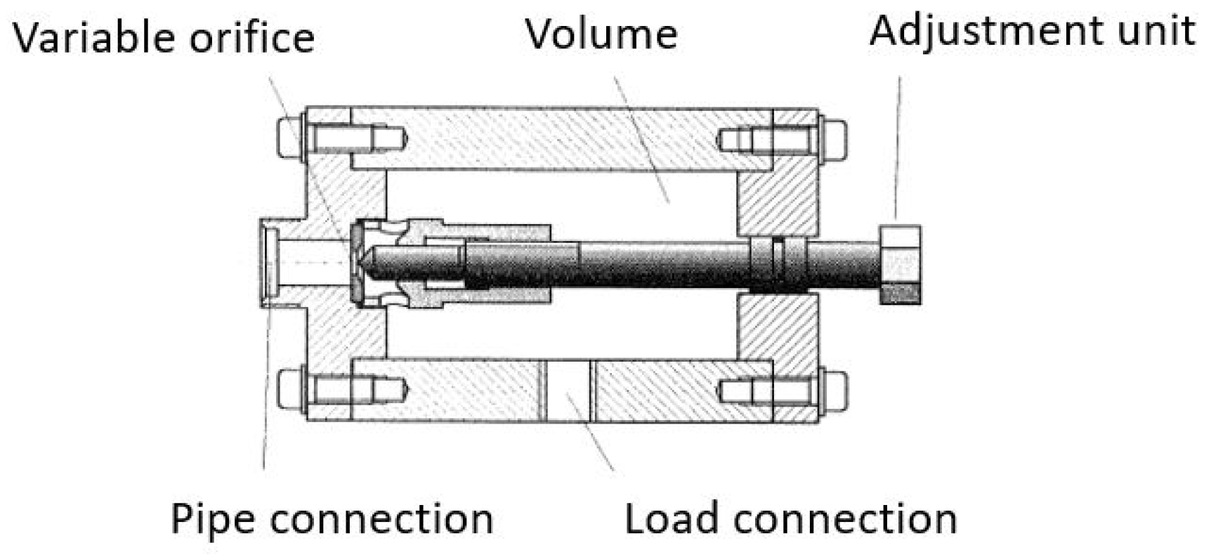
Figure 2.
Pressure history: (left) without reflection, (right) with reflection. [24]
Figure 2.
Pressure history: (left) without reflection, (right) with reflection. [24]
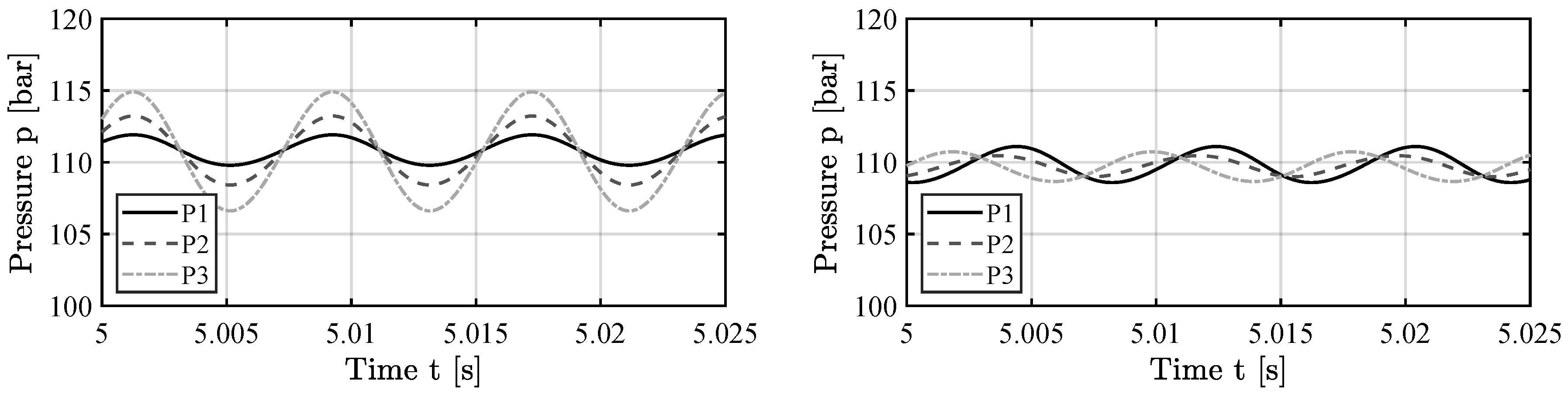
Figure 3.
The hydraulic circuit of the test rig.
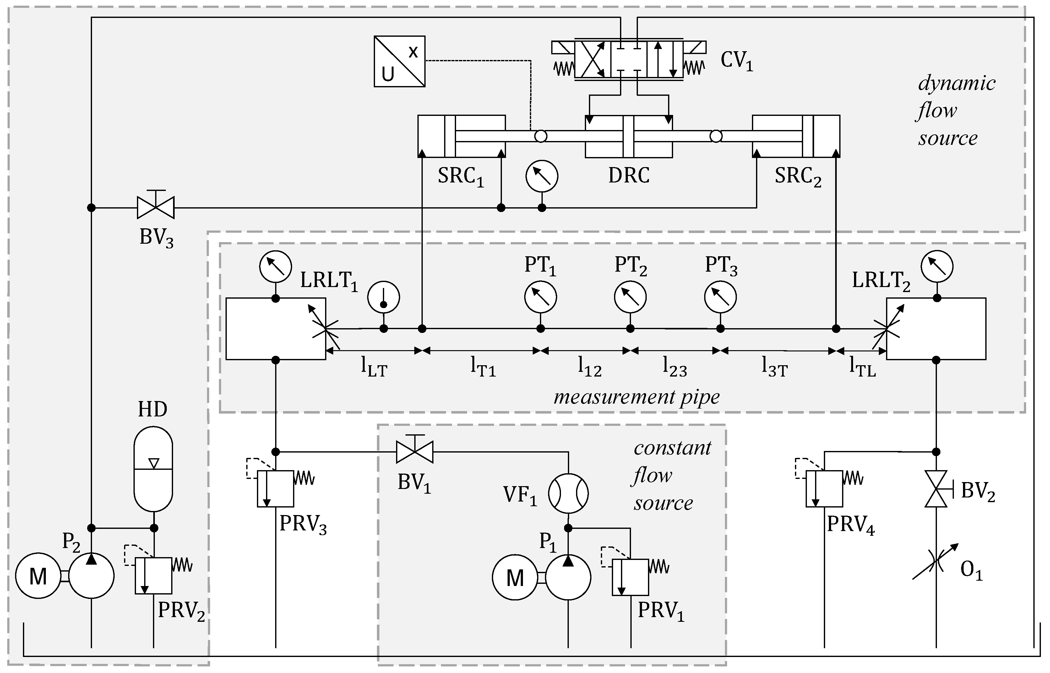
Figure 4.
Picture of the constructed test rig.
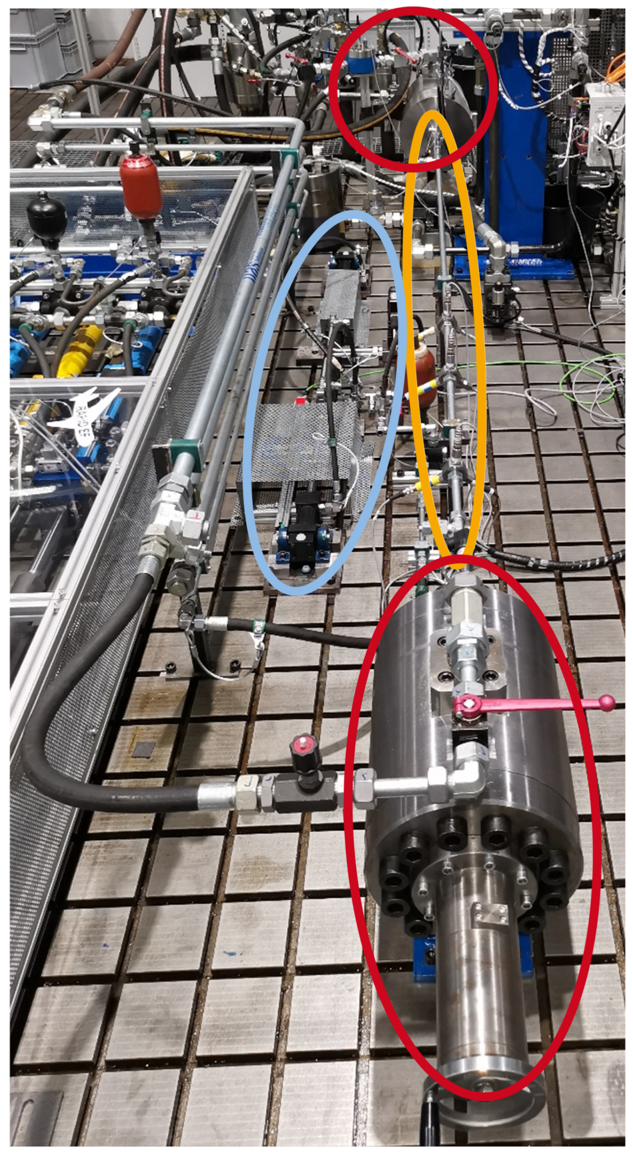
Figure 5.
Cross section of custom cutting ring fitting
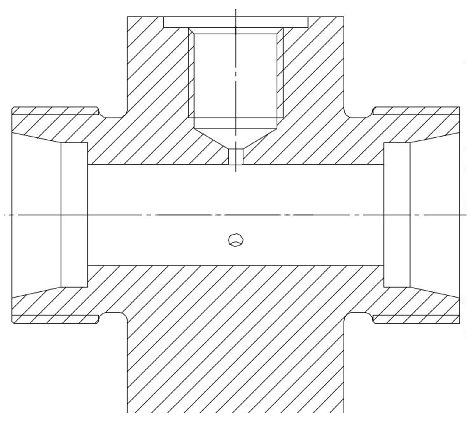
Table 2.
Mean errors and standard deviation for the tested frequencies and degrees of non-uniformity.
Table 2.
Mean errors and standard deviation for the tested frequencies and degrees of non-uniformity.
| Frequency f [Hz] | Degree of Non-uniformity [-] | Mean Error | Standard Deviation |
|---|---|---|---|
| 5 (Figure 6, Figure 7 and Figure 8) | , , | , , | , , |
| 10 (Figure 9, Figure 10 and Figure 11) | , , | , , | , , |
| 15 (Figure 12, Figure 13 and Figure 14) | , , | , , | , , |
Disclaimer/Publisher’s Note: The statements, opinions and data contained in all publications are solely those of the individual author(s) and contributor(s) and not of MDPI and/or the editor(s). MDPI and/or the editor(s) disclaim responsibility for any injury to people or property resulting from any ideas, methods, instructions or products referred to in the content. |
© 2024 by the authors. Licensee MDPI, Basel, Switzerland. This article is an open access article distributed under the terms and conditions of the Creative Commons Attribution (CC BY) license (http://creativecommons.org/licenses/by/4.0/).
Copyright: This open access article is published under a Creative Commons CC BY 4.0 license, which permit the free download, distribution, and reuse, provided that the author and preprint are cited in any reuse.


