
Submitted:
14 November 2024
Posted:
18 November 2024
You are already at the latest version
Abstract
Robot measurements for calibration and modelling are typically performed using a laser tracker. To measure three-dimensional positions, a Spherically-Mounted Retroreflector (SMR) is attached to the robot. Some researchers use adhesive bonds to attach the SMR, but this makes the positioning of the SMR inaccurate, unstable and unrepeatable, which affects the measurement itself and the traceability of the research results. We therefore investigated ways of attaching a SMR to the robot’s flange for accurate and repeatable measurements. At the same time, we observed measurement errors that occur when using a tool to attach a SMR to the flange. The solution that we developed is a 3D printed mount that can be attached to the flange. We evaluated the accuracy of the mount by measuring its eccentricity and the repeatability of placing the SMR in the mount. Our experiments showed that with an eccentricity radius of 0.35 mm and a repeatability inaccuracy of X=0.075 mm, Y=0.328 mm and Z=0.485 mm the mount has a sufficient accuracy to support calibration processes, traceability of research results and to replace adhesive bond.
Keywords:
Calibration
; Measurement error
; Repeatability
; Traceability
1. Introduction
Calibration and modelling data of robots often comes from high-precision position data from a laser tracker. For example, Lattanzi et al. use it to perform a calibration based on Tool Center Point (TCP) positions of a 6-axis robot arm [1]. Kong et al. use it to perform a kinematic calibration procedure and dynamically update the Denavit–Hartenberg (DH) parameters based on the laser tracker measurements [2]. Asif and Webb point out that some researchers and faculties are permanently attaching their SMRs, the corresponding tool for laser trackers, to their robots to perform calibrations and adaptations dynamically during the robot’s runtime [3]. And the company RoboDK uses its software in combination with three SMRs on a tool plate on the flange to calculate the six parameters that can be used to calibrate the TCP from the three coordinates of each SMR [4]. In each measurement scenario the SMR is attached to the robot. The literature describes a number of different approaches. Some researchers use a metal plate and monuments for the SMRs [5,6]. [2,4,7] fix their monuments with adhesive bond to a metal plate. Furthermore, [7] presents a SMR attachment based on a monument with strings. Asif and Webb use adhesive bond to attach a monument directly to the robot and place a SMR into it [3]. [8,9] use nests for the positioning of their SMRs and [5,10,11] place magnetic monuments on their robots in order to measure them. Companies such as MetrologyWorks also offer bolt-on monuments 1. The disadvantage of these monuments is that they are not robot specific. This means that the screw size does not fit to mount those monuments on a robot flange. The use of adapters can increase the inaccuracy of the fixation. In addition, these monuments are bulky and therefore not accessible to every laboratory. Santolaria et al. used an active target [12], which remains aligned with the laser tracker and enables the measurement of six dimensions through the provision of rotation information in addition to the and z coordinates. Some papers mention the position of the SMR for the measurement. The authors either use the robot flange [2,4,5,7,13,14,15,16], the links of the robot [7] or an end-effector attached to the robot flange [9,17,18,19,20,21,22,23,24,25].
None of the reviewed papers includes a standardised mount or a description of how the mount used in the experiments can be rebuilt. This way it is challenging to understand or replicate the findings of the papers and to perform the experiments again. It is hard to know exactly which mount was used, the mount is inaccessible or too expensive, or in the case of adhesive bond, it is unclear, where the SMR was placed exactly. Another complication with adhesive bond is the lack of repeatability when taking measurements for experiments. If the robot is used by more than one person in the laboratory, it is not possible to continue the experiment after removing the SMR for other uses, because the position of the reattached SMR varies greatly using adhesive bond.
This raises the questions, how a SMR can be attached to the robot’s flange for accurate and repeatable measurements and which errors can occur by using an attachment tool for an SMR.
On the following pages our solution in form of a 3D printed mount for attaching a laser tracker’s SMR to a robot flange is explained in detail. In combination with a SMR monument with back side magnet it can be used for flexible, repeatable and accurate measurements.
To prove its accuracy, we carried out two different experiments. First, we measured the eccentricity of the designed and printed mount. Then we also tested its repeatability. With our solution, we hope to offer a low-cost mount that can be used by a variety of laboratories and faculties to improve calibrations, research results and their traceability.
2. Materials and Methods
The mount for attaching a laser tracker’s SMR to a robot flange has been designed with the following requirements in mind. The mounting should be as close to the robot as possible to minimise the offset of the measuring point to the flange, which is also the standard TCP. The next requirement is that the designed mount should be easy to print on a standard 3D printer such as the Prusa i3 MK3S+. It should also use minimal material to be cost effective, lightweight and sustainable. The mount must comply with the ISO standard 9409-1-50-4-M6 for robot flanges, but without the directional pin. This makes it compatible with cobots such as the Universal Robots UR3e, UR5e and UR10e. The last requirement is that the mount centres a SMR monument for easy and repeatable SMR fixation with reduced eccentricity error.
2.1. Design of the Mount
Based on the requirements the mount in Figure 1 was constructed.
The model for 3D printing and construction details can be found on Thingiverse: https://www.thingiverse.com/thing:6792244.
The base of the mount is a cylinder with a diameter of 76.4mm and a height of 30mm. To attach the mount to a robot flange such as Universal Robots UR5e, a cylindrical hole with a diameter of 65mm and a depth of 5mm is added to the bottom of the base cylinder. This results in a remaining wall 5.7mm thick and 5mm high, which ensures a firm fit on the robot flange and prevents movement in either the x or y direction. The details are shown in the technical drawing (Figure 2).
The construction continues on the other side of the base cylinder with two cylindrical holes in the centre. The first one has a diameter of 20.2mm and a depth of 7.1mm to accommodate a 20 x 7 neodymium magnet. The second one is placed behind the first one and has a diameter of 4 and a depth of 5 to accommodate a threaded insert. The threaded insert is placed in the plastic of the 3D printed part and is used to secure the neodymium magnet with a screw.
In the next step a circular ring with an inner diameter of 40.6 and an outer diameter of 45, resulting in a wall thickness of 4.4, and a height of 5 is added to the base cylinder, starting from the centre. In combination with the neodymium magnet, it is used to fix a SMR monument with a magnetic back and prevents the monument from moving in either the x or y direction.
The final step of the construction is to create four holes for M6 screws. These are used to attach the mount to the robot flange. The holes are evenly spaced at 90 to each other on a circle with a radius of 25 from the centre. The holes start with a diameter of 10.5 and taper at 10 to a diameter of 6.7. A part of each hole removes a part of the previous wall for the SMR monument.
By following these construction steps, the mount is suitable for ISO standard 9409-1-50-4-M6 robot flanges and SMR monuments or drift nests for 1.1251.5inch SMRs or a diameter of 28.6.
2.2. Methods
When analysing the design of the SMR to robot flange mount, there are weaknesses in 3D printing the part. Every dimension and placement is calculated from the centre of the mount. A slight shift in the centre results in an eccentricity of the whole mount. The same thing happens if the holes for the M6 screws are shifted in relation to the circular ring for the SMR or vice versa. Although the mount was designed to reduce the eccentricity error, the use of a 3D printer to produce the part introduces a further inaccuracy.
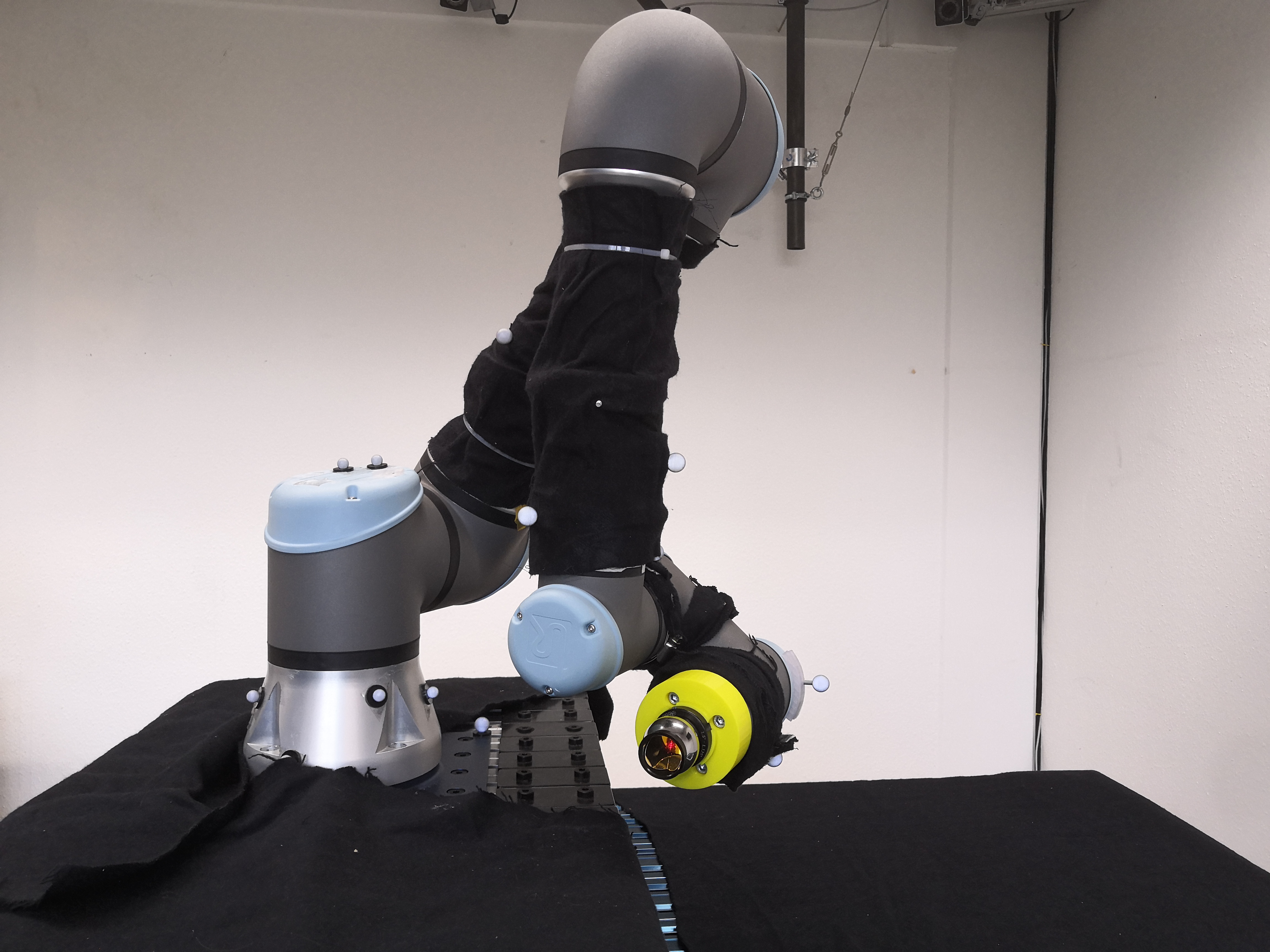
The following experiments were designed to measure the influence of the mount design and fabrication on laser tracker measurements. The first experiment focuses on a possible eccentricity of the mount. The second examines its repeatability. All experiments were carried out in the same laboratory using the same equipment and settings. For the high accuracy position measurements the laser tracker FARO Vantage E was used with a 1.5inch Standard Accuracy Break Resistant SMR from FARO with a gold coating, a range of 60 and a centring accuracy of 2. The designed mount was attached on a Universal Robots UR5e cobot. The cobot is shown in Figure 3, including the labelling of its axes. The measurement distance between the laser tracker and the SMR was 3. All experiments were carried out in a laboratory on the third floor of a university building during the university summer holidays, so there were no students and few staff around, which reduced movement and vibration of the floor, walls and ceiling. During the measurements the weather was warm and dry with a temperature of 2830 and humidity of 5055. The laser tracker was always warmed up for 45 minutes and a quick compensation and angle accuracy check was performed. The FARO CAM2 software was used for data acquisition and export. It collects positional values in a three-dimensional Cartesian space with the laser tracker as the origin. The orientation of the axes is defined by an internal home position and is constant.
The same setup was used for both experiments. The designed mount was attached to the robot flange facing the laser tracker. The SMR was placed inside the monument of the mount and aimed at the laser tracker. And the last wrist (Wrist 3) of the cobot was rotated so that a 360 rotation was possible. Figure 4 shows a visual representation of the settings.
2.2.1. Measurements of Eccentricity
In order to measure the eccentricity of the designed mount, the following experiment was carried out. The main idea is to rotate the mount and the SMR 360 using the last joint of the robot and measure it with the laser tracker. The joint is rotated in 10 increments and stopped to obtain a static measurement point. A laser tracker measurement is initiated. After a full rotation, 36 data points are available. The diameter of the resulting circle varies with eccentricity. To reduce the influence of the robot joint on the measurement, several positions are used for the rotation of the last joint. It was decided to use a rotation of 15 around the elbow joint for four times in order to have five measurement positions. Figure 5 shows this setup, including the device position of the laser tracker, its orientation vectors, the robot, the robot’s orientation vectors, the plane of rotation of the elbow joint and the measurement positions of the 360 rotations of the last robot joint. The robot’s wrist 3 is aligned so that the coordinate system of the TCP is aligned with the coordinate system of the laser tracker. The following applies:
The desired eccentricity, and therefore the measured circle, should be as small as possible. The smaller the eccentricity, the smaller the influence of the designed mount on the measurement values, as the alignment is irrelevant. Otherwise, the eccentricity radius will be added to each measurement, affecting the overall measurement accuracy.
2.2.2. Measurements of Repeatability
To measure the repeatability of the mount, the robot arm is kept static. The SMR is removed from the monument in the mount and re-positioned ten times. Each placement is measured by the laser tracker, resulting in ten measurement points.
In another experiment, the entire mount is removed from the robot’s flange and reinstalled. The screws are loosened completely and tightened again when it is remounted. This procedure is repeated five times and the SMR is always removed from the monument. The laser tracker measurements are carried out when the mount is fixed and the SMR is back in the monument, resulting in five measurement points.
Each of the two experiments is carried out in one setting, without breaks, to avoid changes in the measurement conditions and the setting.
3. Results
To give an idea of the accuracy of the experimental setup and the laser tracker FARO Vantage E used, the results of a baseline measurement are shown before the results of the designed experiments.
All measurement values are shown in nd visualized in coordinate systems with caling. The measurements include values from a right-handed Cartesian coordinate system with the laser tracker as the origin. For each value of the mean, median, min, max, the absolute value of the difference between min and max and the standard deviation are displayed. The standard deviation is calculated using the following equation:
3.1. Baseline Measurements
For the baseline measurement, 36 measurements were taken in a series in a static position without any changes to avoid measurement errors and to compare the standard measurement inaccuracy in the laboratory with the values given in the laser tracker data sheet. A discussion, comparison and classification of the measurements follows in Section 4. Figure 6 gives a visual representation of the scattering of the measurement points. For a clearer and more concise presentation, the decimal part is used for the tick labels, and the integer part is added to the respective axes variable. In Table 1 a summarized analysis of the measured values follows.
The raw data can be found on figshare under the following link: https://doi.org/10.6084/m9.figshare.27195387.v2.
3.2. Eccentricity Measurements
Multiple measurements were taken to determine the eccentricity of the designed and 3D printed mount. Five different locations were used for two independent 360° rotations with 36 measurements each. This gives a total of 360 measurements. Figure 7 shows one of the ten measurement runs and Figure 8 shows a 2D projection on the plane of the y- and z-axis of all eccentricity circles. The centre of all the measurements is moved to to compare them besides their different measurement locations. Table 2 shows the radii of the ten circles. The radii were calculated using the Python package circle-fitting-3d 3. The algorithm in this package is based on the blog post "Fitting a Circle to Cluster of 3D Points" by Miki [26]. It uses Singular Value Decomposition (SVD) and least squares to fit a circle to a 3D point cloud, which are the measured values. The fitted circle for measurement run Circle 1_2 is included in Figure 8. The raw data can be found on figshare under the following link: https://doi.org/10.6084/m9.figshare.27195483.v2.
Two sources of error that affect the eccentricity measurements are the unevenness of the 3D printed mount and the deviation from parallelism of the plane spanned by the and axes and the plane spanned by the and axes. The issue with an uneven surface is that measurement points are taken on a tumbling plane when the robot’s wrist 3 is rotated, which makes it challenging and unreliable to fit a circle into the point cloud. The issue of deviation from parallelism is that the measurement points must be projected onto the appropriate plane in order to fit a circle into them. Although the underlying algorithm of circle-fitting-3d is designed to address this challenge, a projection to the -plane of the laser tracker is a more reliable approach. To specify the magnitude of the errors, they were measured. Therefore ten measurement points on the monument of the mount were taken and analysed. The planarity of the printed mount is 0.014 and the angle between the and plane and the and plane is 0.115. These errors must be considered when interpreting the values in Table 2. The raw data can be found on figshare under the following link: https://doi.org/10.6084/m9.figshare.27468399.v1.
3.3. Repeatability Measurements
The ten measurements of the first experiment to define the repeatability of the SMR placement in the monument of the mount are visualised in Figure 9 and analysed in Table 3. The five values of the second experiment, where the whole mount is repeatedly mounted and dismounted, are visualised in Figure 10 and analysed in Table 4. The raw data can be found on figshare under the following link: https://doi.org/10.6084/m9.figshare.27195540.v2.
4. Discussion
This section offers a comprehensive analysis of the results presented in Section 3. It compares these results with the technical specifications, baseline data, and established requirements.
4.1. Baseline
The baseline measurements are used to determine the accuracy of the measurement setup in the laboratory with the used laser tracker FARO Vantage E, the SMR and the environmental influence. The measured values (Table 1) are compared with the technical specifications provided by FARO 4:
- Distance-Error for the used laboratory settings (3 distance between laser tracker and SMR):
- Angle-Error for the used laboratory settings (3 distance between laser tracker and SMR):
The distance and angle errors of the baseline measurement are calculated from the absolute value of the difference between the min and max value of the measured values for each axis:
Table 5 shows a comparison between the theoretical measurement accuracy and the actual baseline values.
and are within the expected error (maximum permissible error) of the data sheet. exceeds the maximum permissible error for angle errors from the data sheet (). But only by 0.013, so it is still in the same order of magnitude. And the standard deviation of [uncertainty-mode=separate]-556.389(0.0088) is in line with the maximum permissible error. Overall, the baseline measurements show that the laboratory environment can be used for accurate and reliable measurements.
4.2. Eccentricity
To contextualise the eccentricity error introduced by the designed mount, the eccentricity radii (Table 2) of the experiment in Section 2.2.1 are compared with the baseline and desired accuracies mentioned in other papers [1,3,4]. The highest measured eccentricity radius is 0.353. This results in an eccentricity diameter of 0.706, which means that a measurement point, which should have exactly the same x,y,z coordinates for each measurement, deviates in the worst case by 0.706. Compared to the baseline measurement, where the largest deviation is 0.048, which shows how accurate measurements can be, this is times. So instead of an accuracy in the hundredths of a millimetre range, one dimension is lost and an accuracy in the tenths of a millimetre range is achieved. In comparison, Asif and Web worked on an error correction in the range of 0.02 [3], which is in the range of the distance error of the FARO Vantage E laser tracker used. The radius introduced by our new tool is one order of magnitude higher. Lattanzi et al. worked on a robot positioning accuracy of up to 0.1 for their considered task [1]. This value is still exceeded by a factor of 7 in the worst case by our mount. Finally, RoboDK has developed a calibration procedure for their software which supports an accuracy of 0.05 for small robots and 0.15 for medium sized robots [4]. Our tool is not suitable for such high accuracy jobs. However, although the worst case of 0.705 deviation is insufficient, it is not very likely. Depending on the measurement method and the trajectory, the radius is not added to the measurements, because the eccentricity does not come into play. An alternative approach would be to measure eccentricity circles at each desired measurement position and use the centre of the circle as the measurement point.
4.3. Repeatability
To provide a context for the repeatability accuracies of the mount, it is compared to the baseline measurement. Therefore the measured values for the x,y and z deviations are compared in the Table 6. The distance and angle errors are calculated in the same way as for the baseline measurements using the equations 7, 8 and 9.
As expected, the baseline measurement has the smallest deviations, followed by the repeatability measurement of SMR in monument placement and finally the repeatability measurement of mounting and dismounting of the mount. The factors of inaccuracy between baseline (BaseM) and SMR in monument placement (RepM1) are:
However, despite the highest factor between baseline and repeatability measurement, the x-axis still has the lowest deviation of the measurement points () of all axes. A comparison between the baseline (BaseM) and the mounting and dismounting of the mount (RepM2) gives the following inaccuracy factors:
To put the high factor for the z-axis into perspective, is relatively low, and the for the z-value of the mounting and dismounting of the mount is relatively high compared to the x- and y-axis. However, they are still in the same order of magnitude. The difference between the y- and z-values of the SMR in monument placement and the mounting and dismounting of the mount can be explained by microshifts of the robot during the attachment of the mount, which add up to the inaccuracy of the designed mount. To prove this, a further experiment was carried out to measure the shift of the robot during the attachment of the mount. Therefore the mount was attached to the robot flange, the SMR was placed in the monument and an initial position was measured with the laser tracker. Fastening was then simulated by pressing an Allen key into each of the four screw holes with a force of 25 and taking a measurement for each. The results are shown in the Table 7 and the raw data can be found on figshare under the following link: https://doi.org/10.6084/m9.figshare.27604596.v1. The following equations were used to calculate the maximum shift using the absolute value of the maximum difference between the initial pose and the four measurements :
Taking the maximum shift into account the comparison between the baseline (BaseM) and the mounting and dismounting of the mount (RepM2) in the equations 13, 14 and 15 can be recalculated with the following equations:
If the microshifts of the robot during the installation of the mount are taken into account, the factor between the baseline and the repeatability measurement for the x-axis hardly changes, the factor for the y-axis is reduced by and the factor for the z-axis is reduced by . Another result of the microshift experiment was the self-healing mechanism of the robot. After 30, the position of the robot was almost the same as the initial position. This should be taken into account for more accurate measurements after the mount has been attached. In addition to the comparison with the baseline measurement, a comparison with the eccentricity results is also interesting. The eccentricity radius can be compared with and as they lie on the same plane. The highest eccentricity radius is 0.353 ( diameter), is 0.328 and is 0.485. So the deviation introduced by the eccentricity diameter is and higher. All of the values are the worst case values. The standard deviation was lower by around about 50. Combined the eccentricity and repeatability errors add an inaccuracy of in the worst case. This is something to consider when using the mount for high accuracy applications as it affects measurements.
5. Conclusions
Despite its potential inaccuracies in eccentricity and repeatability, the designed mount for attaching a SMR to a robot flange offers an easy to build, affordable and accessible solution for robot measurements using laser trackers. It supports the repeatability of research experiments and measurements, improving the traceability of results. It enables research laboratories to verify the results of colleagues and fellow researchers. The success of the mount depends largely on its distribution and use in laboratories. The more users there are, the more comprehensible and reproducible the results based on this measuring instrument will be. The next steps are to further improve the design to reduce eccentricity and increase repeatability. Other materials will be compared to the 3D printed mount, such as CNC machined aluminium or steel. The mount could be extended to rotate the SMR to keep it aligned with the laser tracker as the robot moves. This could be done by adding a bearing and changing the design of the mount. Or the mount could be extended to hold up to four SMRs monuments for a six dimensional perception of the mount with the position and orientation of the robot flange in .
Author Contributions
Conceptualization, F.S., S.M.; methodology, F.S.; software, F.S.; validation, F.S., S.M.; formal analysis, F.S., M.G.; investigation, F.S.; resources, M.S.; data curation, F.S.; writing—original draft preparation, F.S.; writing—review and editing, S.M., M.S., M.G.; visualization, F.S., S.M.; supervision, M.S., M.G.; project administration, F.S., M.G.; funding acquisition, M.S. All authors have read and agreed to the published version of the manuscript.
Funding
This research received no external funding.
Institutional Review Board Statement
Not applicable.
Informed Consent Statement
Not applicable.
Data Availability Statement
The original data presented in the study are openly available in figshare at https://doi.org/10.6084/m9.figshare.27195387.v2, https://doi.org/10.6084/m9.figshare.27195483.v2, https://doi.org/10.6084/m9.figshare.27468399.v1, https://doi.org/10.6084/m9.figshare.27195540.v2 and https://doi.org/10.6084/m9.figshare.27604596.v1.
Conflicts of Interest
The authors declare no conflicts of interest. The funders had no role in the design of the study; in the collection, analyses, or interpretation of data; in the writing of the manuscript; or in the decision to publish the results.
Abbreviations
The following abbreviations are used in this manuscript:
| BaseM | Baseline Measurement |
| DH | Denavit–Hartenberg |
| RepM1 | Repeatability Measurement 1 |
| RepM2 | Repeatability Measurement 2 |
| SMR | Spherically-Mounted Retroreflector |
| SVD | Singular Value Decomposition |
| TCP | Tool Center Point |
References
- Lattanzi, L.; Cristalli, C.; Massa, D.; Boria, S.; Lépine, P.; Pellicciari, M. Geometrical Calibration of a 6-Axis Robotic Arm for High Accuracy Manufacturing Task. The International Journal of Advanced Manufacturing Technology, 111, 1813–1829. [CrossRef]
- Kong, Y.; Yang, L.; Chen, C.; Zhu, X.; Li, D.; Guan, Q.; Du, G. Online kinematic calibration of robot manipulator based on neural network. Measurement, 238, 115281. [CrossRef]
- Asif, S.; Webb, P. Realtime Calibration of an Industrial Robot. Applied System Innovation, 5, 96. [CrossRef]
- RoboDK. Robot calibration with a laser tracker. https://robodk.com/doc/en/Robot-Calibration-LaserTracker.html, accessed on 2024-08-13.
- Nubiola, A.; Bonev, I.A. Absolute Calibration of an ABB IRB 1600 Robot Using a Laser Tracker. Robotics and Computer-Integrated Manufacturing 2013, 29, 236–245. [Google Scholar] [CrossRef]
- Nubiola, A.; Slamani, M.; Joubair, A.; Bonev, I.A. Comparison of Two Calibration Methods for a Small Industrial Robot Based on an Optical Cmm and a Laser Tracker. Robotica 2013, 32, 447–466. [Google Scholar] [CrossRef]
- Ferrarini, S.; Bilancia, P.; Raffaeli, R.; Peruzzini, M.; Pellicciari, M. A method for the assessment and compensation of positioning errors in industrial robots. [CrossRef]
- Qiao, G.; Weiss, B.A. Quick Health Assessment for Industrial Robot Health Degradation and the Supporting Advanced Sensing Development. J. Manuf. Syst. 2018, 48, 51–59. [Google Scholar] [CrossRef] [PubMed]
- Wang, Z.; Zhang, R.; Keogh, P. Real-Time Laser Tracker Compensation of Robotic Drilling and Machining. Journal of Manufacturing and Materials Processing 2020, 4, 79. [Google Scholar] [CrossRef]
- Xiong, G.; Ding, Y.; Zhu, L. Stiffness-Based Pose Optimization of an Industrial Robot for Five-Axis Milling. Robotics and Computer-Integrated Manufacturing 2019, 55, 19–28. [Google Scholar] [CrossRef]
- Yin, S.; Ren, Y.; Zhu, J.; Yang, S.; Ye, S. A Vision-Based Self-Calibration Method for Robotic Visual Inspection Systems. Sensors 2013, 13, 16565–16582. [Google Scholar] [CrossRef]
- Santolaria, J.; Conte, J.; Ginés, M. Laser Tracker-Based Kinematic Parameter Calibration of Industrial Robots by Improved CPA Method and Active Retroreflector. The International Journal of Advanced Manufacturing Technology 2012, 66, 2087–2106. [Google Scholar] [CrossRef]
- Tian, W.; Zeng, Y.; Zhou, W.; Liao, W. Calibration of Robotic Drilling Systems with a Moving Rail. Chinese Journal of Aeronautics 2014, 27, 1598–1604. [Google Scholar] [CrossRef]
- Vincze, M.; Prenninger, J.; Gander, H. A Laser Tracking System to Measure Position and Orientation of Robot End Effectors Under Motion. The International Journal of Robotics Research 1994, 13, 305–314. [Google Scholar] [CrossRef]
- Yang, K.; Yang, W.; Cheng, G.; Lu, B. A New Methodology for Joint Stiffness Identification of Heavy Duty Industrial Robots with the Counterbalancing System. Robotics and Computer-Integrated Manufacturing 2018, 53, 58–71. [Google Scholar] [CrossRef]
- Zhenhua, W.; Hui, X.; Guodong, C.; Rongchuan, S.; Sun, L. A Distance Error Based Industrial Robot Kinematic Calibration Method. Industrial Robot: An International Journal 2014, 41, 439–446. [Google Scholar] [CrossRef]
- Yuan, P.; Chen, D.; Wang, T.; Cao, S.; Cai, Y.; Xue, L. A Compensation Method Based on Extreme Learning Machine to Enhance Absolute Position Accuracy for Aviation Drilling Robot. Advances in Mechanical Engineering 2018, 10, 1687814018763411. [Google Scholar] [CrossRef]
- Jo, M.; Chung, M.; Kim, K.; Kim, H.Y. Improving Path Accuracy and Vibration Character of Industrial Robot Arms with Iterative Learning Control Method. International Journal of Precision Engineering and Manufacturing. [CrossRef]
- Ouyang, J.F.; Liu, W.; Qu, X.H.; Yan, Y. Industrial Robot Error Compensation Using Laser Tracker System. Key Engineering Materials 2008, 381–382, 579–582. [Google Scholar] [CrossRef]
- Kamali, K.; Joubair, A.; Bonev, I.A.; Bigras, P. Elasto-geometrical calibration of an industrial robot under multidirectional external loads using a laser tracker. 2016 IEEE International Conference on Robotics and Automation (ICRA). IEEE, 2016, pp. 4320–4327. [CrossRef]
- Bai, Y.; Zhuang, H.; Roth, Z. Experiment study of PUMA robot calibration using a laser tracking system. Proceedings of the 2003 IEEE International Workshop on Soft Computing in Industrial Applications, 2003. SMCia/03. IEEE, SMCIA-03, pp. 139–144. [CrossRef]
- Yan, Y.; Ouyang, J.; Liu, W.; Deng, X.; Wang, X. Error Correction for the Tracking Mirror. 2008 International Conference on Intelligent Computation Technology and Automation (ICICTA). IEEE, 2008, Vol. 1, pp. 1048–1051. [CrossRef]
- Cvitanic, T.; Melkote, S.; Balakirsky, S. Improved state estimation of a robot end-effector using laser tracker and inertial sensor fusion. CIRP Journal of Manufacturing Science and Technology 2022, 38, 51–61. [Google Scholar] [CrossRef]
- Guerin, D.; Caro, S.; Garnier, S.; Girin, A. Optimal measurement pose selection for joint stiffness identification of an industrial robot mounted on a rail. 2014 IEEE/ASME International Conference on Advanced Intelligent Mechatronics. IEEE, 2014, pp. 1722–1727. ISSN: 2159-6255. [CrossRef]
- Lau, K.; Hocken, R.; Haynes, L. Robot Performance Measurements Using Automatic Laser Tracking Techniques. Robot. Comput.-Integr. Manuf. 1985, 2, 227–236. [Google Scholar] [CrossRef]
- Miki. Fitting a Circle to Cluster of 3D Points. https://meshlogic.github.io/posts/jupyter/curve-fitting/fitting-a-circle-to-cluster-of-3d-points/, accessed on 2024-08-20.
| 1 | |
| 2 | Technical data sheet SMR: https://media.faro.com/-/media/Project/FARO/FARO/FARO/Resources/2021/01/15/22/46/Tech-Sheet-FARO-Laser-Tracker-Targets-ENG.pdf?rev=53837c1533274c969ac6e1d10adcd612 (accessed on 2024-09-30) |
| 3 |
https://github.com/CristianoPizzamiglio/circle-fitting-3d (accessed on 2024-09-30) |
| 4 | Technical data sheet FARO Vantage S/E: https://media.faro.com/-/media/Project/FARO/FARO/FARO/Resources/2_TECH-SHEET/FARO-Vantage-Laser-Trackers/TechSheet_Vantage_DEU.pdf?rev=ca774471ef1d40e983a00b6f9e92da83 (accessed on 2024-09-30) |
Figure 1.
3D visualisation and application of the designed mount.
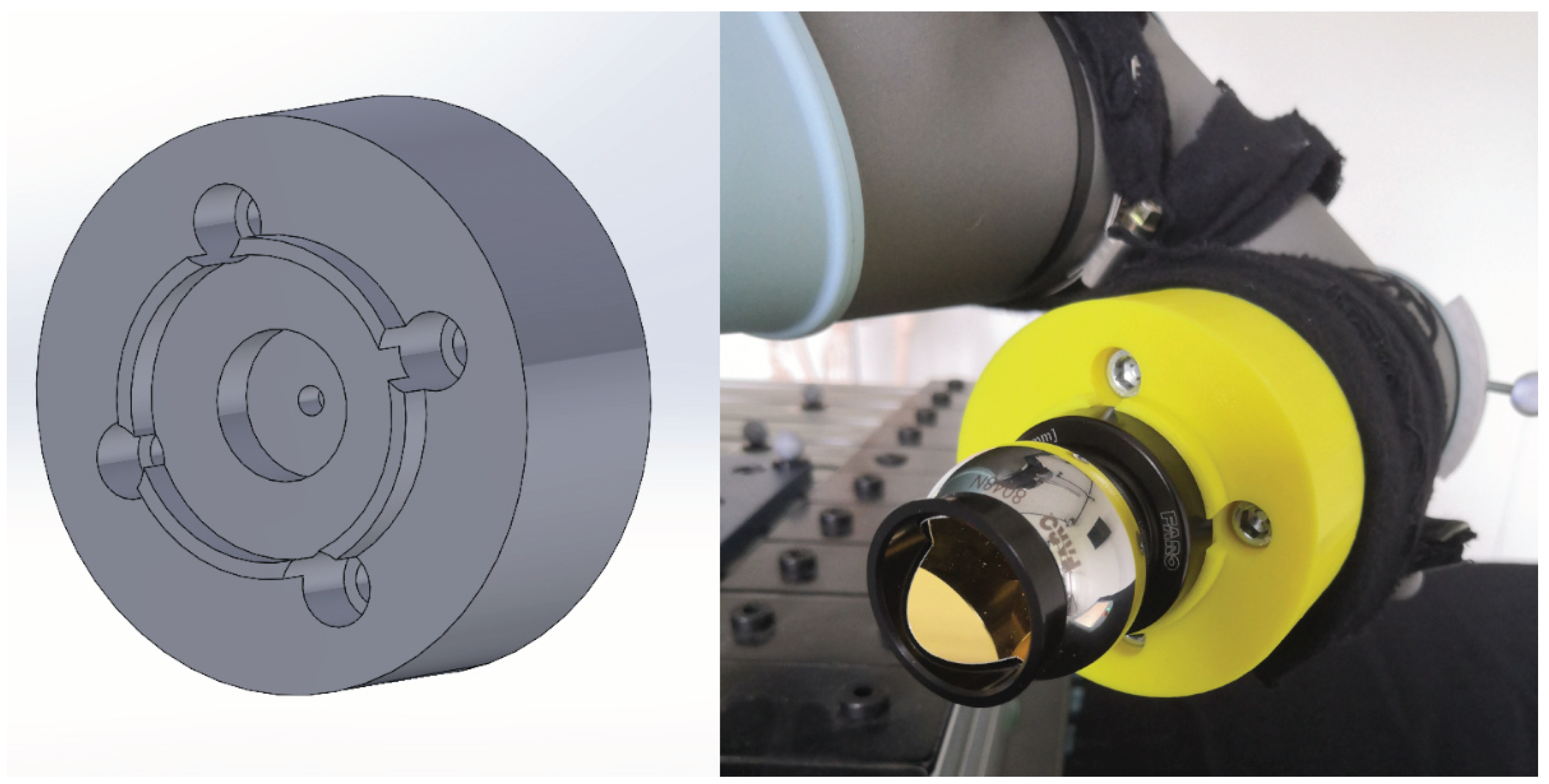
Figure 2.
Technical drawing of the designed mount with dimensions in mm.
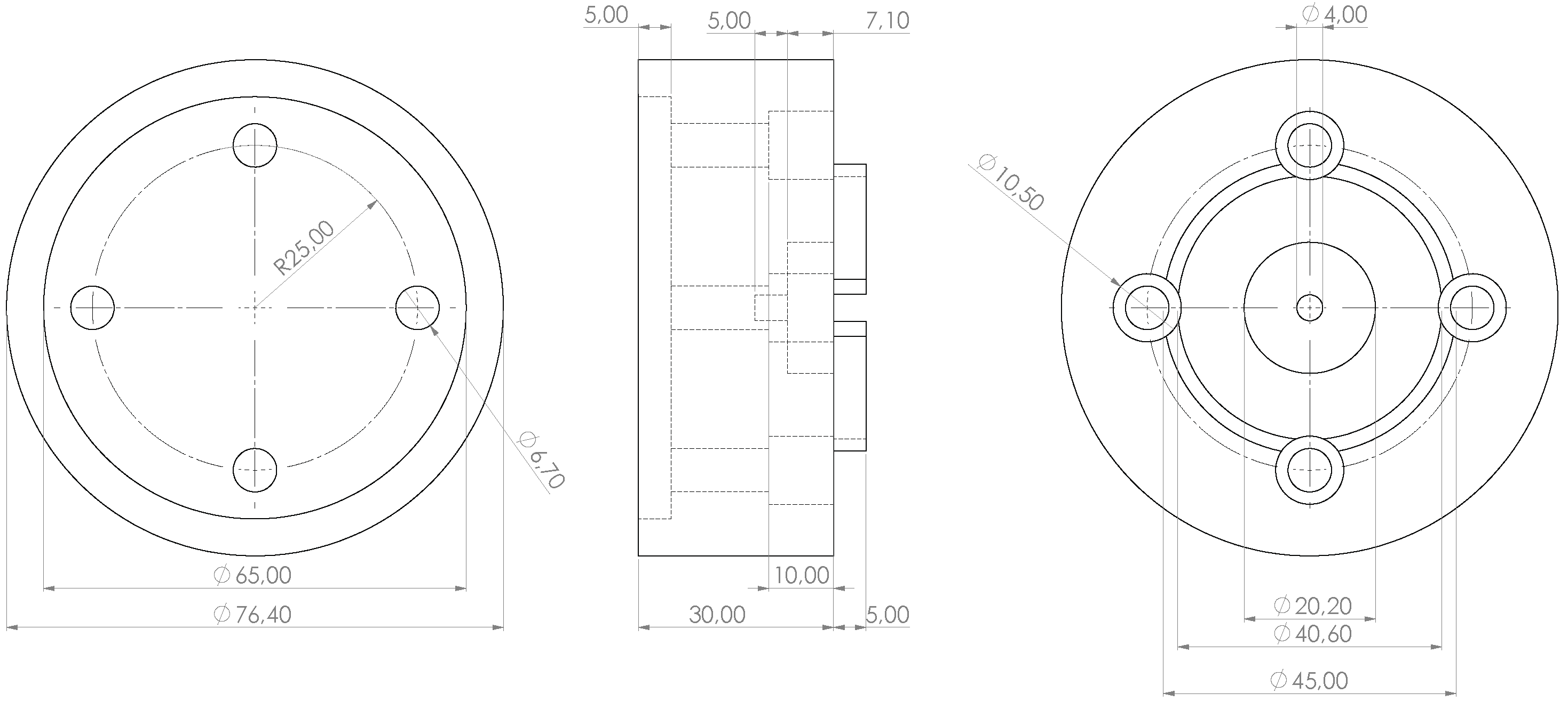
Figure 3.
Universal Robots UR5e with labelled axes.
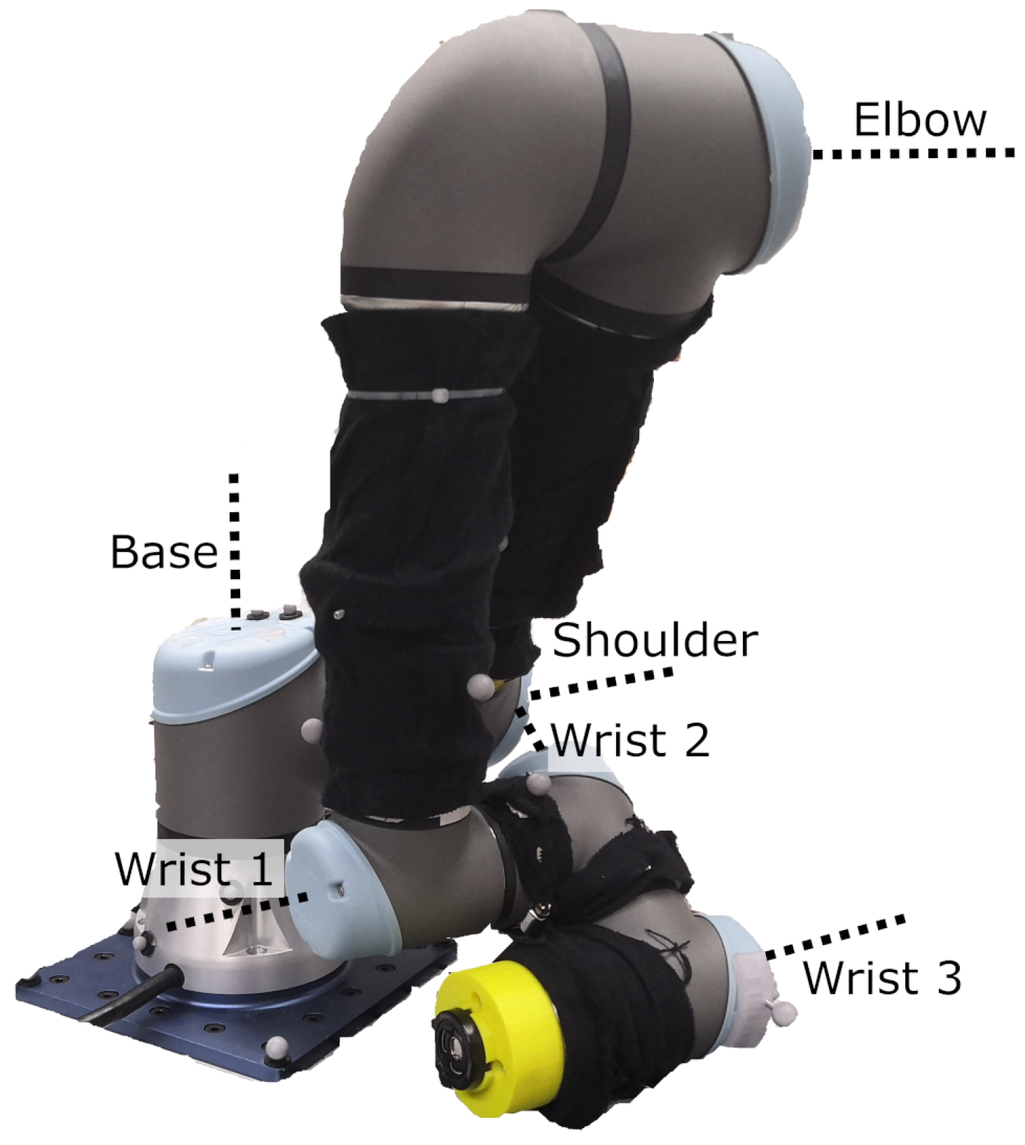
Figure 4.
Laboratory setting for measurements of mount errors.
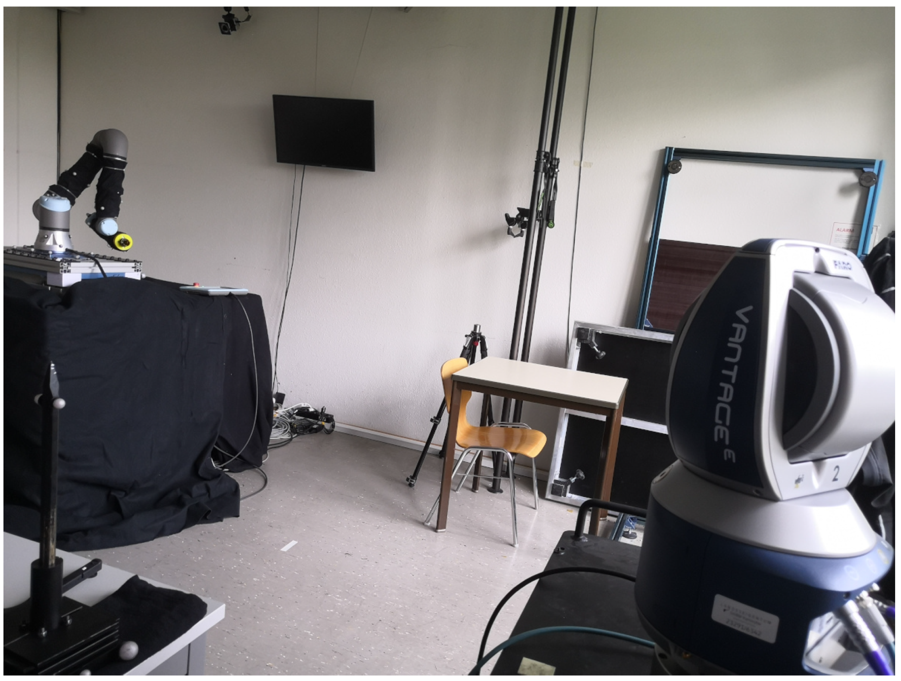
Figure 5.
Visual representation of the experimental setup for the eccentricity measurement including laser tracker position, robot, their orientation vectors and five measurement positions around the elbow joint.
Figure 5.
Visual representation of the experimental setup for the eccentricity measurement including laser tracker position, robot, their orientation vectors and five measurement positions around the elbow joint.
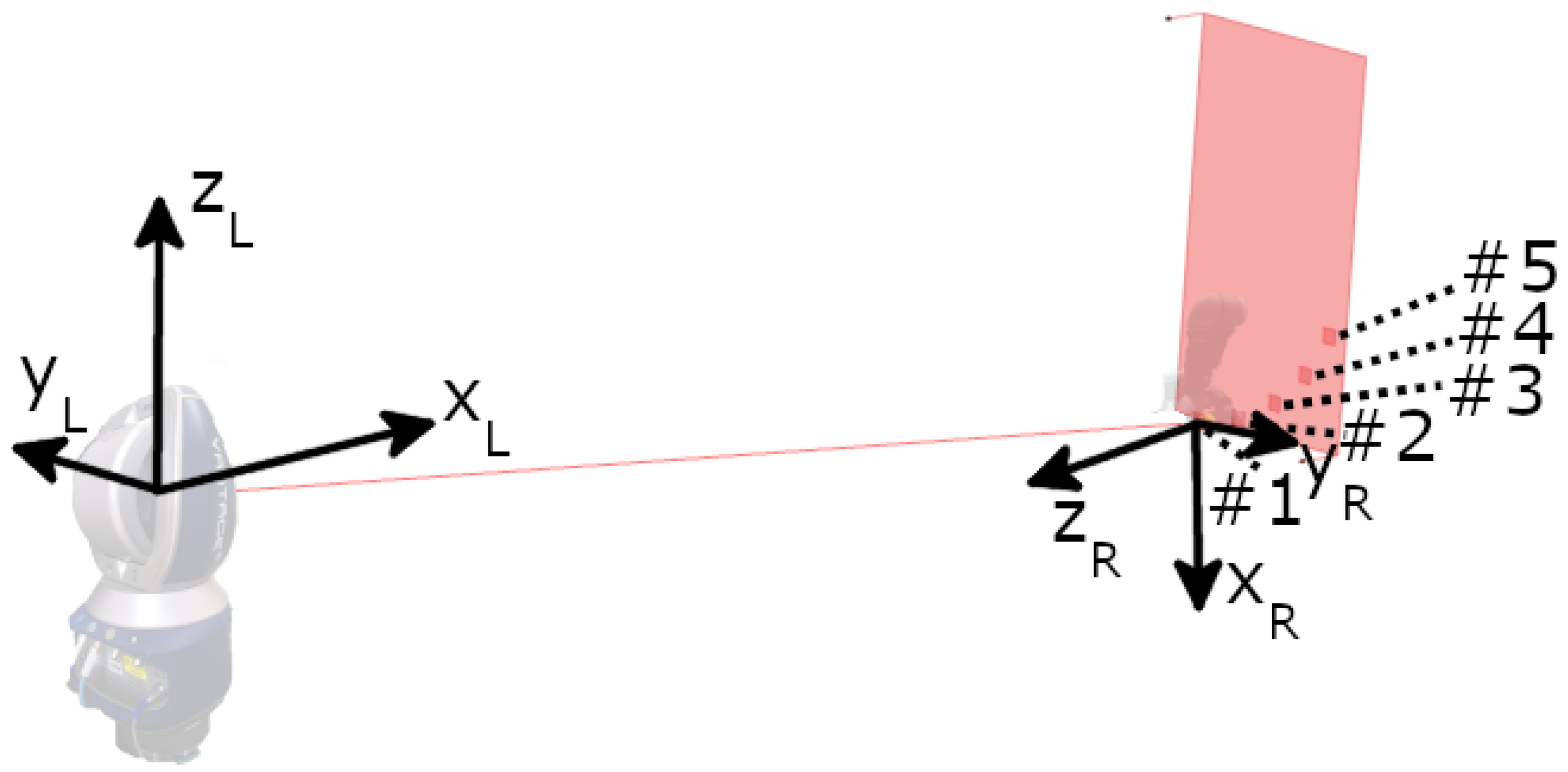
Figure 6.
Scatter plot of the 36 static measurement points which define the baseline.
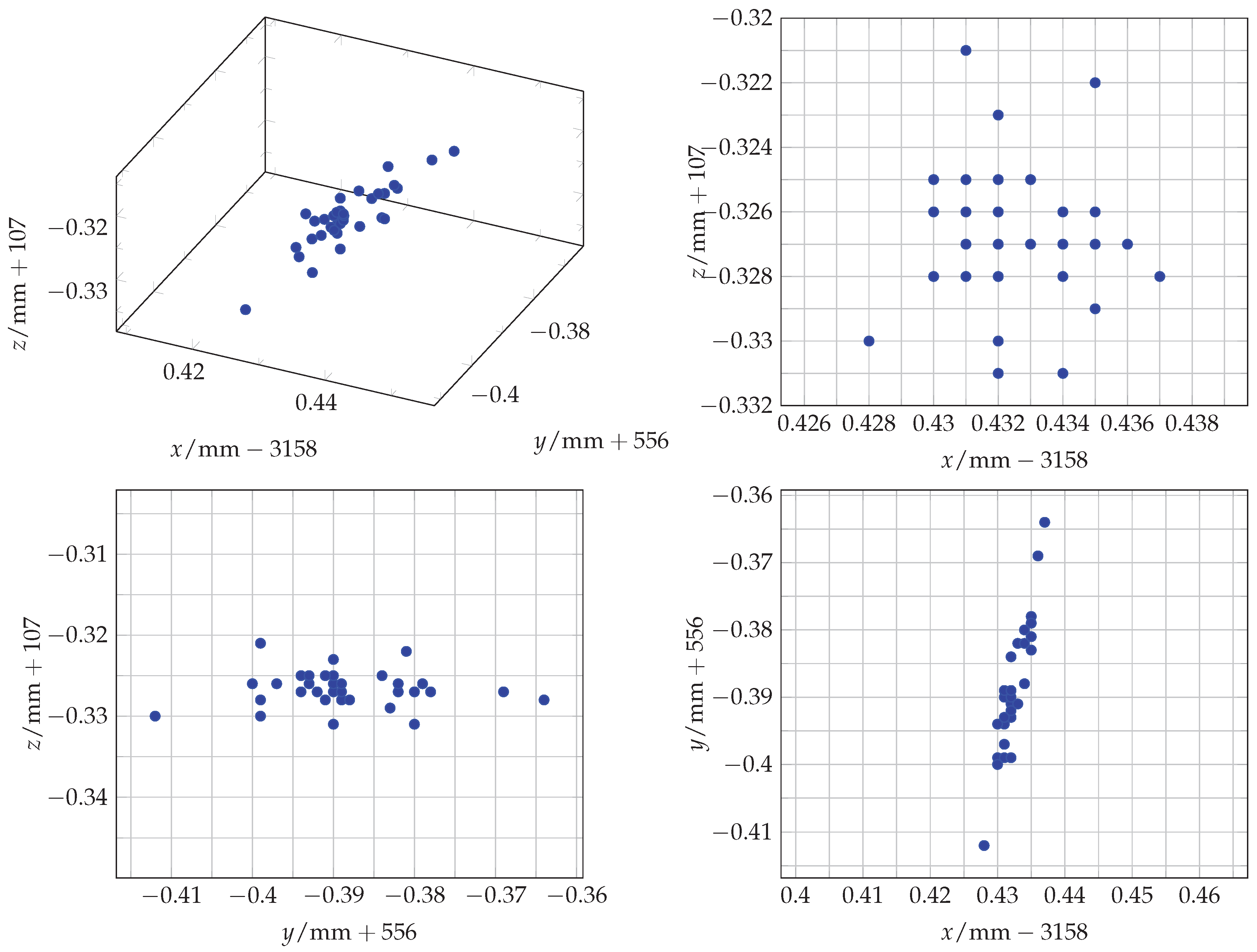
Figure 7.
Scatter plot of the 36 measurement points of one eccentricity circle (Circle 1_1).
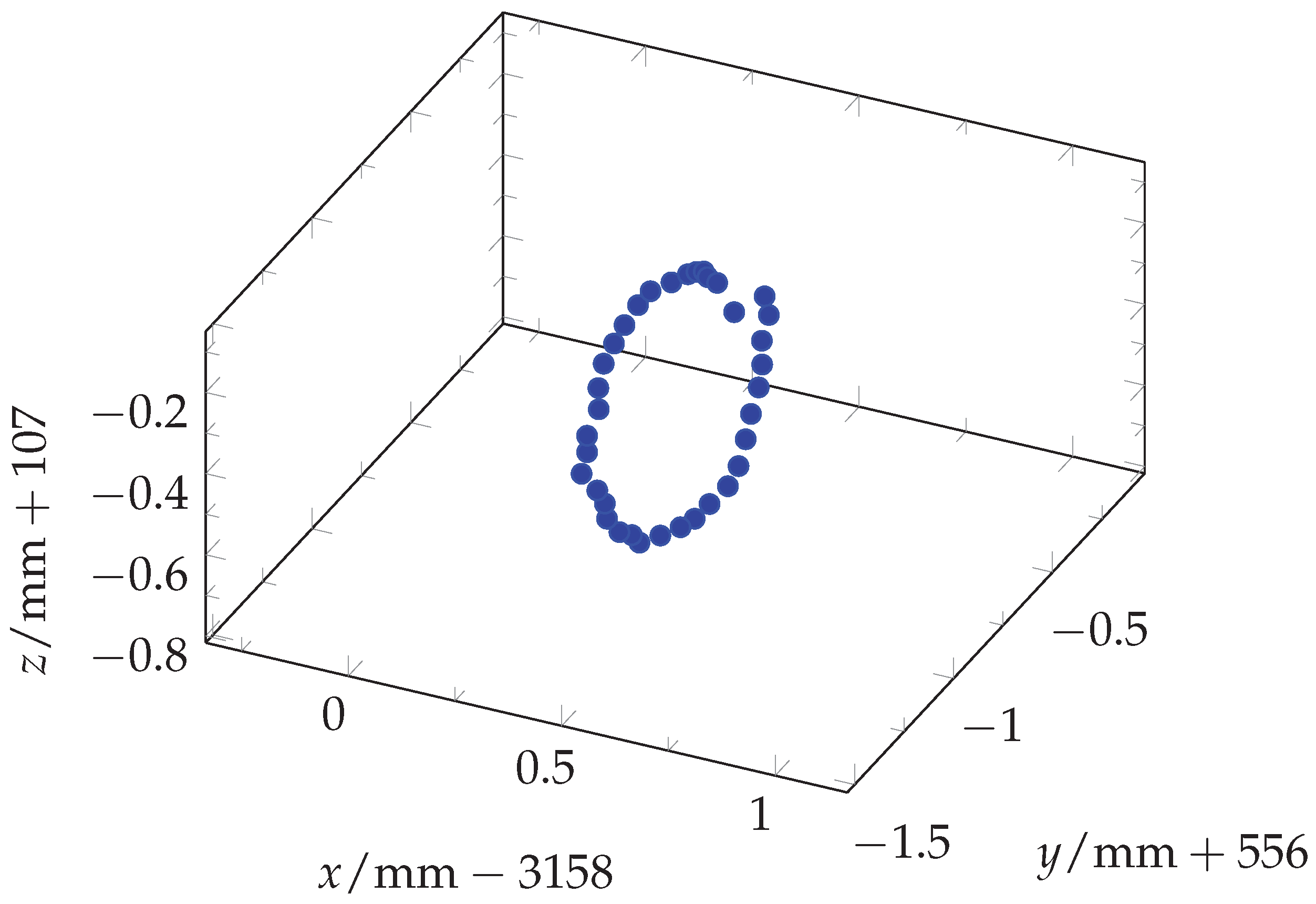
Figure 8.
2D projection of the 10 eccentricity circles with 36 measurement points each, moved to the centre , and fitted circle for Circle 1_2 with radius .
Figure 8.
2D projection of the 10 eccentricity circles with 36 measurement points each, moved to the centre , and fitted circle for Circle 1_2 with radius .
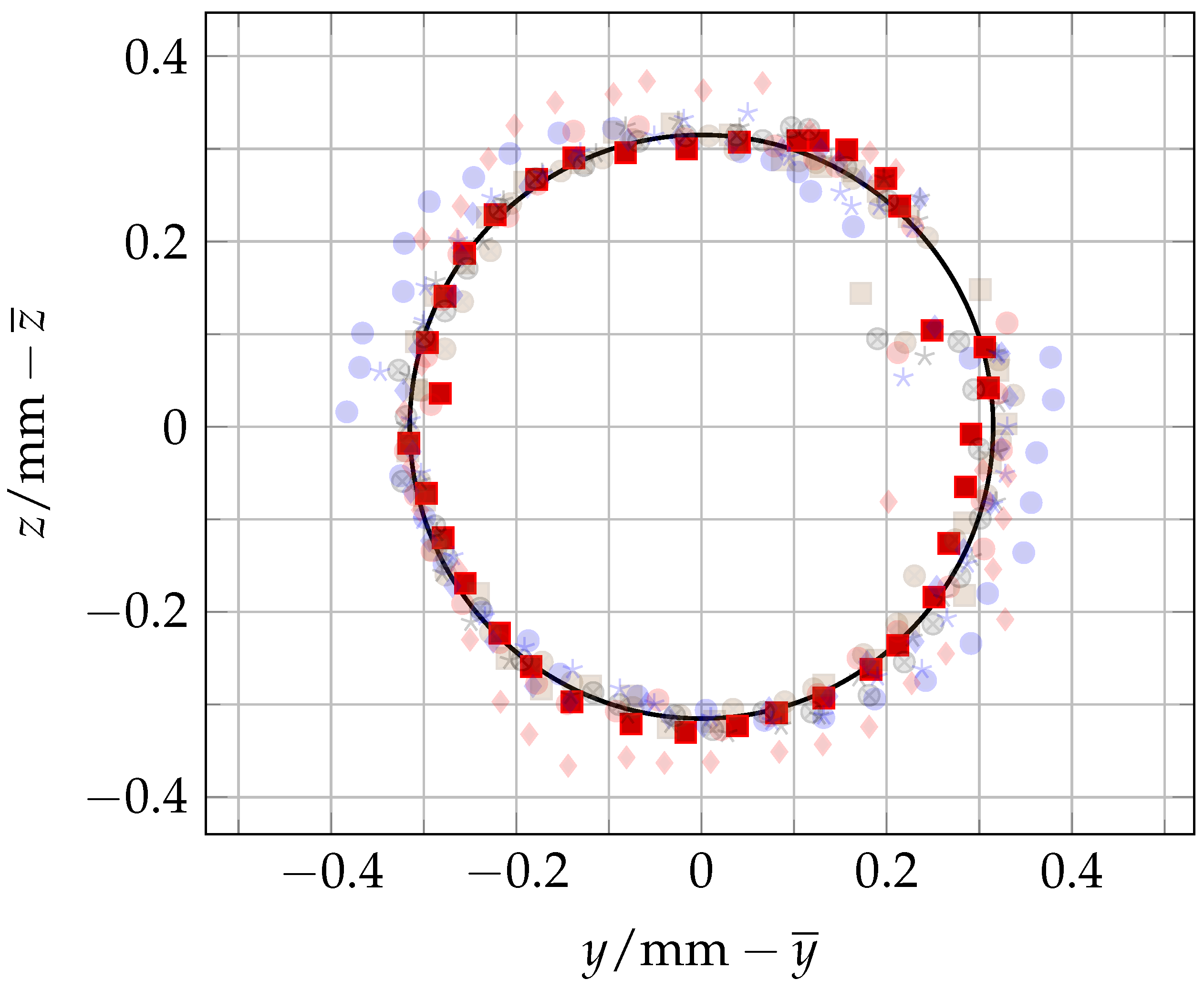
Figure 9.
Scatter plot of the 10 measurement points of placing the SMR repeatedly in the monument.
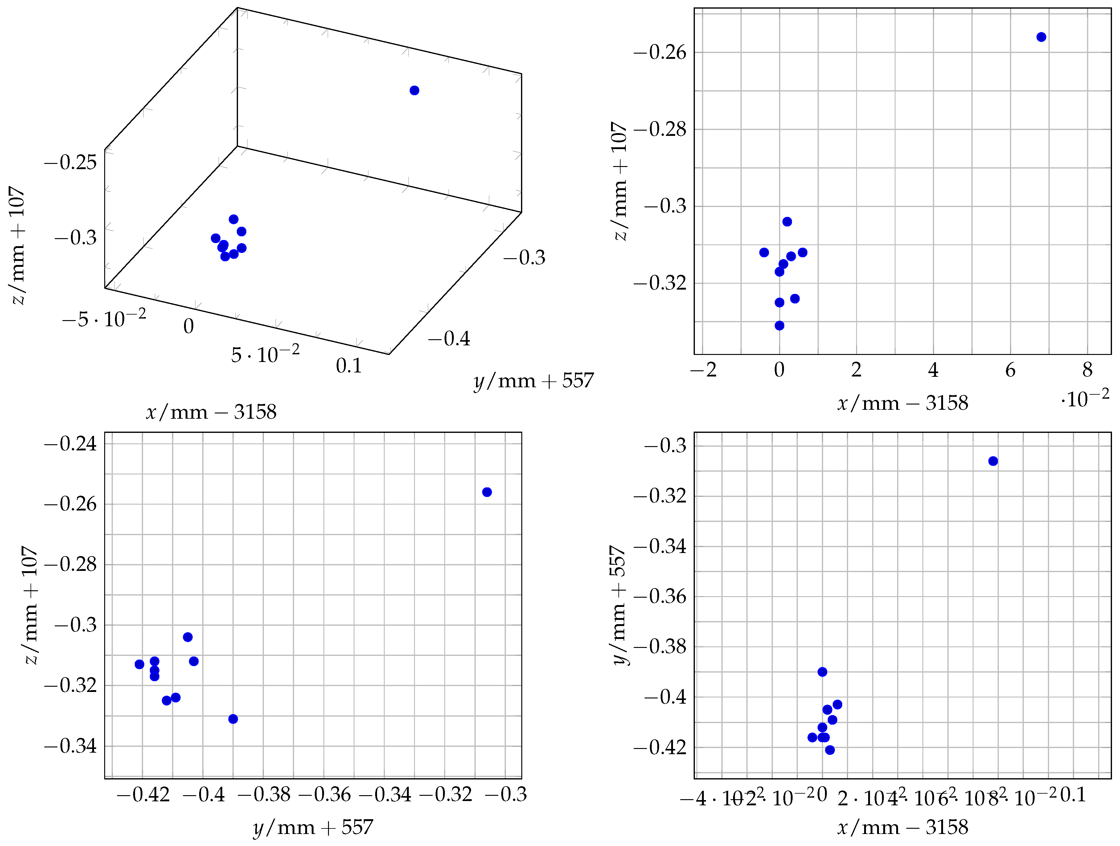
Figure 10.
Scatter plot of the 5 measurement points of mounting and dismounting the mount repeatedly.
Figure 10.
Scatter plot of the 5 measurement points of mounting and dismounting the mount repeatedly.
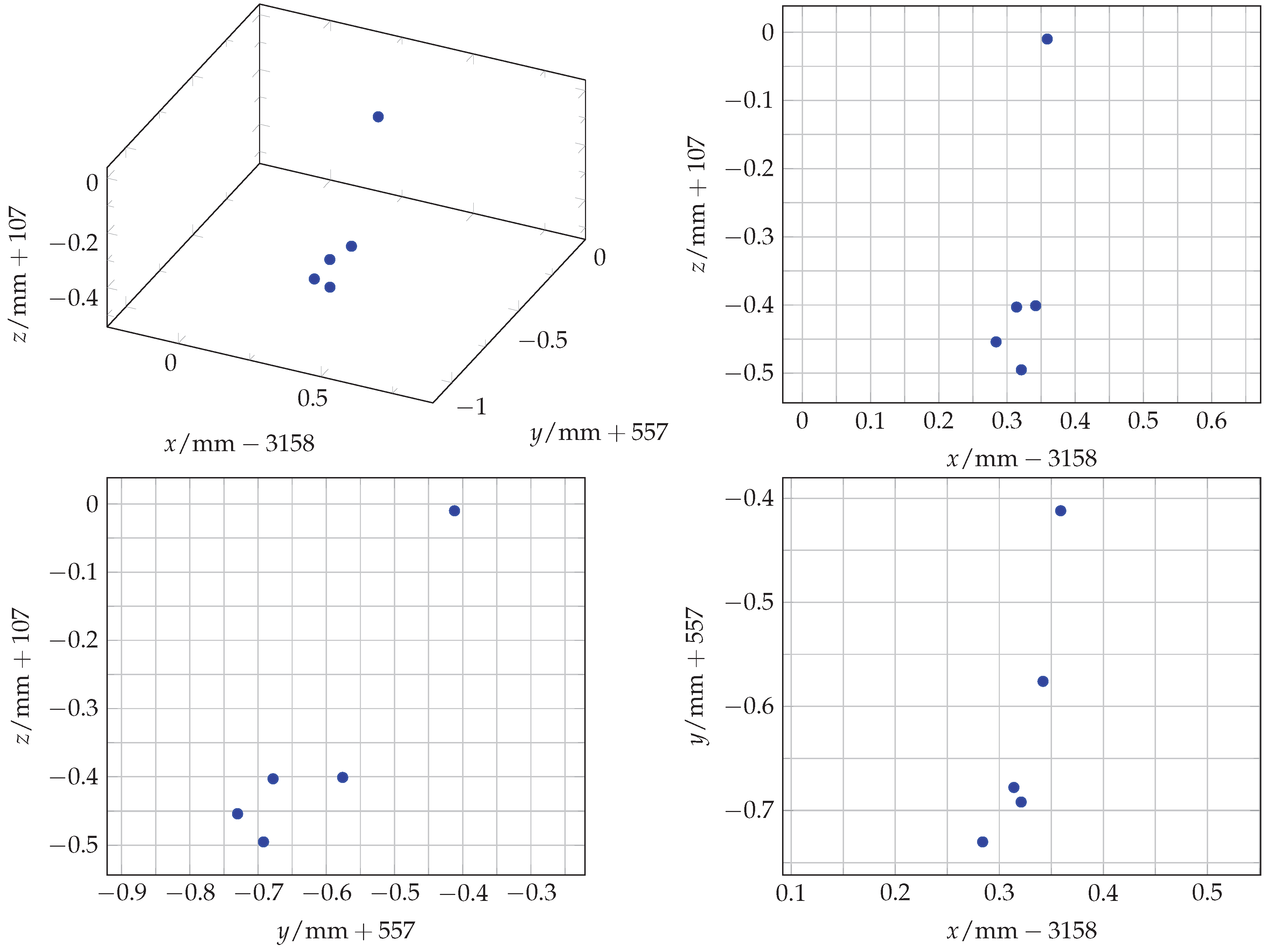

Table 1.
Analysed baseline measurement values for comparison and validation of the laboratory settings.
Table 1.
Analysed baseline measurement values for comparison and validation of the laboratory settings.
| x/mm | y/mm | z/mm | |
| Mean | 3158.43 | -556.389 | -107.327 |
| Median | 3158.43 | -556.39 | -107.327 |
| Min | 3158.428 | -556.413 | -107.331 |
| Max | 3158.436 | -556.365 | -107.321 |
| 0.008 | 0.048 | 0.01 | |
| Standard deviation | 3158.43(0.0018) | -556.389(0.0088) | -107.327(0.0021) |
Table 2.
Analysed radii of all ten eccentricity measurements.
| Measurement Run | Radius /mm |
| Circle 1_1 | 0.340 |
| Circle 1_2 | 0.315 |
| Circle 2_1 | 0.308 |
| Circle 2_2 | 0.324 |
| Circle 3_1 | 0.320 |
| Circle 3_2 | 0.317 |
| Circle 4_1 | 0.316 |
| Circle 4_2 | 0.321 |
| Circle 5_1 | 0.319 |
| Circle 5_2 | 0.353 |
Table 3.
Analysed repeatability measurement values of the SMR in monument placement.
| x/mm | y/mm | z/mm | |
| Mean | 3158.01 | -557.399 | -107.311 |
| Median | 3158 | -557.41 | -107.314 |
| Min | 3157.996 | -557.421 | -107.331 |
| Max | 3158.067 | -557.306 | -107.256 |
| 0.069 | 0.115 | 0.075 | |
| Standard deviation | 3158.01(0.02) | -557.399(0.0323) | -107.311(0.0199) |
Table 4.
Analysed repeatability measurement values of the mounting and dismounting of the mount.
| x/mm | y/mm | z/mm | |
| Mean | 3158.32 | -556.618 | -107.353 |
| Median | 3158.32 | -556.678 | -107.403 |
| Min | 3158.284 | -556.73 | -107.495 |
| Max | 3158.359 | -556.412 | -107.01 |
| 0.075 | 0.328 | 0.485 | |
| Standard deviation | 3158.32(0.0256) | -556.618(0.1147) | -107.353(0.1748) |
Table 5.
Comparison between the expected errors from the technical data sheet of the laser tracker FARO Vantage E and the Baseline Measurement (BaseM) values in the laboratory setting.
Table 5.
Comparison between the expected errors from the technical data sheet of the laser tracker FARO Vantage E and the Baseline Measurement (BaseM) values in the laboratory setting.
| Data sheet FARO Vantage E | BaseM | |
| mm | 0.018 | 0.008 |
| mm | 0.035 | 0.048 |
| mm | 0.035 | 0.01 |
Table 6.
Comparison between the Baseline Measurement (BaseM), the repeatability measurement of SMR in monument placement (RepM1) and the repeatability measurement of mounting and dismounting of the mount (RepM2)
Table 6.
Comparison between the Baseline Measurement (BaseM), the repeatability measurement of SMR in monument placement (RepM1) and the repeatability measurement of mounting and dismounting of the mount (RepM2)
| BaseM | RepM1 | RepM2 | |
| mm | 0.008 | 0.069 | 0.075 |
| mm | 0.048 | 0.115 | 0.328 |
| mm | 0.01 | 0.075 | 0.485 |
Table 7.
Display of microshifts of the robot during attachment of the mount by comparing an initial position and the positions after simulating fastening the screws.
Table 7.
Display of microshifts of the robot during attachment of the mount by comparing an initial position and the positions after simulating fastening the screws.
| x/mm | y/mm | z/mm | |
| Initial position | 3156.944 | -556.126 | -106.897 |
| Screw 1 | 3157.089 | -556.281 | -107.015 |
| Screw 2 | 3157.061 | -556.274 | -107.019 |
| Screw 3 | 3157.103 | -556.271 | -107.015 |
| Screw 4 | 3157.085 | -556.271 | -107.026 |
| Max. Shift | 0.159 | 0.155 | 0.129 |
| Position after 5 | 3156.869 | -556,256 | -106.995 |
| Position after 30 | 3156.943 | -556,140 | -106.901 |
Disclaimer/Publisher’s Note: The statements, opinions and data contained in all publications are solely those of the individual author(s) and contributor(s) and not of MDPI and/or the editor(s). MDPI and/or the editor(s) disclaim responsibility for any injury to people or property resulting from any ideas, methods, instructions or products referred to in the content. |
© 2024 by the authors. Licensee MDPI, Basel, Switzerland. This article is an open access article distributed under the terms and conditions of the Creative Commons Attribution (CC BY) license (http://creativecommons.org/licenses/by/4.0/mm).
Copyright: This open access article is published under a Creative Commons CC BY 4.0 license, which permit the free download, distribution, and reuse, provided that the author and preprint are cited in any reuse.


