
Submitted:
14 November 2024
Posted:
17 November 2024
You are already at the latest version
Abstract
Aquifer storage and recovery have gained attention as a solution that utilizes submarine groundwater discharge (SGD) as a surrogate water resource to alleviate water scarcity and fill the demand gap. Characterizing SGD is crucial for using coastal groundwater and improving understanding of the interaction between continental water and seawater. This study employs fiber-optical distributed temperature sensing (FODTS) and the heat tracer to quantify the groundwater flux in a coastal aquifer in northern Taiwan. The fluxes in different sections along the borehole were estimated from the temperature response caused by the active heating tests and campier groundwater flux under different tidal conditions, providing information on potential water resources for water resource planning and management. According to the active heating tests, the material of the sections with high-temperature response mainly consists of a gravel-sand mixture. Based on the estimations of groundwater fluxes along the well, the sections with low sensitivity of temperature response have low hydraulic conductivity and low groundwater flux. The estimated thermal parameters at the site are consistent with those obtained from the borehole samples in the laboratory tests. The groundwater fluxes in different sections are calculated based on the temperature response observed from the FODTS. The groundwater fluxes along the well vary between 0.02~1.77 m/day. There are considerable differences between the estimated fluxes during the tidal cycle in a heterogeneous coastal aquifer, indicating the high uncertainty of estimated SGD along coastal lines.
Keywords:
Submarine groundwater discharge
; fiber optic distributed temperature sensing
; active heating test
; coastal aquifer
; tidal
1. Introduction
Taiwan is a mountainous island with a particular climate and a diverse landscape. Due to the insufficient reservoir volume and steep slopes of mountains, storing precipitation as the primary water resource is challenging, even though the annual rainfall is about 2510 mm [1]. Other potential water resources should be considered and developed to fill the demand gap compared to conventional approaches, such as water conservation and recycling, to alleviate the problem of water scarcity. Considering groundwater as an offsetting option, the management approach is essential to ensure a sustainable water supply, prevent land subsidence and seawater intrusion in coastal areas, and preserve the ecosystem [2].
In recent years, the storage and recovery of water in aquifers have gained attention as a solution for meeting water demand; this approach has already been applied in many places [3,4,5]. Some cases in coastal areas have utilized submarine groundwater discharge as a substituted water resource and introduced the aquifer storage and recovery concept to manage it [6]. Submarine groundwater discharge (SGD), i.e., fresh groundwater discharge from the coastal aquifer to the sea, is essential in transporting pollutants and nutrients to the sea in coastal areas [7,8,9]. There are many cases where SGD is used as a water resource for domestic [10,11], agriculture [12,13], tourism [14,15,16] or religious practices [17]. Many studies have discussed the environmental factors that influence the amount of SGD, such as aquifer characteristics, coastal morphology, tidal conditions, waves, and sensory rainfall, which will determine the behavior of SGD in coastal areas [18,19,20,21,22,23,24]. Hence, the characterization and quantification of SGD are crucial for using freshwater discharge to the ocean. The results could also improve understanding of the interaction between continental water and seawater [25,26,27,28,29,30]. However, tidal fluctuations significantly influence the groundwater flow in the coastal area and increase the uncertainty of traditional pumping tests [31]. The detailed hydraulic properties of the aquifer are required to estimate groundwater flow in the coastal area.
Mismanagement of coastal groundwater practices, such as pumping, leads to subsidence, amplified by hydrogeological characteristics, and seawater intrusion results. To better manage the water resources and prevent environmental damage, the more we understand the groundwater system, the safer we can use the resource. Hence, many approaches have been developed to help the competent authority make decisions. Traditional hydraulic tests, such as pumping tests, are the most common approaches for determining hydraulic parameters. However, the results of these approaches are depth-averaged information and do not reveal layer characteristics that correctly analyze the spatial distribution of parameters along a well [34]. Many researchers attempt to estimate groundwater flux using different types of tracers, such as Jones et al. [35], who use isotope tracers to evaluate the relationship between surface runoff and groundwater discharge during rainfall events, and some researchers also use tracers to estimate groundwater velocity in shallow aquifer [36]. Moore et al. [37] used Radium-226 as an indicator to estimate the amount of SGD flowing into the sea.
Compared with other chemical tracers, the thermal tracer has many advantages, such as accessibility and low environmental impact. Heat is a natural groundwater tracer and can be measured in any aquifer. Most research uses the temperature difference between day and night to estimate groundwater flux, usually used in shallow aquifers or areas with high groundwater flux. Some researchers use heat as a tracer by releasing thermal energy that propagates with the flow to find the preferential flow path in the aquifer or fracture system [38]. The fiber-optical distributed temperature sensing (FODTS) system has been introduced in this field to collect temperature data along boreholes. FODTS has a high temporal-spatial resolution for measuring temperature along the fiber-optical cable [39,40], and many studies have shown the potential for analyzing groundwater flow and distribution characteristics [41]. Some studies have measured temperature variation induced by natural heat sources, while others have used artificial heat sources to create temperature differences [42,43,44,45]. Natural temperature fluctuations are more suitable for the characteristic behavior of large-scale groundwater flow, while artificial heating is more suitable for site-scale groundwater flow assessment. With the temperature profile of the borehole, the character of the layer could be revealed, and the flux could be estimated in a more detailed resolution.
In the study area, Dang et al. [46] collected hydraulic head measurements at a coastal site and developed a multi-phase groundwater model to assess the quantity of SGD using COMSOL Multi-physics software. From the numerical model, the average Darcy’s velocity in the study area was observed to be (2.96 ± 0.61) × 10-6 m/s, which is the same order of magnitude as the values reported for other sites in the world. The simulation results also show that the difference between high and low tidal conditions significantly influences Darcy’s velocity. However, the model was based on the homogeneous material assumption and used constant values for the hydrogeological parameters. Hence, an evaluation of coastal groundwater behavior based on field tests with information on the vertical direction is required.
This study aims to apply the heat tracer to quantify groundwater flux by deploying optical fiber in the observation wells with the FODTS system to collect high-resolution data and analyze the flux difference in different layers. FODTS enables us to perform high-resolution tracer tests and is easy to perform in various environments. Unlike the traditional test that gives an overall response along the entire borehole, the heat tracer with FODTS could provide detailed information (approximately every 25 cm with one observation) in the vertical direction. The groundwater fluxes in different sections of the borehole are then estimated from the temperature responses caused by the active heating tests. The estimated thermal parameters are compared with those measured from core samples in the laboratory. Moreover, the active heating tests under different tidal conditions provide temporal variations of groundwater fluxes along the well, and the groundwater fluxes at specific depths are estimated by fitting breakthrough curves obtained from the tests. The study uses heat tracer tests to characterize the site-specific surface water and seawater interactions under different tidal conditions and provide general insights into estimating potential water resources in a coastal aquifer.
2. Materials and Methods
2.1. Study Area
The study area is in northern Taiwan, as shown in Figure 1. We focused on the Taoyuan-Zhongli tablelands. The water supply in this area mainly depends on the Daham River upstream, and Shihmen Reservoir controls the inflow discharge to this area. According to the geological condition, two significant faults (Chuchih and Hsintien faults) with a strike from NE-SW have divided the study area into three geological provinces (I, II, and III). The study area is located in geological province III, the Taoyuan-Zhongli tablelands. It is the delta of the ancient Daham River, and the material is mainly composed of Pleistocene and Holocene young sediments. The rocks are mainly poorly cemented conglomerates and sequences of sandstones and mudstones. In the geological survey of the Taoyuan-Zhongli tablelands, the formation is only slightly folded, and the water infiltration is mainly dominated by the thin layer of lateritic terrace deposit (several meters to tens of meters). Therefore, the conceptual geological model of the study area follows the structure of the geological profile at the local scale and with site-specific core sampling data, as shown in Figure 2a. We assumed the geological model, as shown in Figure 2b, with the geology background based on the result of core drilling. The separation of the aquifer layers is based on the material types, including gravel-sand mixtures, gravelly sands, sand-silt mixtures, and sand-clay mixtures.
2.2. The Well Field, Experimental Setup, and Test Cases
The study area is located near the coastline, as shown in Figure 3a, and the configuration of the well field is shown in Figure 3b. The groundwater level and temperature of the study area are shown in Figure 3c, and the background water level and temperature have shown the influence of tidal conditions on the groundwater level fluctuation. The geological structure of the study site is assumed to be a typical layered structure based on the evolution process of the study area. This study applied an artificial heat source to the observation well to understand the geo-hydraulic characteristics of the aquifer and to capture the vertical distribution of groundwater flux under different tidal conditions in the study area. The main concept of the active heating test is to use the groundwater temperature deviating from the analytical solution without the influence of groundwater flow to estimate groundwater flux. The field configuration of the active heating test is shown in Figure 3d. The depth of the heating well BW02 is 50 m, and the diameter of the well is 4 inches. During the experiment, the well was heated by a line source, and the temperature variation was recorded simultaneously over time. The artificial heat source is a Teflon heater with a variable-frequency drive powered by a 220 Voltage power supply to control the temperature.
A FODTS system was used to measure the temperature in the borehole. The fiber-optical cable is installed in the borehole with the heater and passes through the cap and cold calibration baths. The measurement locations were identified by cooling spread to indicate the actual section in the borehole. The specifications of the OFDTS system can measure the temperature along the fiber-optic cable, as shown in Table 1. The FODTS is used to collect temperature data with higher resolution in space and time. The temperature data is calibrated using warm and cold baths, with the temperature measured by the PT 100.
The active heating approach is applied in a site-scale well field to improve the understanding of the geo-hydrological background in the study area. The temperature data will first identify materials through heat accumulation at different locations and estimate the groundwater flux by fitting analytical solutions. Each case represents different tidal conditions, as shown in Figure 4. Table 2 lists the detailed conditions for the heating tests.
In the study, Case 1 tests the temperature response of the borehole under different constant heating powers, with three heating powers tested to ensure that the temperature rise is appropriate. Cases 2 and 3 aim to quantify the behavior under two transitional tidal change situations. Case 2 is during the falling limb of the tidal cycle, Case 3 is during the rising limb of the tidal cycle, and these two cases are heated up for 4 hours and cooled for 9 hours. Cases 4 and 5 are designed to show the influence of changes in tidal conditions during the heating test. Both cases are heated up for 12.5 hours and cooled for 12 hours with opposite tidal changes.
2.3. Thermal Properties of Materials
The thermal properties measured on the core samples along the borehole are used to anchor the estimation as the initial value in the optimal process. In the study, the thermal conductivity of the materials was measured based on the transient line heat course method. In particular, the dual-needle method was used to measure the thermal properties, which was carried out using a thermal properties analyzer. Split needles with a heater and a temperature sensor were used during the measurement process. The heat was applied to the heating needle for a fixed heating time, and the temperature was measured from the other needle at a certain distance. The temperature of the sample was recorded during the heating and cooling and processed by subtracting the ambient temperature and the drift rate. The data obtained using the dual-needle method need to be fitted to Eqs. (1) and (2) based on the least-squares algorithm.
where ΔT is the temperature difference, q(W/m) is the thermal energy injected into the sample, k is thermal conductivity, r is the distance between two needles, D is the thermal diffusely, t is time, and th is the heating time. Table 3 lists the specifications of the thermal meter sensor for measuring the thermal properties in the study.
2.4. Mathematical Formulation of Groundwater Flux Estimation
Many researchers have focused on estimating groundwater flow by using the temperature response of the well [47,48]. Based on the previous studies, we applied the line-source heating of the borehole to estimate vertical groundwater flux, which one-dimensional heat and fluid transport function in a saturated aquifer [49] as follows:
where [W/m℃] is the thermal conductivity of the rock; T [℃] is the temperature; q [m/s] is the velocity of fluid passing through the aquifer; Cw and Cs [J/m3 ℃] are the volumetric heat capacity of fluid and rock, respectively, z [m] is the depth; T [s] is the time. Kipp [50] expands the function into the advection-dispersion function of heat transfer and the fluid transport function. The net energy change in a control volume is the sum of conduction, convection, dispersion, and heat source and sink and can be written as follows:
where is the water content [%], is the porosity[-], is the thermomechanical dispersion tensor [m2/s], is the specific discharge [m/s], is the source and sink term [m3], Ts is the temperature of source and sink [℃]. The left-hand side is the thermal energy change with time in a unit volume, the first term on the right-hand side is the conductive thermal transfer, the second is the dispersive thermal transfer, and the third is the advection thermal transfer. The last term is the source and sink.
In recent years, much research has been conducted on line-source heating tests to evaluate groundwater flow and the preferential flow path [51,52]. The main heat transfer mechanisms in the aquifer are heat convection and conduction in both vertical and horizontal directions. In an interlayer aquifer with an infinity length in the horizontal direction, the fluid can only be transported in a particular layer, the vertical exchange of fluid between layers is neglected, the material is uniform, and the influence of viscosity and density is also neglected, and assuming that the temperature between solid and fluid reaches equilibrium immediately. The temporal and spatial variation of the temperature in the aquifer can be written as follows:
where D [m2/s] is the heat diffusion coefficient, and is the heat retardation coefficient, which is related to the solid and fluid properties and can be expressed as follow:
where notation c [J/m3 K] is the buck thermal capacity of the aquifer, [kg/m3] is the buck density of the aquifer, and represents the mean fluid. Assume an infinitely long line source with constant heating power P [w/m], perpendicular to the groundwater flow, and the start point in the center of the coordinate system [53,54]. To reduce the uncertainty due to the distance between the heat source and the measurement location, the distribution of thermal conductivity, and the non-uniform groundwater flow, some studies rewrite the dimensionless functions based on the equations mentioned above as follows [55,56]:
where Dx [m2/s] and Dy [m2/s] are the heat diffusion coefficients in different directions, the equation is then converted into the analytical solution for the temperature variation under steady and uniform flow [57,58], which can be expressed as follows:
According to the temperature at steady state , the equation could be rewritten as follows:
Hence, assuming that the heat source is applied at t=0 and stops at t = t0, the temperature variation can be described as follows:
where the temperature change is related to parameter A, r/B, T(t∞), and the function of parameters such as q, , , , , and k. The groundwater flux in the x-direction (i.e., the horizontal direction) can be written as follows:
where q[m/s] is the flux in the x- direction, , and [J/(m3·K)] are the volumetric heat capacity of saturated soil and fluid, respectively, r is the distance between the heat source and the fiber-optical cable, [℃] is the thermal disparity in x-direction, and k[w/mK] is the effective thermal conductivity.
3. Results and Discussion
3.1. Characteristics of the Heat Transfer in the Borehole Subsections
The study defines a temperature response as the temperature increase from the background groundwater temperature during a heating process. The temperature response of Case 1 was compared with the background temperature variation in BW03 to confirm that the heating power is sufficient to produce a temperature difference compared to the background temperature change, which is around 1 ℃. The temperature profile of the BW02 heating borehole is shown in Figure 5. The BW02 well is a fully opened screen well except for the well casings installed in the top and bottom sections. The power of 4.8 kW overheated the borehole and reduced the power to 2.2 kW. During the 2.2kW power output, the temperature of the borehole continued to drop, and the power decreased to 3.5 kW. The temperature of the comparison point at 17 m was 3 ℃, which is higher than the background temperature change of 1 ℃. Therefore, a 3.5 Kw heating source was selected as the heating power for the rest of the tests in the study.
Under three different power supplies, Figure 5 shows clear temperature responses for different materials along the borehole. The casing sections near the top and bottom of the well show extremely high-temperature zones during the tests. The groundwater might not enter these zones. In general, layered materials in a well with low permeability or groundwater fluxes tend to accumulate heat faster and keep the temperature longer because of the relatively slow mixing of low groundwater inflow. In contrast, the highly permeable materials or fluxes surrounding the well allow more groundwater to pass the well. The heating process in the sections with highly permeable materials and groundwater fluxes could be slow and dissipate relatively fast. If the groundwater flow condition is similar, such behavior is an important indicator for identifying the permeability of the materials along a well and could be the information to validate the borehole samples from the drilling. In BW02, more substantial groundwater fluxes were observed near the interfaces for different material types. The section near 17m shows an example of this behavior. With the strong support of groundwater for the specific section, the same heating power will result in a relatively small variation of temperature increase during the tests.
The high groundwater flux layer might be the confined layer that provides additional pressure in the well. The groundwater in the well could flow upward or downward from the confined layer and push the temperature mixing zones upward or downward. It is critical to obtain the flow condition to determine the permeability of the material surrounding the well. In the study, we conducted packer tests that sealed the fully opened screen well in different sections and measured the water levels based on the sealed intervals. The tests confirmed a confining layer near 17m and one layer below 37m of the well. Specifically, the water levels from the layers near 17m and below 37m show the behavior of artesian wells, indicating that the pressurized groundwater flow might control the high groundwater fluxes in these two intervals.
Figure 6 shows the temperature variations during the heating and cooling processes applied to different cases. In Cases 2 and 3, the temperature response can determine the thermal dynamic characteristic of the heating well. The behaviors of different sections in the two cases are similar and can be divided into four specific sections, namely 6~17 m, 17~27 m, 27~37 m, and 37~47m. The top zone includes the well sections above the groundwater table and the casing above the depth of 6m. The bottom zone below 47m is also the casing zone for collecting sediment in the well. The data in these zones were not considered in the analyses because there was no groundwater interaction in these zones, and there was heat accumulation (see Figure 6).
In general, the temperature rise of section 17~27 m is relatively high, and the temperature rises by 3~4.8 ℃ because the materials in this section are gravel-sand mixtures and sandy silt layer with relatively low hydraulic conductivity or groundwater fluxes. The temperature response of section 27~37m is moderate, and materials in this section are gravel sand and a sand-clay mixture layer bound to the bottom. Sections near 15-17 m and 37~47 m are the relatively low-temperature response sections, in which the temperature increased by about 1~2 ℃. The materials of these two sections are gravelly sands and sand-silt mixtures with high groundwater fluxes, resulting in a non-significant temperature response. The patterns of temperature responses in the borehole are similar in Cases 4 and 5, in which the heating period includes high and low tide conditions. Still, a temperature drop can be observed in certain areas due to the change in downstream boundary conditions.
In some cases, heat accumulation occurs at a certain point due to the fiber-optical cable being in contact with the heating cable. We can summarize the overall temperature response characteristics by excluding those measurement points. Three types of temperature response sections can be distinguished based on the temperature variations in four cases: intense (or low groundwater flux), medium (moderate groundwater flux), and weak (high groundwater flux) impacts on the heating processes.
Notably, some locations show constant high-temperature responses in Cases 2, 3, and 4 and are inconsistent with the response of the adjacent measurement points. Such inconsistency might have been caused by the heating cable attached to the fiber-optic cable in the well. This behavior was not observed in Case 5 because the measurement uses the fiber-optic cable installed outside the well casing. Based on the results of the comparison between Case 5 and other cases, the patterns of temperature response sections are consistent except for the sections where the heating and fiber-optic cables are too close along the well.
Moreover, when the heating period is sustained over a complete tidal period, the groundwater flux increases during the heating period and the temperature decreases simultaneously—the groundwater flux increases when the tidal elevation decreases. The advantage of high-resolution temperature sensing is that it enables monitoring temperature variations with detailed heat interaction dynamics in a well. Take Case 4 as an example to demonstrate the section between 17-27m. In Figure 7, the red solid line indicates the variations in groundwater level, which varied with the tidal elevation. The red dotted line shows the pattern of the temperature variations in the 17-27m section during the heating process. Comparing the temperature pattern and groundwater levels in section 17-27m shows that a decreasing water level could increase groundwater flux. The temperature variations in Figure 7 are the important tidal-induced dynamics that have not been reported in previous investigations. The maximal variation of the temperature could reach 1 ℃ on average.
3.2. Thermal Properties of Core Samples
The thermal properties should correspond to the natural conditions on site to improve the reliability of the estimations. This study measured the core samples taken from the drilling well. The material type of core samples is identified as shown in Figure 2a. The aquifer of the study area is a typical layered structure in which the near-surface part consists of a soil gravel layer. The intermediate layer consists of an impermeable layer. The layers can be subdivided by their materials into different classifications, such as gravel-sand mixtures, gravelly sands, sand-silt mixtures, and sand-clay mixtures.
The thermal properties were measured based on the core samples obtained from well BW11. Selecting the samples relies on the judgment that the samples could represent the specific material types and the corresponding thermal properties. Table 4 lists the results of measured thermal properties at different depths. In the laboratory tests, the soil samples were under saturated conditions, and took the averaged values for multiple tests applied to a sample. Table 4 shows that the thermal conductivity of the materials varied from 1.45 W/mK to 2.536 W/mK. This result will be compared with the estimated results obtained from the thermal tomography model.
3.3. Estimations of Groundwater Fluxes
The data on the temporal sequence of temperature fluctuations were measured during the field heating tests, which included the heating and cooling phases to calculate the distribution of groundwater fluxes in the vertical direction. The calculation of groundwater flux is based on fitting the breakthrough curves obtained from the data obtained at different depths.
Cases 2 and 3 are measured during half a tidal cycle, while Cases 4 and 5 are measured through a complete tidal cycle. In the study, The thermal parameters measured from the saturated core samples in the laboratory are considered as the initial values and substituted into the governing equation to calculate the groundwater flux at a particular point along the well. Cases 4 and 5 serve as examples at a depth of 21.1m. Figure 8 shows the curve-fitting results for Cases 4 and 5. Case 4 includes an entire tidal period, and notice that the temperature response of Cases 4 and 5 are considerably influenced by the tidal condition, which could lead to 0.45 and 0.4 residual standard deviations for the curve fitting. Such results show the limited feature of the current analytical solution, which does not consider the influence of the tidal variation. Therefore, the following discussion will focus on Cases 2 and 3. Figure 9 shows the fitting curves for Cases 2 and 3. As the figures show, the residuals and noise are consistent in both cases and lie between -0.5 and 0.5, which could be due to the systematic noise of the DTS system. The temperature increase is much higher than the noise. Therefore, this noise is neglected after the curve fitting processes.
Figure 10 shows the optimal fitted parameters for Cases 2 and 3. Compared with parameter A, parameter B shows a significant difference between Case 2 and Case 3. Results show that the groundwater flux in the two cases is different. Note that the distance between the heat source and the fiber-optical cable could be consistent because no adjustment is applied to the instrument in the well. The differences of parameters A and B in Cases 2 and 3 could represent the influences of tidal-induced groundwater flux change.
Figure 11 shows the result of the estimated horizontal groundwater flux along the well. For Cases 2 and 3, opposite tidal conditions are represented, i.e., from high tide to low tide conditions and from low tide to high tide conditions. In Case 2, the seaside boundary drops, and the hydraulic gradient between the ocean and land increases, forcing the groundwater flow out of the aquifer. In contrast, in Case 3, the opposite situation is obtained. The hydraulic gradient gradually decreases and constrains groundwater discharge to the sea. There are significant differences between coarse material and fine material sections. Parameter A is a lumped parameter that accounts for the behavior of the diffusion coefficients in different sections. However, parameter B combines the diffusion coefficient and flux effects in a specific section. Parameter B is proportional to the dispersion coefficient and inversely proportional to the flux. Cases 2 and 3 are the tidal cycle's falling and rising limbs. The variations of the parameter A along the well are relatively stable in the center sections. However, the sections near the well top and bottom show significant differences in the A values, which might be controlled by the heat diffusivity of materials. The variations of B in Cases 2 and 3 show significant differences below 17 m and above 37m. Parameter B is the coupled effects of the diffusion coefficient, the flux, and the ratio of aquifer volumetric heat capacity and fluid volumetric heat capacity. During the Cases 2 and 3 experiments, the aquifer and fluid volumetric heat capacity ratio might be similar. The characteristics of Dx/q could control the variations of B values (see Eq. (12)).
Compared the flux estimation with the material type and the temperature response during the heating tests, as Figure 12 and Figure 13 shows, the groundwater fluxes in Case 2 vary in the range of 1.77~0.2 m/day, and 0.25~0.02m/day for Case 3. The difference between these two tidal conditions could be more than an order of magnitude. The estimated average groundwater flux along the well in Case 2 is 0.5 m/day and is consistent with a previous study conducted at the site, which used a numerical model with observed hydraulic data from pumping tests [46]. Notably, the distribution of flux in the vertical direction is highly different and controlled by the layer materials. The tidal conditions highly influence the sections below 19 m, mainly covering the intense temperature response intervals. However, the section near 18m shows relatively small differences between Cases 2 and 3. There might be an intense flux near 18m. The tidal variations have less influence on flux calculation.
4. Conclusions
This study uses the fiber-optical cable and the DTS system to monitor the temperature variations in the borehole during heating tests under different tidal conditions. The high-resolution temperature data and thermal properties measured from core samples were used to calculate the temperature response and further estimate the groundwater fluxes along a well. Based on the results of the study, the FODTS system associated with field active heating tests can improve the efficiency of field experiments and provide information on groundwater fluxes under changing tidal conditions.
The study has defined a temperature response as the temperature increase from the background groundwater temperature during a heating process. According to the temperature variation along the heating well through the heating tests, the temperature response can be used to estimate the hydraulic conductivity in different sections along a fully open screen well. The active heating test revealed the thermal behavior along the borehole. The material of each section could be identified based on the heat responses in the heating and cooling processes. The depths 17-27 m and 27-37m are sections with high and moderate temperature responses. The sections with relatively low-temperature response are 6-17m and 37-47m. The groundwater flux estimation for these sections with low permeability and low groundwater flux is consistent with the results of the temperature response.
The groundwater flux is calculated according to the temperature response of each depth, and the range of groundwater flux is between 0.02 and 1.77 m/day. The heating period includes an entire tidal cycle that could influence the temperature response of tests. Based on the high-resolution temperature sensing technology, the study could map the detailed tidal-induced dynamics of temperature variations in a well. Comparing the temperature pattern and groundwater levels shows that a decreasing water level could increase groundwater flux. The maximal variation of the temperature reaches 1 ℃, indicating the connection between coastal aquifers and the ocean.
Author Contributions
Conceptualization, Yu-Huan Chang, Chuen-Fa Ni; methodology, Yu-Huan Chang, Chia-Yu Hsu; software, Chia-Yu Hsu, An-Yi Hsu; validation, Yu-Huan Chang, Chi-Ping Lin, Nguyen Hoang Hiep, Doan Thi Thanh Thuy; writing—original draft preparation, Yu-Huan Chang; writing—review and editing, Chuen-Fa Ni; visualization, Yu-Huan Chang, Chi-Ping Lin. All authors have read and agreed to the published version of the manuscript.”.
Funding
This research was partially supported by the National Science and Technology Council, Taiwan, under grants NSTC 111-2621-M-008-003, NSTC 112-MOEA-M-008-001, NSTC 112-2123-M-008-001, NSTC 112-2122-M-007-002 and NSTC 113-MOEA-M-008-001.
Data Availability Statement
N/A.
Acknowledgments
The authors thank the Taiwan Water Resource Agency (WRA) and Central Geological Survey (CGS) for the groundwater data, tidal data, hydrogeological loggings, and lithology data.
Conflicts of Interest
The authors declare no conflicts of interest.
References
- Wang, Shih-Jung, et al. Evaluation of climate change impact on groundwater recharge in groundwater regions in Taiwan. Water, 2021, 13.9, 1153. [CrossRef]
- Vengadesan, Manivannan; Lakshmanan, Elango. Management of coastal groundwater resources. In: Coastal Management. Academic Press, 2019, 383-397.
- Khan, Shahbaz, et al. Estimating potential costs and gains from an aquifer storage and recovery program in Australia. Agricultural water management, 2008, 95.4, 477-488. [CrossRef]
- Niazi, Amir, et al. A system dynamics model to conserve arid region water resources through aquifer storage and recovery in conjunction with a dam. Water, 2014, 6.8, 2300-2321.
- Lluria, Mario R.; Paski, Phillip M.; Small, Gary G. Seasonal water storage and replenishment of a fractured granitic aquifer using ASR wells. Sustainable Water Resources Management, 2018, 4, 261-274. [CrossRef]
- McCoy, C. A.; Corbett, D. R. Review of submarine groundwater discharge (SGD) in coastal zones of the Southeast and Gulf Coast regions of the United States with management implications. Journal of environmental management, 2009, 90.1, 644-651. [CrossRef]
- Bishop, James M., et al. Effect of land use and groundwater flow path on submarine groundwater discharge nutrient flux. Journal of Hydrology: Regional Studies, 2017, 11, 194-218. [CrossRef]
- Richardson, Christina M.; Dulai, Henrietta; Whittier, Robert B. Sources and spatial variability of groundwater-delivered nutrients in Maunalua Bay, Oʻahu, Hawai ‘i. Journal of Hydrology: Regional Studies, 2017, 11, 178-193. [CrossRef]
- Yu, Xuan; Michael, Holly A. Offshore pumping impacts onshore groundwater resources and land subsidence. Geophysical Research Letters, 2019, 46.5, 2553-2562. [CrossRef]
- Dimova, Natasha T.; Burnett, William C.; Speer, Kevin. A natural tracer investigation of the hydrological regime of Spring Creek Springs, the largest submarine spring system in Florida. Continental Shelf Research, 2011, 31.6, 731-738. [CrossRef]
- Gilli, Eric. Deep speleological salt contamination in Mediterranean karst aquifers: perspectives for water supply. Environmental Earth Sciences, 2015, 74, 101-113. [CrossRef]
- Milanovic, Petar. Water resources engineering in karst. CRC press, 2004.
- Pereira, L. S., et al. (ed.). Sustainability of irrigated agriculture, Springer Science & Business Media, 2013. [CrossRef]
- Burnett, Kimberly, et al. The economic value of groundwater in Obama. Journal of Hydrology: Regional Studies, 2017, 11, 44-52. [CrossRef]
- Hata, Masaki, et al. Occurrence, distribution and prey items of juvenile marbled sole Pseudopleuronectes yokohamae around a submarine groundwater seepage on a tidal flat in southwestern Japan. Journal of Sea Research, 2016, 111, 47-53. [CrossRef]
- Utsunomiya, Tatsuya, et al. Higher species richness and abundance of fish and benthic invertebrates around submarine groundwater discharge in Obama Bay, Japan. Journal of Hydrology: Regional Studies, 2017, 11, 139-146. [CrossRef]
- Moosdorf, Nils; Oehler, Till. Societal use of fresh submarine groundwater discharge: An overlooked water resource. Earth-Science Reviews, 2017, 171, 338-348. [CrossRef]
- Smith, Anthony J. Mixed convection and density-dependent seawater circulation in coastal aquifers. Water Resources Research, 2004, 40.8. [CrossRef]
- Kaleris, Vassilios. Submarine groundwater discharge: Effects of hydrogeology and of near shore surface water bodies. Journal of Hydrology, 2006, 325.1-4, 96-117. [CrossRef]
- Konikow, Leonard F., et al. Seawater circulation in sediments driven by interactions between seabed topography and fluid density. Water Resources Research, 2013, 49.3, 1386-1399. [CrossRef]
- Uchiyama, Yusuke, et al. Submarine groundwater discharge into the sea and associated nutrient transport in a sandy beach. Water Resources Research, 2000, 36.6, 1467-1479. [CrossRef]
- Kohout, F. A. A hypothesis concerning cyclic flow of salt water related to geothermal heating in the Floridan aquifer. Transactions of the New York Academy of Sciences, 1965, 28.2, 249-271.
- Longuet-Higgins, Michael Selwyn. Wave set-up, percolation and undertow in the surf zone. Proceedings of the Royal Society of London. A. Mathematical and Physical Sciences, 1983, 390.1799, 283-291.
- Anderson Jr, William P.; Emanuel, Ryan E. Effect of interannual climate oscillations on rates of submarine groundwater discharge. Water Resources Research, 2010, 46.5.
- Cable, Jaye E.; Martin, Jonathan B. In situ evaluation of nearshore marine and fresh pore water transport into Flamengo Bay, Brazil. Estuarine, Coastal and Shelf Science, 2008, 76.3, 473-483. [CrossRef]
- Martin, Jonathan B., et al. Magnitudes of submarine groundwater discharge from marine and terrestrial sources: Indian River Lagoon, Florida. Water Resources Research, 2007, 43.5. [CrossRef]
- McCoy, C. A., et al. Hydrogeological characterization of southeast coastal plain aquifers and groundwater discharge to Onslow Bay, North Carolina (USA). Journal of Hydrology, 2007, 339.3-4, 159-171. [CrossRef]
- Thompson, Craig; Smith, Leslie; Maji, Roudrajit. Hydrogeological modeling of submarine groundwater discharge on the continental shelf of Louisiana. Journal of Geophysical Research: Oceans, 2007, 112.C3. [CrossRef]
- Wilson, Alicia M. Fresh and saline groundwater discharge to the ocean: A regional perspective. Water Resources Research, 2005, 41.2. [CrossRef]
- Burnett, W. C., et al. Quantifying submarine groundwater discharge in the coastal zone via multiple methods. Science of the total Environment, 2006, 367.2-3, 498-543. [CrossRef]
- Chapuis, Robert P.; Bélanger, Christian; Chenaf, Djaouida. Pumping test in a confined aquifer under tidal influence. Groundwater, 2006, 44.2, 300-305. [CrossRef]
- Jim Yeh, T.-C. Stochastic modelling of groundwater flow and solute transport in aquifers. Hydrological Processes, 1992, 6.4, 369-395. [CrossRef]
- Yeh, T.-C. Jim. Scale issues of heterogeneity in vadose zone hydrology and practical solutions, Department of Hydrology and Water Resources, University of Arizona (Tucson, AZ), 1996.
- Lin C.P., Chang Y.H., Ni C.F. Constructing and evaluating cross-borehole heat tracer tests to analyze the local-scale aquifer flow characteristics. Journal of Soil and Groundwater Remediation, 2022, 7(2), 81-112.
- Jones, J. P., et al. An assessment of the tracer-based approach to quantifying groundwater contributions to streamflow. Water Resources Research, 2006, 42.2. [CrossRef]
- Reilly, Thomas E., et al. The use of simulation and multiple environmental tracers to quantify groundwater flow in a shallow aquifer. Water Resources Research, 1994, 30.2, 421-433. [CrossRef]
- Moore, Willard S. Large groundwater inputs to coastal waters revealed by 226Ra enrichments. Nature, 1996, 380.6575, 612-614. [CrossRef]
- Pehme, P. E., et al. Enhanced detection of hydraulically active fractures by temperature profiling in lined heated bedrock boreholes. Journal of Hydrology, 2013, 484: 1-15. [CrossRef]
- Ukil, Abhisek; Braendle, Hubert; Krippner, Peter. Distributed temperature sensing: Review of technology and applications. IEEE Sensors Journal, 2011, 12.5, 885-892. [CrossRef]
- Van de Giesen, Nick, et al. Double-ended calibration of fiber-optic Raman spectra distributed temperature sensing data. Sensors, 2012, 12.5, 5471-5485.
- Selker, Frank; Selker, John S. Investigating water movement within and near wells using active point heating and fiber optic distributed temperature sensing. Sensors, 2018, 18.4, 1023. [CrossRef]
- Banks, Eddie W.; Shanafield, Margaret A.; Cook, Peter G. Induced temperature gradients to examine groundwater flowpaths in open boreholes. Groundwater, 2014, 52.6, 943-951. [CrossRef]
- Leaf, Andrew T.; Hart, David J.; Bahr, Jean M. Active thermal tracer tests for improved hydrostratigraphic characterization. Groundwater, 2012, 50.5, 726-735. [CrossRef]
- Liu, G.; Knobbe, S.; Butler Jr, J. J. Resolving centimeter-scale flows in aquifers and their hydrostratigraphic controls. Geophysical Research Letters, 2013, 40.6, 1098-1103.
- Anderson, Mary P. Heat as a ground water tracer. Groundwater 2005, 43.6, 951-968. [CrossRef]
- Dang, Minh-Quan, et al. Coastal flowing artesian wells and submarine groundwater discharge driven by tidal variation at TaiCOAST site in Taoyuan, Taiwan. Journal of Hydrology: Regional Studies, 2024, 52, 101708. [CrossRef]
- Reiter, Marshall. Using precision temperature logs to estimate horizontal and vertical groundwater flow components. Water Resources Research, 2001, 37.3, 663-674. [CrossRef]
- Drury, M. J.; Jessop, A. M.; Lewis, T. J. The detection of groundwater flow by precise temperature measurements in boreholes. Geothermics, 1984, 13.3, 163-174. [CrossRef]
- Stallman, R. W. Steady one-dimensional fluid flow in a semi-infinite porous medium with sinusoidal surface temperature. Journal of geophysical Research, 1965, 70.12, 2821-2827. [CrossRef]
- Kipp, Kenneth L. HST3D: A computer code for simulation of heat and solute transport in three-dimensional ground-water flow systems, US Geological Survey, 1987.
- Bakker, Mark, et al. An active heat tracer experiment to determine groundwater velocities using fiber optic cables installed with direct push equipment. Water Resources Research, 2015, 51.4, 2760-2772. [CrossRef]
- des Tombe, Bas F., et al. Estimation of the variation in specific discharge over large depth using distributed temperature sensing (DTS) measurements of the heat pulse response. Water Resources Research, 2019, 55.1, 811-826.
- Kluitenberg, G. J.; Warrick, A. W. Improved evaluation procedure for heat-pulse soil water flux density method. Soil Science Society of America Journal, 2001, 65.2, 320-323. [CrossRef]
- Ren, T.; Kluitenberg, G. J.; Horton, R. Determining soil water flux and pore water velocity by a heat pulse technique. Soil Science Society of America Journal, 2000, 64.2, 552-560. [CrossRef]
- Hopmans, Jan W.; Šimunek, Jirka; Bristow, Keith L. Indirect estimation of soil thermal properties and water flux using heat pulse probe measurements: Geometry and dispersion effects. Water Resources Research, 2002, 38.1, 7-1-7-14. [CrossRef]
- Smith, Leslie; Chapman, David S. On the thermal effects of groundwater flow: 1. Regional scale systems. Journal of Geophysical Research: Solid Earth, 1983, 88.B1, 593-608. [CrossRef]
- Zubair, S. M.; Chaudhry, M. Aslam. Temperature solutions due to time-dependent moving-line-heat sources. Heat and Mass Transfer, 1996, 31.3, 185-189.
- Diao, Nairen; LI, Qinyun; Fang, Zhaohong. Heat transfer in ground heat exchangers with groundwater advection. International Journal of Thermal Sciences, 2004, 43.12, 1203-1211. [CrossRef]
Figure 1.
The geological map of the study area is divided into (I) the western Hsuehshan Range belt, (II) the western foothills province, and (III) the Taoyuan-Zhongli tablelands.
Figure 1.
The geological map of the study area is divided into (I) the western Hsuehshan Range belt, (II) the western foothills province, and (III) the Taoyuan-Zhongli tablelands.
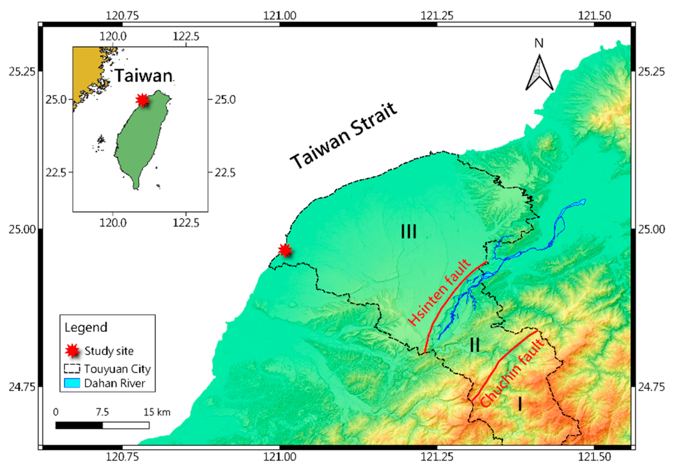
Figure 2.
The borehole data and the conceptual model of the coastal aquifer at the site: (a.) The material types of each layer were obtained from the core samples; (b) The conceptual model of the groundwater flow at the site was based on observations from the borehole drilling logs and previous investigations.
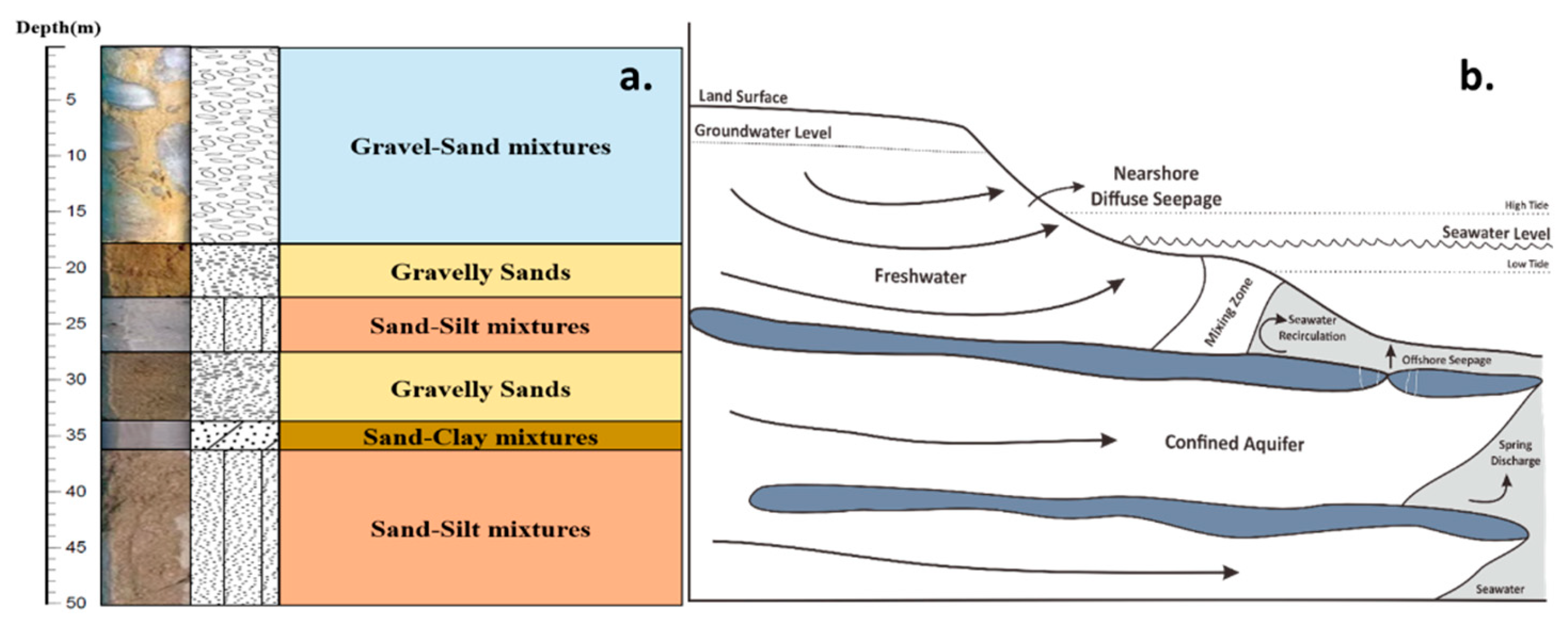
Figure 3.
The site-specific conditions and the facilities for the study site: (a.) The aerial shot of the study area near the coastal line; (b.) The configuration of the well field and the locations of well BW02; (c.) The background groundwater level and temperature measured in well BW01, and (d.) The field configuration of the active heating test setup.
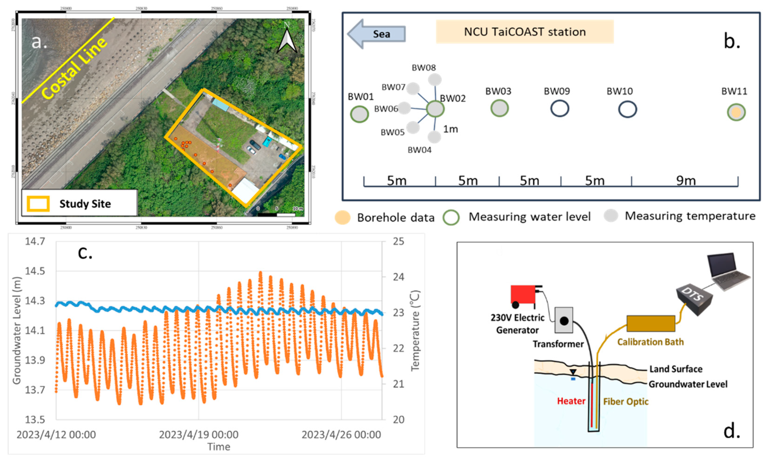
Figure 4.
The experimental periods for different cases as compared to the tidal variations. The red lines indicate the heating period, and the blue lines indicate the cooling periods during the active heating tests.
Figure 4.
The experimental periods for different cases as compared to the tidal variations. The red lines indicate the heating period, and the blue lines indicate the cooling periods during the active heating tests.
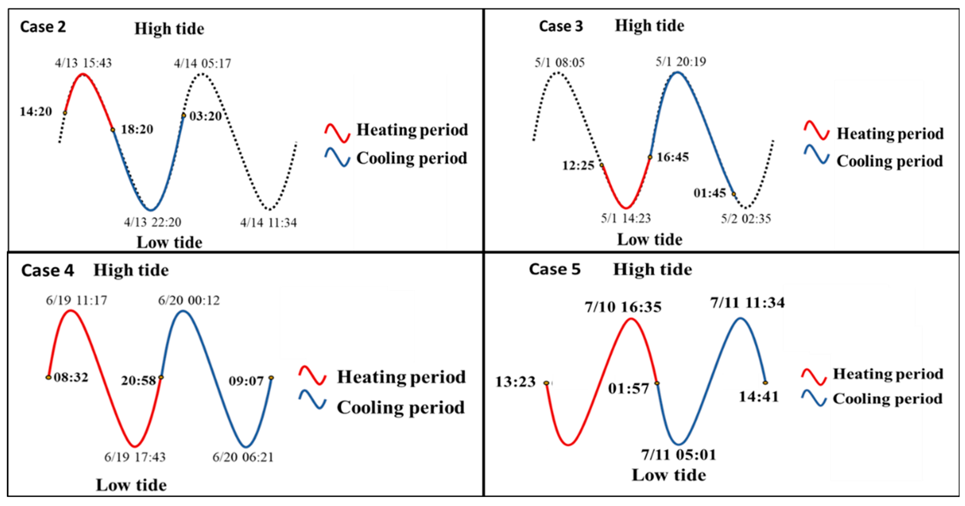
Figure 5.
The geological profile of BW02 obtained from the core samples and the temperature profile of BW02 during Case 1. The red dashed lines indicate the periods of different heating powers.
Figure 5.
The geological profile of BW02 obtained from the core samples and the temperature profile of BW02 during Case 1. The red dashed lines indicate the periods of different heating powers.
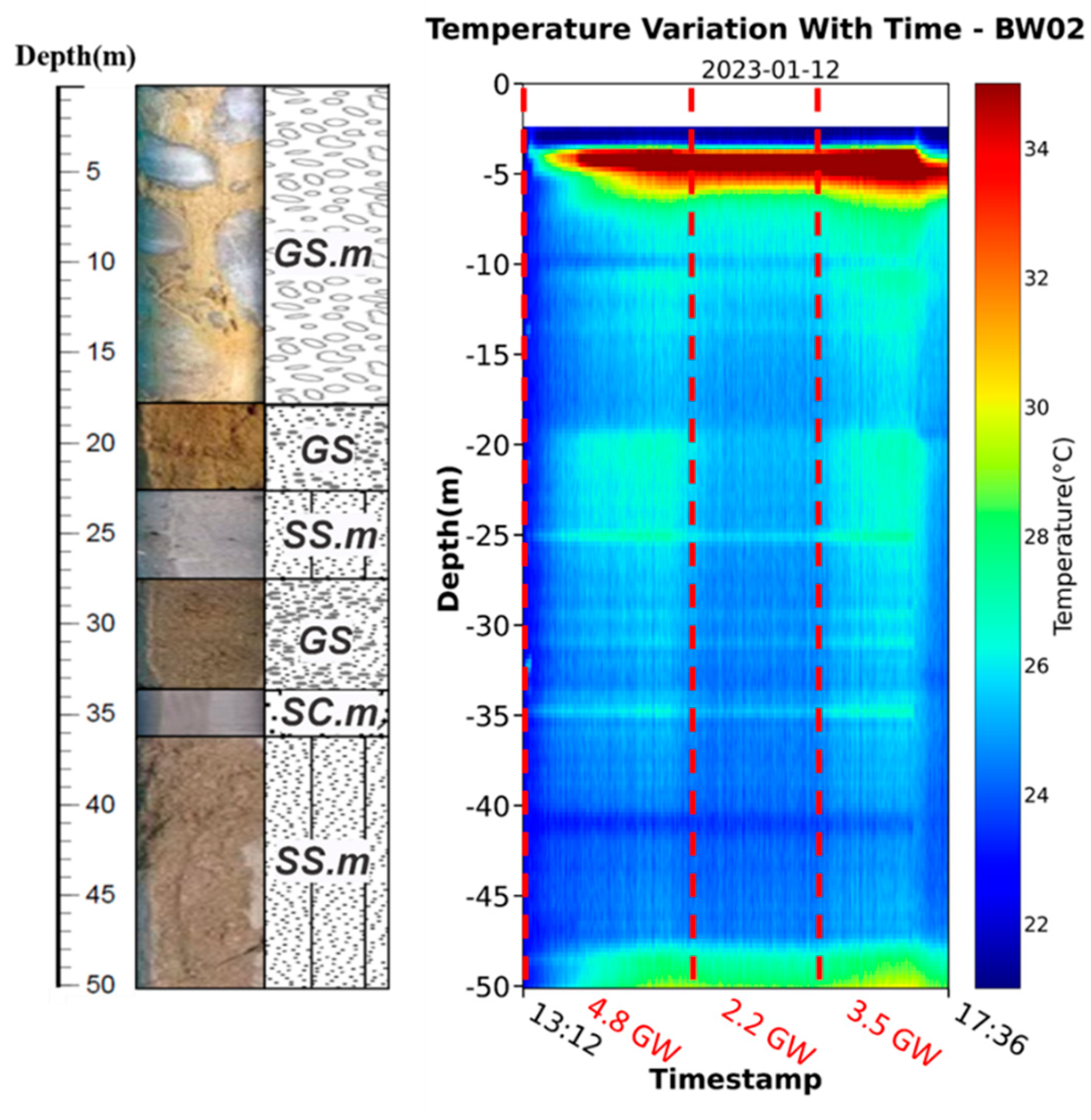
Figure 6.
The comparison of the results for four heating cases. The time duration of Case 2 and Case 3 is a half-tidal period, and Case 4 and Case 5 is a full-tidal period. The temperature variation with time shows the tidal condition influences groundwater flow with time. Prominent heat accumulation portions are in the well casing sections located on the top and bottom of the well.
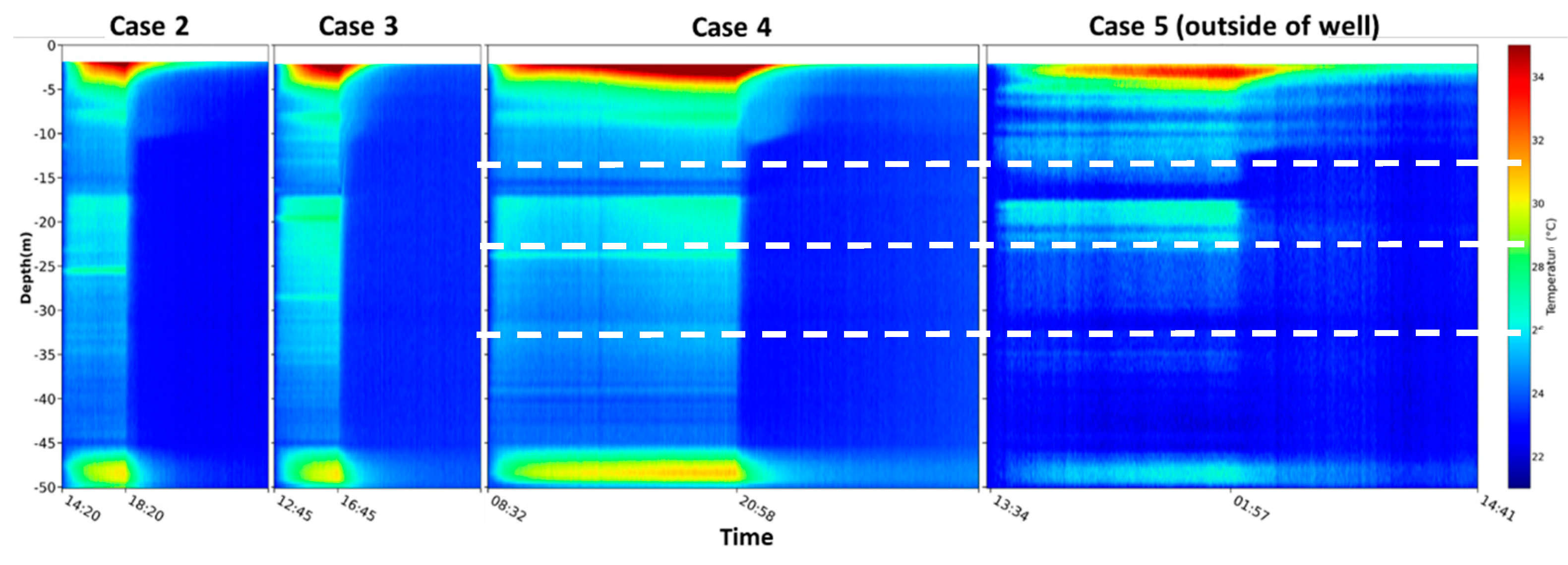
Figure 7.
The temperature and groundwater level variations of Case 4 under the tidal cycle condition. The increase and decrease of groundwater water levels simultaneously reflect the tidal variations because of the short distance from the well to the coastal line.
Figure 7.
The temperature and groundwater level variations of Case 4 under the tidal cycle condition. The increase and decrease of groundwater water levels simultaneously reflect the tidal variations because of the short distance from the well to the coastal line.
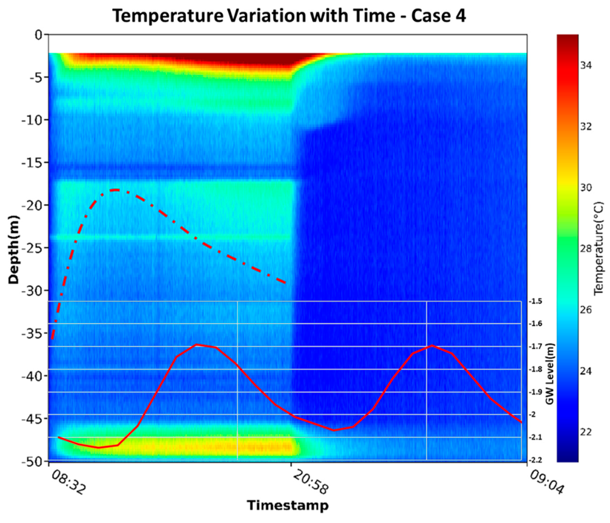
Figure 8.
Comparison between the estimated and measured temperature, the residuals, and the noise in Cases 4 and 5.
Figure 8.
Comparison between the estimated and measured temperature, the residuals, and the noise in Cases 4 and 5.
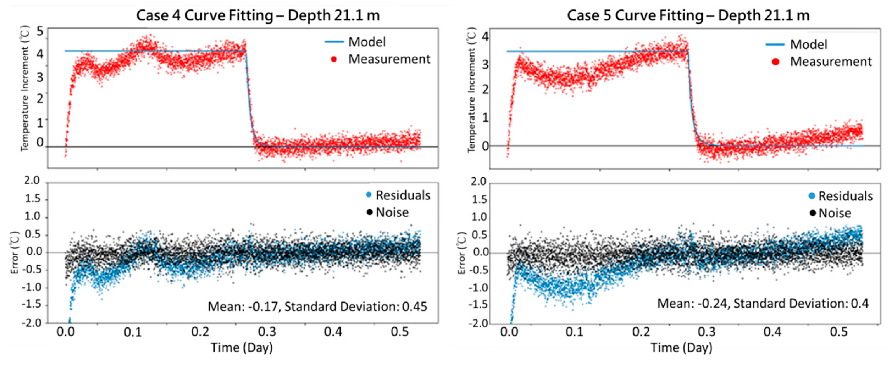
Figure 9.
Comparison between the estimated and measured temperature, the residuals, and the noise in Cases 2 and 3.
Figure 9.
Comparison between the estimated and measured temperature, the residuals, and the noise in Cases 2 and 3.
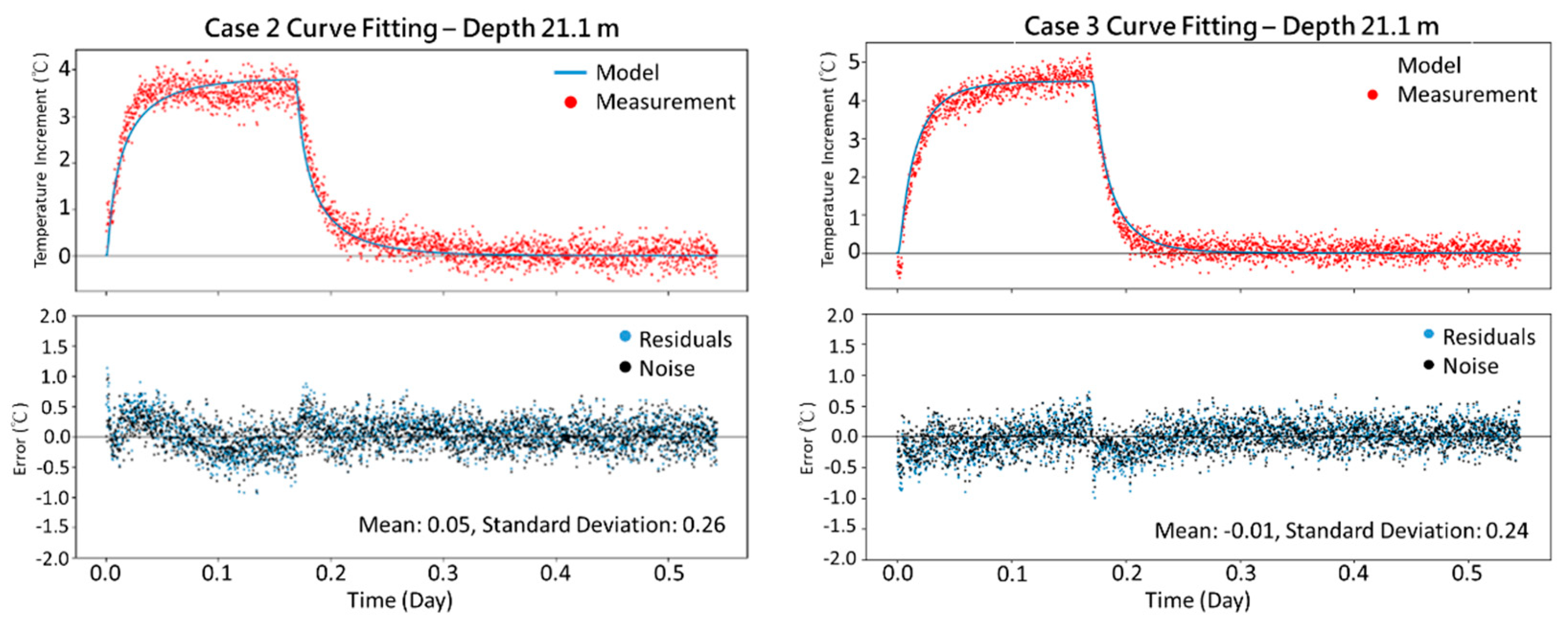
Figure 10.
Fitting parameters A and B for estimating groundwater fluxes along the observation well. The black and red lines are the groundwater flux of Cases 2 and 3, respectively.
Figure 10.
Fitting parameters A and B for estimating groundwater fluxes along the observation well. The black and red lines are the groundwater flux of Cases 2 and 3, respectively.
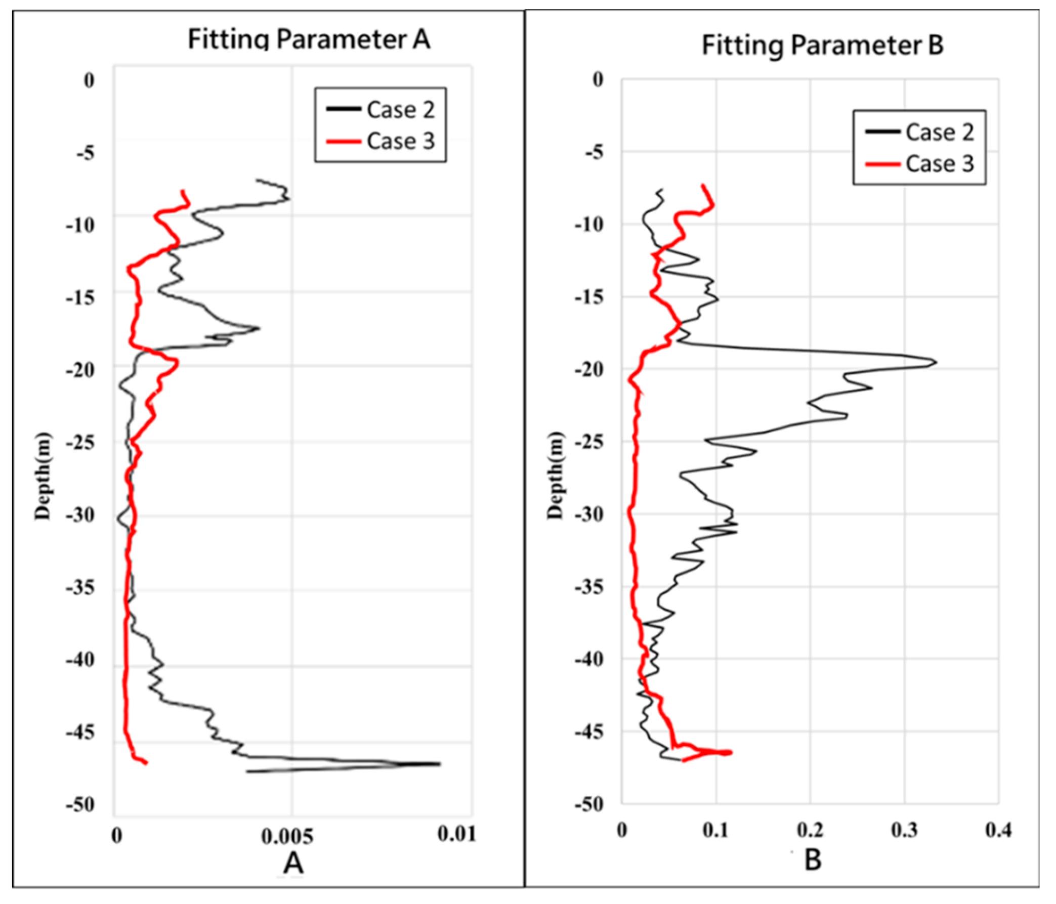
Figure 11.
Estimation of the groundwater fluxes of BW02 under different tidal conditions. The black and green lines are the groundwater flux of Cases 2 and 3, respectively.
Figure 11.
Estimation of the groundwater fluxes of BW02 under different tidal conditions. The black and green lines are the groundwater flux of Cases 2 and 3, respectively.
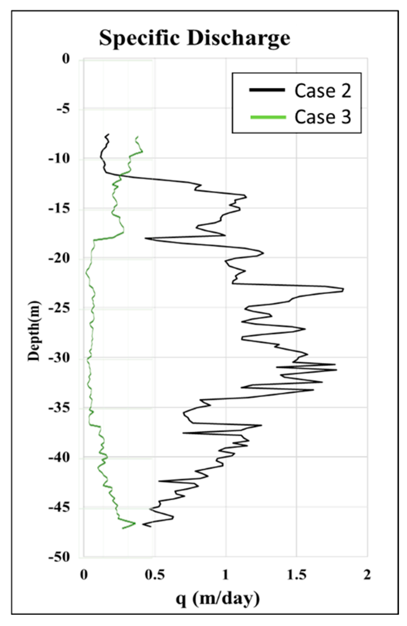
Figure 12.
The comparison between the geological logging, the temperature response, and the estimated groundwater flux from Case 2.
Figure 12.
The comparison between the geological logging, the temperature response, and the estimated groundwater flux from Case 2.
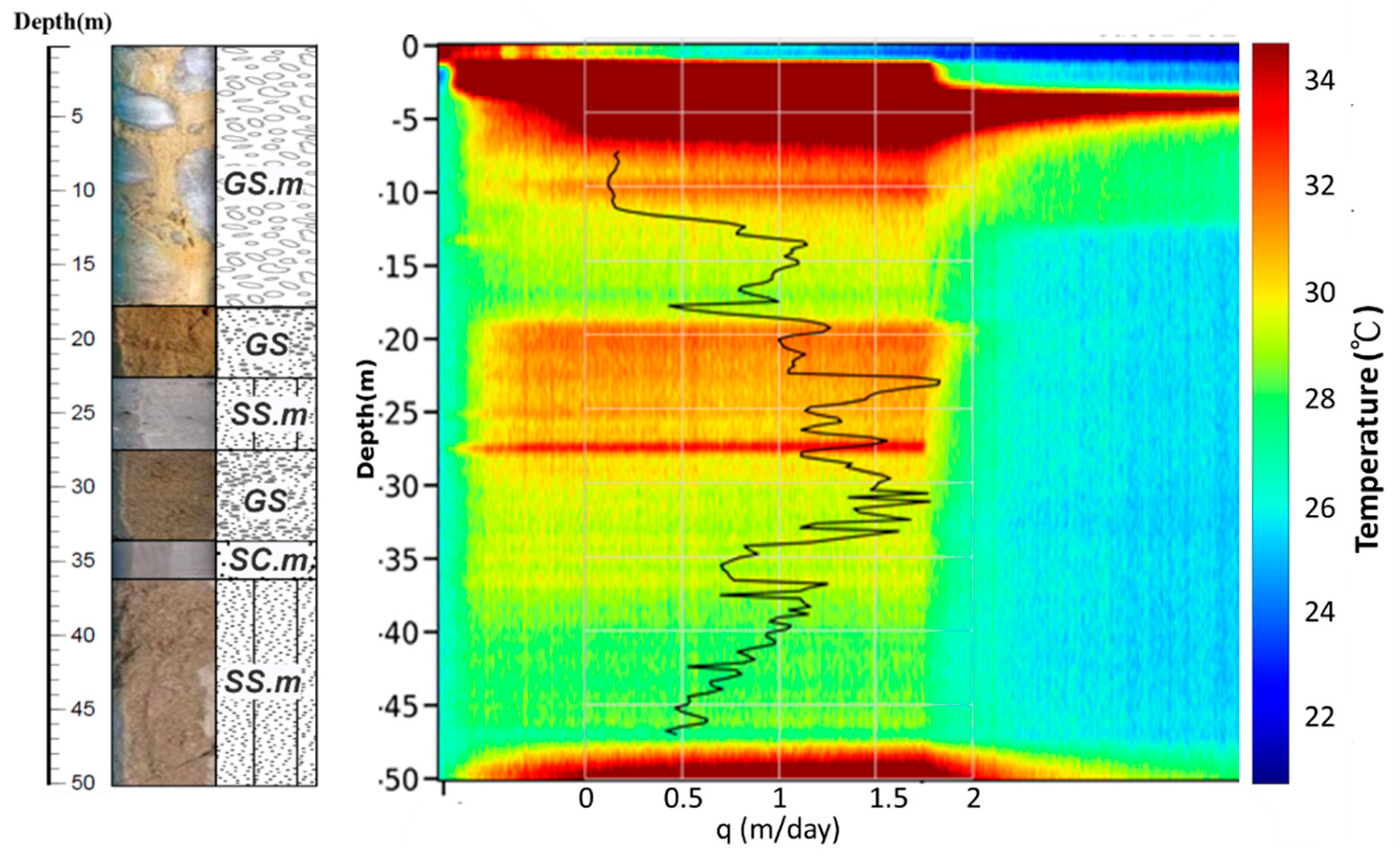
Figure 13.
The comparison between the geological loggings, the temperature response, and the estimated groundwater flux from Case 3.
Figure 13.
The comparison between the geological loggings, the temperature response, and the estimated groundwater flux from Case 3.
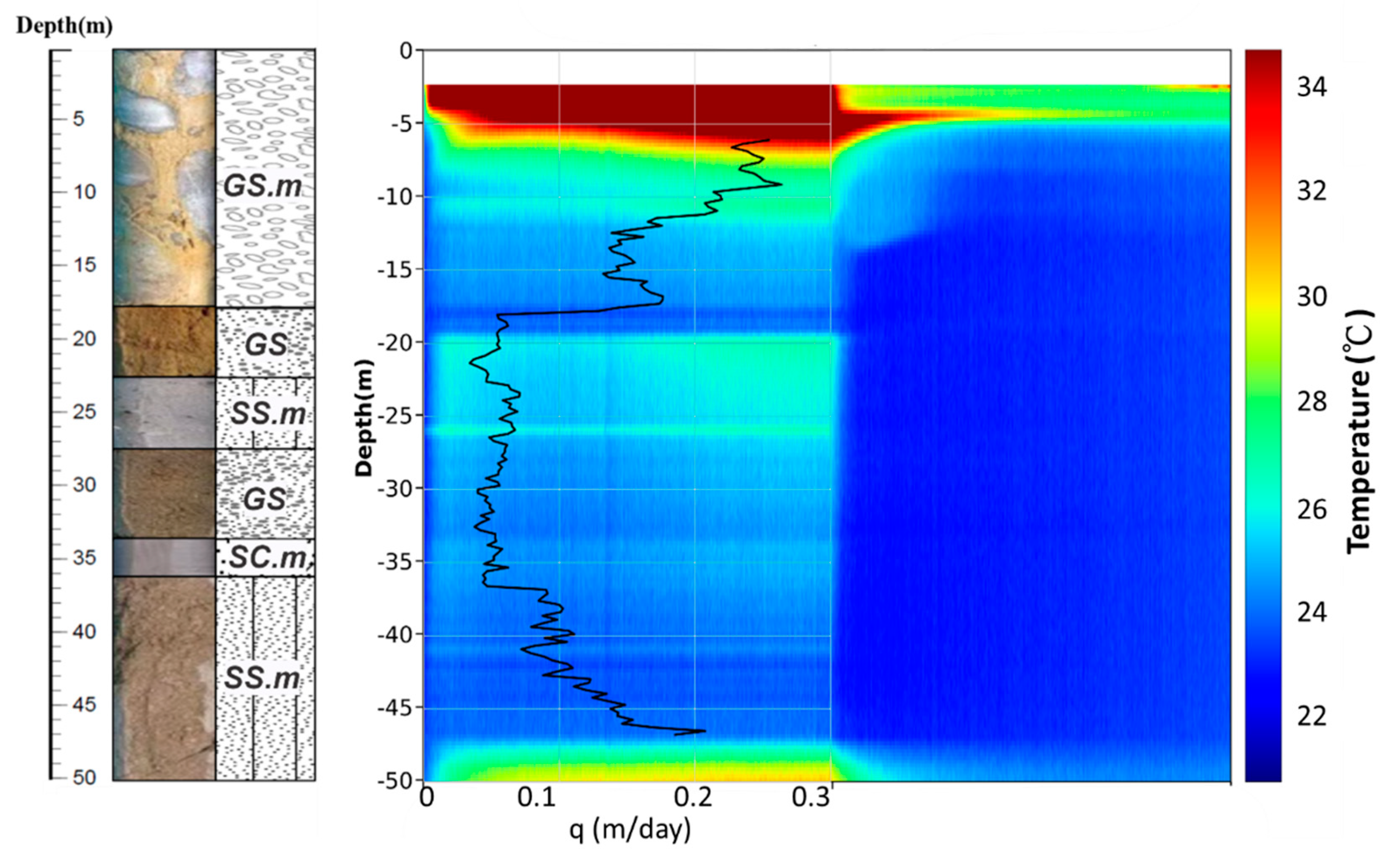

Table 1.
Specifications of the FODTS system for the study.
| Resolution | Range | Channels | Measurement Time | Fiber Type | Referencing | |
| Sampling | Temperature | |||||
| 20 cm | 0.01 ℃ | 0-5 km | 4 | sec | multimode | X2 PT-100 probes |
Table 2.
Scenarios of the active heating tests.
| Case |
Heating Power (kw) |
Duration (hr) | Tidal condition | ||
| Heating | Cooling | Heating | Cooling | ||
| Case 1 | 4.8、3.5、2.2 | 4 | 0 | High | - |
| Case 2 | 3.5 | 4 | 9 | High | Low |
| Case 3 | 3.5 | 4 | 9 | Low | High |
| Case 4 | 3.5 | 12.5 | 12 | Low to High | Low to High |
| Case 5 | 3.5 | 12.5 | 12 | High to Low | High to Low |
Table 3.
Specifications of the SH-3 sensor for measuring thermal properties of the soil samples in the laboratory.
Table 3.
Specifications of the SH-3 sensor for measuring thermal properties of the soil samples in the laboratory.
| Item | Range | Accuracy |
| Conductivity | 0.02 – 2.00 W/(mK) | from 0.02 – 2.00 W/(mK) |
| Diffusivity | at conductivity above 0.2 W/(mK) from 0.10 – 0.20 W/(mK) | |
| Volumetric Specific Heat Capacity | at conductivities above 0.1 W/(mK) |
Table 4.
Thermal properties estimated from the core samples in the laboaratory.
| Depth | 0-18.0m | 18.0-22.5m | 22.5-26.7m | 27.5-34.0m | 34.0-36.0m | 36.0-50.0m |
| Thermal diffusivity | 0.350 | 0.435 | 0.335 | 0.494 | 0.494 | 0.609 |
| Volumetric heat capacity | 2.645 | 1.282 | 2.200 | 2.907 | 1.909 | 2.913 |
| Thermal conductivityW/(mK) | 1.976 | 0.655 | 0.800 | 0.550 | 0.943 | 1.773 |
Disclaimer/Publisher’s Note: The statements, opinions and data contained in all publications are solely those of the individual author(s) and contributor(s) and not of MDPI and/or the editor(s). MDPI and/or the editor(s) disclaim responsibility for any injury to people or property resulting from any ideas, methods, instructions or products referred to in the content. |
© 2024 by the authors. Licensee MDPI, Basel, Switzerland. This article is an open access article distributed under the terms and conditions of the Creative Commons Attribution (CC BY) license (http://creativecommons.org/licenses/by/4.0/).
Copyright: This open access article is published under a Creative Commons CC BY 4.0 license, which permit the free download, distribution, and reuse, provided that the author and preprint are cited in any reuse.


