Submitted:
15 November 2024
Posted:
15 November 2024
You are already at the latest version
Abstract
We demonstrate high-resolution single-pixel imaging (SPI) in the visible and near-infrared wavelength ranges using an SPI framework that incorporates a novel, dedicated sampling scheme and a reconstruction algorithm optimized for rapid imaging of highly sparse scenes at the native digital micromirror device (DMD) resolution of 1024x768. The reconstruction algorithm consists of two stages. In the first stage, the vector of SPI measurements is multiplied by the generalized inverse of the measurement matrix. In the second stage, we compare two reconstruction approaches: one based on an iterative algorithm and the other on a trained neural network. The neural network outperforms the iterative method when the object resembles the training set, though it lacks the generalizability of the iterative approach. For images captured at a compression rate of 0.34 percent, corresponding to a measurement rate of 6.8 Hz with a DMD operating at 22 kHz, the typical reconstruction time on a desktop with a medium-performance GPU is comparable to the image acquisition rate. This allows the proposed SPI method to support high-resolution dynamic SPI in a variety of applications, using a standard SPI architecture with a DMD modulator operating at its native resolution and bandwidth, and enabling real-time processing of the measured data with no additional delay on a standard desktop PC.
Keywords:
single-pixel imaging
; infrared imaging
; compressive imaging
; computational imaging
; image reconstruction algorithms
; deep learning
; signal processing )
1. Introduction
Single-pixel imaging (SPI) [1,2] has led to a multiplicity of novel ideas about image measurement at various wavelength ranges, spectral imaging, imaging through scattering media, 3D imaging etc. [3,4,5]. SPI is designed to capture images using a single detector, instead of millions of detectors (pixels) included in traditional cameras. This enables imaging in wavelength ranges where conventional multi-pixel sensor arrays are expensive or even unavailable (e.g., infrared [6,7,8,9,10], ultraviolet [11], terahertz [12,13], or X-ray [14]). Besides, SPI makes it possible to capture images through scattering or opaque media including fog, or biological objects, where conventional imaging techniques often fail due to light scattering.
High resolution SPI (in the meaning of the number of pixels) puts immense demands on the image modulation bandwidth and the widely available DMD (Digital Micromirror Device) modulators operating at frequencies on the order of 20 kHz are often used at actual resolutions between 32x32 and 256x256, which is a fraction of their capability. In fact, with no compression and in a most straightforward differential imaging mode with a doubled number of expositions, SPI imaging at the resolution of 32x32 pixels is possible at only 10 Hz (since displaying patterns at 20 kHz takes s). This is not useful for practical applications. However, compressed SPI imaging has been shown many times at resolutions of 256x256 at frequencies between 5-15 Hz [10,15,16,17,18,19]. Unfortunately at high compression, the image reconstruction becomes computationally demanding. In this paper we push SPI imaging with DMD modulator to its limits, going for the native binary mode resolution, with efficiently implemented differential sampling and image reconstruction. The cost of this approach is to accept an extreme compression rate, and only sparse images can be reconstructed in an accurate way.
In recent years, there has been growing interest in applying deep learning methods to compressive SPI [20]. In [16], an end-to-end solution is proposed, where a convolutional autoencoder generates sensing patterns and reconstructs images from sparse SPI measurements in real time. Recent studies have explored the use of neural networks (NN) in SPI systems, either for end-to-end image reconstruction [21,22,23] or as denoising tools that complement other reconstruction methods [24,25]. The latter approach offers more flexibility, as the NN can be easily adjusted to work with various sampling schemes, compression levels, and changing measurement conditions. Additionally, there is growing interest in combining convolutional and recurrent NN to reconstruct temporal sequences of images from dynamic compressive measurements [26,27]. Although neural networks provide flexible, fast, and increasingly accurate solutions to inverse problems, they also have notable disadvantages. The training process is typically time-consuming and demands significant GPU power and memory. Moreover, to achieve high-quality reconstructions and sufficient generality, a neural network must be trained on large, diverse datasets, which can pose a challenge in some scenarios. To address these issues, there has been interest in exploring the possibility of applying untrained neural networks to SPI image reconstruction [28,29,30].
In this paper, we propose a framework for fast, high-resolution single-pixel imaging applicable to spatially sparse objects. This work extends our previous study [31,32], where we introduced a sampling scheme based on image maps and a two-stage image reconstruction approach. The sampling is now modified to distribute information about the mean value of the object across all sampling patterns. The iterative reconstruction algorithm is reformulated with minor adjustments in matrix form for more straightforward implementation on graphical processing units (GPUs). Additionally, we have developed Python code using the PyTorch module, enabling GPU execution. We also introduce an alternative second-stage reconstruction method based on a proposed neural network, implemented in PyTorch. This latter approach is significantly faster but lacks the generality of the iterative algorithm. Finally, the proposed algorithms are validated in an optical setup with two parallel channels, with detectors operating in the VIS and NIR wavelength ranges, respectively.
The paper is organized as follows. In the Materials and Methods section, we provide separate subsections to explain the consecutive elements of the SPI framework. In SubSection 2.1 and SubSection 2.2, we describe the development of sampling patterns and the motivation behind this approach. In SubSection 2.3 , we explain the initial stage of the reconstruction algorithm, which relies on the generalized inverse of the measurement matrix. SubSection 2.4 and SubSection 2.5 detail the two alternative approaches for the second reconstruction stage, and SubSection 2.6 describes the optical setup. In the Results section, we demonstrate cases where the proposed SPI framework produces high-resolution results, discuss various noise sources, and outline the computational and bandwidth requirements and limitations. Finally, we present our experimental results. The paper concludes with a summary in the Discussion section.
2. Materials and Methods
Sampling patterns and the image reconstruction algorithm are the two components that define any SPI framework. They are often independent, and various image reconstruction algorithms may be used in conjunction with different sampling patterns [4,12,33,34]. The block diagram of the proposed SPI imaging framework is shown in Figure 1, and the corresponding SPI optical setup is shown in Figure 2. The details of the SPI operation are presented in the following subsections.
2.1. Sampling Patterns
The type of image sampling is tied to the hardware used for spatial modulation. If DMD technology is used for this purpose, the sampling patterns should be binary, as the DMD mirrors inherently have only two states. Using grayscale modulation requires introducing spatial or temporal multiplexing, which occurs at the cost of the native DMD resolution or bandwidth [35]. The DMD bandwidth is also harnessed by utilizing differential projection [35], a commonly used technique that improves SNR, removes background light from the detector signal, and enables the display of both positive and negative patterns present in, e.g., Walsh-Hadamard matrices. However, these objectives can largely be achieved by adding a single pattern to those displayed, rather than doubling their number [36].
There are other important challenges introduced in a realistic optical setup that are not present in a purely digital experiment. These include the need for noise-mitigating techniques such as differential or complementary detection [37,38,39], as well as maintaining a consistent detection signal range throughout the measurement [10]. The latter suggests that it is inadvisable to combine, in a single measurement, sampling patterns where all pixels are in a single state with those where approximately half of the pixels share the same state. Otherwise, the experiment results in suboptimal usage of the detector’s dynamic range and A/D converter’s bit-depth for signal acquisition. Additionally, a signal obtained with a small number of pixels in the on-state tends to be weak in low-light environments and does not take advantage of Fellgett’s [40,41] multiplex advantage, which is particularly important in the infrared wavelength range.
To address these hardware-driven requirements, we propose a specific algorithmic procedure for constructing sampling patterns. The patterns are binary, each with approximately half of the pixels in the on-state. They are inherently differential, meaning that the measurement is based on the difference between the measurements of consecutive patterns. This eliminates any constant bias from the background or inactive areas of the DMD. Finally, the measurement provides data equivalent to a different measurement that would include patterns with a small number of pixels in one of the states. This is significant for identifying empty regions in the object area, which forms the basis for high compression utilization.
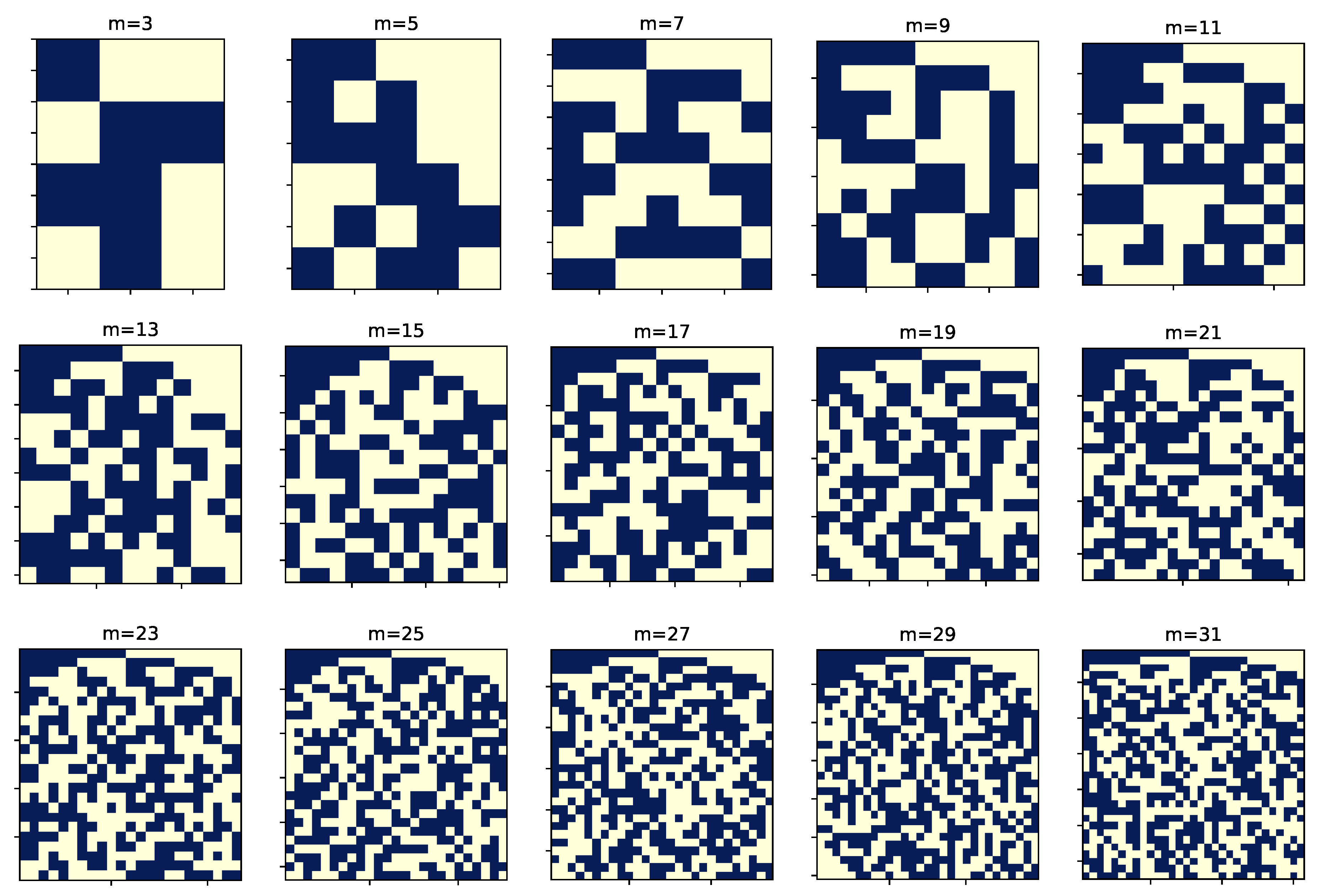
The process of preparing the sampling patterns and storing them in the measurement matrix is described in Algorithm 1. The entry point to the algorithm is a set of image plane partitions (divisions) into subareas or regions. These partitions are introduced in the form of image maps. The maps are somewhat arbitrary and may be object-specific. There is considerable flexibility in choosing the maps; for instance, by analogy to foveated SPI imaging [18,42,43], they can be adjusted to improve sampling quality in specific regions of interest at the expense of other areas [32]. The typical feature size of the regions can also be aligned with specific object feature sizes and shapes. Here, we use uniformly distributed maps with varying characteristic sizes. Sample maps are shown in Figure 3. We usually take maps, each with regions. Then, the algorithm encodes a sequence of binary full-resolution patterns. This corresponds to the sampling ratio (compression ratio) of %.
| Algorithm 1 Construction of a binary measurement matrix from image maps. |
|
Input: - matrix containing l maps with pixels
Input: - vector of length n with random integer values in the range
Input: - a look-up table; binary matrix , such that is full rank. Here is finite difference operator that subtracts matrix rows.
Output: - measurement matrix with rows containing binary patterns with n pixels each
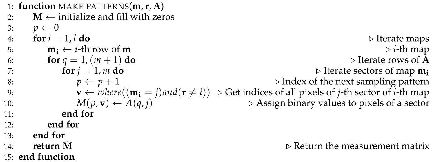
|
Samples of encoded patterns are shown in Figure 4. Encoding or translating image maps into patterns involves using a lookup table, which is described in the next subsection. The lookup table used throughout this paper is shown graphically in Figure 5.
Algorithm 1 is similar, but not identical, to the one we proposed previously [31,32]. There is a small change that affects the way the mean value of the object is encoded in the sampling patterns. Previously, we had been dropping some rows from the lookup table when translating the second and subsequent maps into patterns. This approach removed redundancy in the sampling. However, the disadvantage was that it allowed the recovery of the mean value of the object from the first sampling patterns. Since the mean value of the object influences all pixels in the reconstructed image, this type of sampling resulted in a very non-uniform distribution of values in the generalized inverse matrix.
Currently, Algorithm 1 processes all the maps in the same way, distributing the information about the mean value of the object across all sampling patterns. As a result, the inverse matrix has improved uniformity.
2.2. Differential Multiplexing
The mechanism of differential multiplexing is governed by the multiplexed pattern encoding algorithm, with a crucial role played by the dedicated binary lookup table. The translation of image maps into sampling patterns is described by Algorithm 1. Pattern encoding is performed using a lookup table, which is a binary matrix . The table is scanned row by row, with its columns indicating which map regions should be included in the encoded sampling pattern. The encoding mechanism should ensure that the differences between consecutively created binary patterns convey the same information about the sampled objects as would be obtained through sampling using individual map regions. Therefore, the lookup table must satisfy certain mathematical properties. Specifically, its rows should contain approximately equal numbers of zeros and ones, and a matrix formed by subtracting its rows should be a full-rank square matrix. These conditions cannot be achieved for even m, so the matrix has an odd number of columns. A gallery of lookup tables of different sizes is shown in Figure A1. Despite these conditions, there is still room for further optimization, and we search for matrices with the smallest possible determinant . As a result, the lookup tables we use are derived from brute-force numerical optimization. It is worth noting that the columns of the lookup tables can be freely reordered, but not the rows. In fact, the regions of each map can be reordered as desired.
Finally, we note that in a non-differential measurement, we could use a square Hadamard matrix instead of our lookup tables, as Hadamard matrices are inherently full-rank and have an equal number of the two binary values (with the first row different). In fact, Hadamard matrices have a well established position in multiplexed measurements. However, Hadamard matrices include both positive and negative values (e.g., ), which introduces additional challenges when displaying them on a DMD. To address this, one would need to double the number of exposures, thus reducing the effective DMD bandwidth. Therefore, the proposed matrices are useful in designing an inherently differential multiplex measurement that is equivalent to binary sampling with patterns occupying small parts of the image (See Figure 6) and together forming l independent partitions of the image surface. In many cases, they may be better suited for conducting a multiplexed measurement than Hadamard matrices.
2.3. Initial Image Reconstruction
The measurement of an object in SPI imaging is usually expressed mathematically using a concise measurement equation, which in a noise-free situation may be written as
Here, denotes the object, such as a 2D image, with pixels gathered into a single vector. is the measurement matrix, whose rows contain the sampling patterns. Finally, is the measurement vector. A refined version of this equation would also include signal-dependent and signal-independent noise. There are various ways to conduct a differential measurement. In the present work, we calculate the difference of subsequent elements in the measurement vector, i.e., , and use only for image reconstruction. Here, denotes a finite difference operator that subtracts subsequent rows of a matrix or subsequent elements of a vector. Any constant DC component, such as one originating from background light, is eliminated from . The SPI reconstruction algorithm should then be able to recover from . In a compressive measurement, where is a rectangular matrix with more columns than rows, this recovery is usually ambiguous and approximate.
Most SPI image reconstruction algorithms are either iterative or based on applying the pseudoinverse of the measurement matrix to the measured signal, i.e., . This is particularly straightforward when the measurement matrix is semi-orthogonal. An even simpler situation arises when it corresponds to a fast linear transform such as DCT, Fourier, or Walsh-Hadamard transforms. Our approach is slightly different. We work with the full form of the measurement matrix and find its generalized inverse . The Moore-Penrose pseudoinverse is an example of a matrix’s generalized inverse, but it is not the only one. Inverting (with generalized inverse) is only possible at very high compression rates, i.e., when the number of rows of the matrix is small.
is calculated before SPI imaging, and it may require a significant amount of memory (we typically work with 10 GB inverse matrices). However, the image reconstruction is fast because it is based on a simple matrix-vector multiplication. Since we assume a differential measurement, we need an inverse matrix of the form .
For the generalized inversion (g), one could use the pseudoinverse, but it is preferable to use a regularized pseudoinverse. In our case, this is:
where is the measurement matrix, is the 2D Fourier Transform, is the finite difference operator, and is a diagonal nonnegative regularizing term [31]. Matrix is defined as in Ref. [15],
where and are used to tune the properties of the regularization and are the spatial frequencies. As a rule of thumb, we assume that and .
The reconstructed image is then calculated as
where
The function removes the negative part form the reconstructed image which we consider to be a reconstruction artifact. At lower resolutions, could be the final result of SPI imaging. Since we are interested in high-resolution SPI, this first-stage reconstruction serves as the starting point for further enhancement with Algorithm 2 or a neural network.
2.4. Reconstruction Enhancement with an Iterative Algoritm
The proposed Algorithm 2 enhances the initially reconstructed image by leveraging two key elements. First, since the initial reconstruction is based on the generalized inverse of the measurement matrix, exactly fulfills the measurement equation (1). Second, the construction of the binary measurement matrix ensures that sampling with this matrix is mathematically equivalent to using patterns that correspond to all individual regions of all image maps.
| Algorithm 2 Image reconstruction from a compressive measurement. |
|
Input: - measurement vector of length k (it i assumed that , where is the image size in pixels, and that the measurement equation is , where is the measured image, and is the binary measurement matrix)
Input: - binary array. at pixels p belonging to region j of map i unless .
Input: - array of l matrices with dimensions . Here is the generalized matrix inverse g applied to the measurement matrix after taking the differences of its rows with operator
Input: - the initial image reconstruction vector of size (set by us to the initial reconstruction result but may also be filled with constant positive values)
Input: - learning rate (we took )
Output: - vector of size n with the reconstructed image
|
Algorithm 2 iteratively processes all image maps, applying corrections to the mean values of pixels within the regions of each map. Because these regions are non-overlapping, they can be processed in parallel. A similar reconstruction method was used in Ref. [31]; however, here we introduce a parameter, the learning rate , which typically improves convergence in the presence of noise. In this paper, we assume .
An important property of this algorithm is its efficient elimination of empty (zero-valued) regions from the reconstructed image. As a result, for spatially sparse images, it improves image quality in regions containing objects. This improvement is achieved because the limited information in the compressed measurement is directed toward reconstructing only the non-empty regions of the image. This approach can be viewed as complementary to adaptive sampling; however, adaptive sampling is technically more complex, requiring additional logic in the measurement stage and posing challenges in generating adaptively high-resolution patterns at the DMD frame rate. In contrast, our approach relies on predefined patterns for measurement and separates the measurement process from the reconstruction phase.
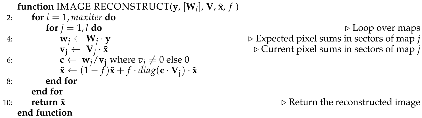
2.5. Reconstruction Enhancement with a Neural Network
In an alternative approach to Algorithm 2, we explore the application of a neural network to enhance the reconstruction quality. The proposed network bears some resemblance to the U-Net architecture; however, instead of concatenation in the skip connections, we employ weighted data summation, where the weights are learned parameters of the network. This modification enables the network to balance the influence of input data and extracted features on the final output, placing it in a functional space between a U-Net and an autoencoder.
Figure 7.
Block diagram of the neural network architecture. The network consists of 8 convolutional blocks arranged in a U-Net architecture, with the first 4 blocks forming the contracting path and the remaining 4 blocks forming the expanding path. Each convolutional block comprises a convolutional layer, a rectified linear unit (ReLU) nonlinear activation, and a batch normalization (BN) layer. Two-dimensional max pooling is applied in the contracting path to reduce the spatial size of the data, while nearest-neighbor interpolation is used in the expanding path to upsample the data. Additionally, weighted skip connections, with learned weights , combine features from matching blocks in both paths to improve data fidelity. The skip connections are applied directly after the convolutional layers and before the ReLU activations.
The neural network is trained simultaneously on two handcrafted image datasets. The first dataset comprises binary, high-resolution images of line art, while the second dataset contains images of randomly placed and scaled handwritten digits drawn from the MNIST dataset. The training dataset consists of 30,000 images, drawn equally from both datasets, and is randomly regenerated in each training epoch to enhance the variety of the training data. The evaluation dataset, which is precalculated, contains 6,000 images, also drawn equally from both datasets. Notably, the handwritten digits included in the evaluation dataset are not used for generating the training images. All images in both datasets have a resolution of pixels and are normalized to pixel values in the range .
The neural network is designed to perform the second stage reconstruction as an alternative to using Algorithm 2. The input data consists of initially reconstructed images obtained by applying Eq. (5) to simulated SPI measurements. To model realistic experimental conditions, we introduce additive Gaussian noise to the measurement. The network is trained to optimize a joint loss function:
where denotes the mean squared error, x represents the pixel values of the ground truth image, is the output of the neural network, v and are the sums of pixel values within all sectors of the maps calculated for images x and , respectively, and is a weight parameter empirically adjusted during training.
2.6. Optical Set-Up
We validated the performance of the proposed algorithm by implementing the SPI optical setup using a pixel DMD (Vialux V-7001 XGA with DLP7000), which splits the light beam into two separate detectors: an uncooled Thorlabs PDA100A2 silicon photodiode for the 300-1100 nm range, and a thermoelectrically cooled VIGO Photonics PVI-4TE-5 detector for the 1100-3000 nm range. The schematic is shown in Figure 2. Light from a thermal source passes through a test pattern composed of a series of holes in a nontransparent metal foil, with the object observed in transmission mode.
To minimize chromatic aberration, we first used a set of gold-coated parabolic mirrors as the imaging system. We also tested an alternative setup using fused silica lenses. The parabolic mirrors provide better signal-to-noise ratio (SNR) for the infrared (IR) optical channel, while the glass lenses offer higher image resolution in the visible light range. The signal is digitized using a 14-bit digital oscilloscope (Picoscope 5000) with a sampling rate of 128 ns. Since the DMD frequency is lower, the measurement vector is obtained from these samples by averaging.
3. Results
3.1. Image Acquisition and Reconstruction Times and Computational Requirements
Throughout this paper, we assume an image resolution of , with the object being sampled at a high compression rate of %, requiring 3200 binary patterns for sampling. The DMD operates at 22 kHz, resulting in an image acquisition frequency of Hz. Our image reconstruction algorithm is implemented in Python, utilizing the NumPy and PyTorch libraries, and is capable of running on both CPU and GPU processors. Due to the high memory demands, we used a GPU with 24 GB of memory (NVIDIA GeForce RTX 3090). Specifically, the measurement matrix and the inverse matrix each occupy 10 GB in 32-bit floating-point format. This suggests that further increasing the number of sampling patterns at the same resolution may present challenges for this framework and could require either a scanning strategy or parallel SPI measurements in lower-resolution blocks.
The initial reconstruction takes 16 ms and can be performed on the fly without noticeable impact on the DMD acquisition rate, reducing the rate from Hz to Hz. The second-stage reconstruction using the neural network takes 26 ms (including the initial reconstruction stage), resulting in an SPI rate of Hz. The iterative algorithm is slower, requiring approximately 50 ms per iteration, which limits real-time applications to one or two iterations; performing 50 iterations would take s. Additionally, due to the GPU architecture, images from two or more channels can be reconstructed in parallel without additional time penalty, leveraging batch processing implemented in PyTorch. Without a GPU, processing times are significantly longer. On an Intel i7-11700K CPU, the initial reconstruction takes 350 ms, and the iterative algorithm is much slower, taking s per iteration (although computation speed could improve by up to tenfold with a Numba-based implementation, [31]). In summary, for applications that are not time-critical, Algorithm 2 may be applied with multiple iterations. At the same time, only a GPU-based approach—either using the second-stage reconstruction with the NN or a single iteration of Algorithm 2 enables image acquisition and reconstruction at over 6 Hz at a resolution of without hindering the DMD acquisition rate.
3.2. Effect of Compression Noise, Background Noise, and Detector Noises on Imaging
Eliminating additive background noise is critical in optical SPI. This noise may include a constant or slowly varying bias in the detector signal due to the dark current, background illumination, or reflections from inactive parts of the DMD, as well as variations in the light source intensity. In infrared imaging, the changing temperature of the setup, and particularly of the DMD, also contributes to a slowly varying additive background signal. Background noise is usually reduced through differential or interferometric techniques, such as projecting negated DMD patterns or using complementary detection of the two beams reflected by the DMD in the directions corresponding to the on and off states of the mirrors. In our case, we incorporate the differential mechanism in the way we construct sampling patterns and measurements. Thus, the reconstructed image is invariant with respect to adding any constant value to the detection signal. This approach also allows us to use the AC coupling of the DAQ, although this type of high-pass filtering is not entirely transparent to the image reconstruction outcome.
A variety of other noise sources also affect SPI imaging, and the impact of one source may often become dominant. We now discuss the effect of compression noise and detector additive noise. SPI imaging at extremely high compression rates is naturally strongly influenced by compression noise. The impact of this noise depends significantly on the structure of the object, particularly on the presence of empty (zero-valued) areas within the object image. To our knowledge, there are no existing test image datasets categorized by spatial sparsity, making it difficult or impossible to use standard image archives for the analysis in this paper. Consequently, we first selected three images with different properties to illustrate the typical behavior of the presented SPI method in the presence of different sparsity levels. We then created synthetic images based on the MNIST database with added Gaussian noise for further comparisons.
In Figure 8 and Figure 9, we demonstrate the role of compression noise in SPI imaging with three example images: the Siemens star, which is a dense grayscale test object with no empty regions; a limited-field-of-view Siemens star; and a sparse line-art image. Compression noise is the only type of noise present in this analysis. An approximate reconstruction result is obtained with the initial reconstruction method, similar to what could be achieved with low-resolution SPI imaging (e.g., 128×128 or 256×256 at most). For the grayscale image, no significant improvement is achieved with the iterative algorithm. However, Algorithm 2 significantly improves the quality of the other two images, achieving up to the DMD resolution (1024×768). In Figure 8, we also measure the reconstruction quality using two standard criteria: peak signal-to-noise ratio (PSNR) and structural similarity (SSIM). The notable differences in these criteria reveal that averaging these measures across a range of standard database images would obscure information about the properties of imaging sparse objects.
In Figure 9, we show the convergence of PSNR and SSIM for the same three objects as a function of the number of iterations in Algorithm 2. In addition to the data presented with solid lines, we show the same convergence when the initial reconstruction stage is omitted, which slightly improves computation time and significantly reduces memory requirements due to the large size of the inverse matrix . Results from this plot indicate that typically the first 1–5 iterations are sufficient to nearly reach the final image quality. The importance of the first stage reconstruction largely depends on the type of image; it is especially crucial for the grayscale Siemens star, although it also plays a role in achieving convergence of PSNR and SSIM for the other two objects.
The role of additive detector noise is depicted in Figure 10, Figure 11 and Figure 12. An often overlooked source of additive noise is the limited bit resolution of the detection system introduced by the DAQ. Depending on the sampling patterns, the required dynamic range of the detector may be utilized more or less efficiently. A common issue in SPI is that, aside from patterns containing approximately half of the pixels in either on or off states, there also appear frames with all pixels switched on or off. As a result, the quality of the measurement depends on fine signal changes between consecutive projected patterns, yet some signal points deviate significantly from typical values, which imposes unnecessary constraints on the DAQ bit resolution. We avoid this issue by properly constructing the measurement matrix. Nevertheless, the DAQ bit resolution does influence the final SPI quality, as shown in Figure 10, which illustrates the relationship between PSNR and SSIM versus the DAQ bit resolution.
We note that due to its randomness, DAQ discretization noise exhibits properties similar to additive Gaussian noise, unless very few bits are effectively used in the signal’s discretization. According to the results in Figure 10, at resolutions below 12 bits, limited bit resolution begins to impact image quality more than compression. For this reason, in the optical experiments, we use at least 14-bit discretization in the measurement.
A comparison of the performance of the two second-stage reconstruction methods (Algorithm 2 and NN) in the presence of additive Gaussian detector noise is shown in Figure 11. This comparison is performed on a set of images similar (but not identical) to those included in the NN training set. At an SNR of 45 dB, both methods perform well and achieve high-resolution SPI imaging, with the NN method being significantly faster and yielding better quantitative results in terms of SSIM and PSNR. However, for images that differ from the training data, the NN often introduces significant artifacts, while Algorithm 2 maintains good performance even for arbitrarily designed images. In Figure 12, we compare these two methods more systematically, using PSNR, SSIM, and the and loss function components, averaged over a set of 1000 images and plotted against the measurement SNR.
3.3. Experimental Results
Real-world visible and infrared scenes often include dense grayscale objects. While the SPI method proposed in this paper can be applied to dense images, high-resolution imaging is only achievable for sparse objects. For dense objects, an alternative measurement matrix—such as one based on binarized DCT patterns—may be more suitable and could improve the overall quality of reconstruction. Sparse objects, in this context, include those obtained through phase contrast or polarization contrast, as well as objects observed over a known background that can be subtracted from the measurement, or scenes with the field of view reduced by vignetting to a selected region of interest.
In our example, a sparse object is represented by a metal foil with small holes arranged in the shape of the Faculty logo. In our experimental setup, two measurement vectors are captured simultaneously by two detectors operating in different wavelength ranges. These detectors measure light intensities reflected from the DMD in two directions corresponding to the on and off states of the micromirrors. Such an arrangement could support complementary detection—a technique for enhancing signal-to-noise ratio (SNR) and removing the DC component from the signal. Since our measurement is inherently differential, we can utilize the two channels independently. Given that the image reconstruction method is invariant to adding a constant to the signal, data from both channels are processed identically, with the only difference being that signals obtained with mirrors in the negated state (in relation to the measurement matrix, in a boolean sense) also need to be negated (in the sense of multiplication by -1). Grayscale images from the two channels are then used to construct a false-color image.
4. Discussion
We propose and compare two methods for SPI imaging at the native DMD resolution. Both methods use the same differential multiplexing sampling scheme and an initial reconstruction stage based on the dot product with the regularized generalized inverse of the measurement matrix (according to Eq. (4)). The second reconstruction stage is either based on an iterative Algorithm 2 or a neural network, inspired by the convolutional U-Net architecture, as shown in Figure 7. The proposed SPI approaches rely on extremely high compression, which is dictated by the limited bandwidth of DMD modulators. This restricts the possibility of high-resolution reconstruction to spatially sparse images with limited information content. Dense grayscale images, on the other hand, can only be reconstructed with lower accuracy.
For NN-based reconstruction, high-quality results are achieved only for images similar to those in the training set. The NN is trained on line-art images and transformed alphanumeric objects from the MNIST dataset, and may not perform well on other types of objects or images at different resolutions without further training or modifications. In contrast, Algorithm 2 can be directly applied to different resolutions and more general sparse image types.
The proposed method is validated in an optical setup with two detectors operating in the VIS and NIR wavelength ranges. Object sampling at a compression rate of 0.34% reconstructions, which are outside the scope of this paper. Both the NN and Algorithm 2, when used with a single iteration, can reconstruct images at a rate that does not hinder the acquisition frame rate. However, Algorithm 2 with multiple iterations can still be applied in practical applications, with a time penalty of 50 ms per iteration on a GPU.
One advantage of Algorithm 2 is its ability to identify empty regions of the object, which helps improve reconstruction accuracy in areas containing actual content. In this way, the proposed high-resolution SPI framework offers an alternative to adaptive sampling methods, which are challenging to implement. Given the low resolution of most current SPI systems (typically between 32×32 and 256×256), which limits their potential to replace traditional high-resolution cameras, we consider this work an important step toward enabling practical SPI applications in a variety of fields.
Author Contributions
Methodology, R.K., A.P. ; experimental set-up, R.S., P.W. ; neural network A.P.; other software, R.K, A.P.,R.S.; validation, M.C., K.S., A.P.; dataset resources, K.S.; writing, review and editing, R.K, A.P, R.S., P.W. et al. visualization, M.C., A.P., K.S., R.S.; supervision, R.K.; project administration, A.P.; funding acquisition, A.P. All authors have read and agreed to the published version of the manuscript.
Funding
This research was partly funded by National Science Center, Poland UMO-2019/35 /D/ST7/03781 (AP).
Data Availability Statement
Datasets with image maps, sampling patterns, inverse matrix etc may be downloaded from the repository of the University of Warsaw [44]. More information and parts of the source code may be provided at a reasonable request.
Conflicts of Interest
The authors declare no conflicts of interest.
Abbreviations
The following abbreviations are used in this manuscript:
| SPI | Single-pixel imaging |
| DMD | Digital micromirror device |
| NN | Neural network |
| PSNR | Peak signal to noise ratio |
| SSIM | Structural similarity index |
| MSE | Mean square error |
| SNR | Signal-to-noise-ratio |
Appendix A
In this Appendix, we present a gallery of the optimized lookup matrices for binary differential multiplexed measurements. These matrices were originally introduced in [31]. In this presentation, in addition to displaying them graphically, we have applied a systematic column ordering to the matrices to facilitate better comparison among them and with Hadamard matrices. The role of the lookup tables in designing differential multiplexed measurements is discussed in Section 2.2.
Figure A1.
A gallery of lookup-tables of different sizes for differential multiplexed measurements. Note that the last matrix i.e. for is equivalent to the one in Figure 5 but with a different column ordering. In this figure, the columns are ordered by sorting the values in rows starting from the top row (but preserving the rows sorted earlier.)
References
- Duarte, M.F.; Davenport, M.A.; Takhar, D.; Laska, J.N.; Sun, T.; Kelly, K.F.; Baraniuk, R.G. Single-pixel imaging via compressive sampling. IEEE Sig. Proc. Mag. 2008, 25, 83–91. [Google Scholar] [CrossRef]
- Candes, E.J.; Romberg, J.K.; Tao, T. Stable signal recovery from incomplete and inaccurate measurements. Commun. Pure Appl. Math. 2006, 59, 1207–1223. [Google Scholar] [CrossRef]
- Osorio Quero, C.A.; Durini, D.; Rangel-Magdaleno, J.; Martinez-Carranza, J. Single-pixel imaging: An overview of different methods to be used for 3D space reconstruction in harsh environments. Rev. Sci. Instrum. 2021, 92, 111501. [Google Scholar] [CrossRef] [PubMed]
- Gibson, G.M.; Johnson, S.D.; Padgett, M.J. Single-pixel imaging 12 years on: a review. Opt. Express 2020, 28, 28190–28208. [Google Scholar] [CrossRef]
- Edgar, M.P.; Gibson, G.M.; Padgett, M.J. Principles and prospects for single-pixel imaging. Nat. Photonics 2018, 13, 13–20. [Google Scholar] [CrossRef]
- Mahalanobis, A.; Shilling, R.; Murphy, R.; Muise, R. Recent results of medium wave infrared compressive sensing. Appl. Opt. 2014, 53, 8060–8070. [Google Scholar] [CrossRef]
- Radwell, N.; Mitchell, K.J.; Gibson, G.M.; Edgar, M.P.; Bowman, R.; Padgett, M.J. Single-pixel infrared and visible microscope. Optica 2014, 1, 285–289. [Google Scholar] [CrossRef]
- Denk, O.; Musiienko, A.; Žídek, K. Differential single-pixel camera enabling low-cost microscopy in near-infrared spectral region. Opt. Express 2019, 27, 4562. [Google Scholar] [CrossRef]
- Zhou, Q.; Ke, J.; Lam, E.Y. Near-infrared temporal compressive imaging for video. Opt. Lett. 2019, 44, 1702. [Google Scholar] [CrossRef]
- Pastuszczak, A.; Stojek, R.; Wróbel, P.; Kotyński, R. Differential real-time single-pixel imaging with Fourier domain regularization - applications to VIS-IR imaging and polarization imaging. Opt. Express 2021, 29, 2685–26700. [Google Scholar] [CrossRef]
- Ye, J.T.; Yu, C.; Li, W.; Li, Z.P.; Lu, H.; Zhang, R.; Zhang, J.; Xu, F.; Pan, J.W. Ultraviolet photon-counting single-pixel imaging. Applied Physics Letters 2023, 123, 024005. [Google Scholar] [CrossRef]
- Stantchev, R.; Yu, X.; Blu, T.; Pickwell-MacPherson, E. Real-time terahertz imaging with a single-pixel detector. Nat. Commun. 2020, 11, 2535. [Google Scholar] [CrossRef] [PubMed]
- Zanotto, L.; Piccoli, R.; Dong, J.; Morandotti, R.; Razzari, L. Single-pixel terahertz imaging: a review. Opto-Electron Adv. 2020, 3, 200012. [Google Scholar] [CrossRef]
- Olbinado, M.P.; Paganin, D.M.; Cheng, Y.; Rack, A. X-ray phase-contrast ghost imaging using a single-pixel camera. Optica 2021, 8, 1538–1544. [Google Scholar] [CrossRef]
- Czajkowski, K.; Pastuszczak, A.; Kotynski, R. Real-time single-pixel video imaging with Fourier domain regularization. Opt. Express 2018, 26, 20009–20022. [Google Scholar] [CrossRef]
- Higham, C.; Murray-Smith, R.; Padgett, M.; Edgar, M. Deep learning for real-time single-pixel video. Sci. Rep. 2018, 8, 2369. [Google Scholar] [CrossRef]
- Rizvi, S.; Cao, J.; Zhang, K.; Hao, Q. DeepGhost: real-time computational ghost imaging via deep learning. Sci. Rep. 2020, 10, 11400. [Google Scholar] [CrossRef] [PubMed]
- Wang, G.; Deng, H.; Ma, M.; Zhong, X.; Gong, X. A non-iterative foveated single-pixel imaging using fast transformation algorithm. Appl. Phys. Lett. 2023, 123, 081101. [Google Scholar] [CrossRef]
- Zhu, X.; Li, Y.; Zhang, Z.; Zhong, J. Adaptive real-time single-pixel imaging. Opt. Lett. 2024, 49, 1065–1068. [Google Scholar] [CrossRef]
- Zhang, Z.; Zheng, S.; Qiu, M.; Situ, G.; Brady, D.J.; Dai, Q.; Suo, J.; Yuan, X. A Decade Review of Video Compressive Sensing: A Roadmap to Practical Applications. Engineering 2024. [Google Scholar] [CrossRef]
- Ni, Y.; Zhou, D.; Yuan, S.; Bai, X.; Xu, Z.; Chen, J.; Li, C.; Zhou, X. Color computational ghost imaging based on a generative adversarial network. Opt. Lett. 2021. [Google Scholar] [CrossRef] [PubMed]
- Wu, H.; Wang, R.; Zhao, G.; Xiao, H.; Wang, D.; Liang, J.; Tian, X.; Cheng, L.; Zhang, X. Sub-Nyquist computational ghost imaging with deep learning. Opt. Express 2020, 28, 3846–3853. [Google Scholar] [CrossRef] [PubMed]
- Wang, F.; Wang, H.; Wang, H.; Li, G.; Situ, G. Learning from simulation: An end-to-end deep-learning approach for computational ghost imaging. Opt. Express 2019, 27, 25560–25572. [Google Scholar] [CrossRef]
- Wang, F.; Wang, C.; Deng, C.; Han, S.; Situ, G. Single-pixel imaging using physics enhanced deep learning. Photon. Res. 2022, 10, 104–110. [Google Scholar] [CrossRef]
- Tian, Y.; Fu, Y.; Zhang, J. Plug-and-play algorithms for single-pixel imaging. Optics and Lasers in Engineering 2022, 154, 106970. [Google Scholar] [CrossRef]
- Cheng, Z.; Lu, R.; Wang, Z.; Zhang, H.; Chen, B.; Meng, Z.; Yuan, X. BIRNAT: Bidirectional Recurrent Neural Networks with Adversarial Training for Video Snapshot Compressive Imaging. In Proceedings of the Computer Vision – ECCV 2020; Vedaldi, A.; Bischof, H.; Brox, T.; Frahm, J.M., Eds., Cham; 2020; pp. 258–275. [Google Scholar] [CrossRef]
- Qin, C.; Schlemper, J.; Caballero, J.; Price, A.N.; Hajnal, J.V.; Rueckert, D. Convolutional Recurrent Neural Networks for Dynamic MR Image Reconstruction. IEEE Trans. Med. Imaging 2019, 38, 280–290. [Google Scholar] [CrossRef]
- Li, Z.; Huang, J.; Shi, D.; Chen, Y.; Yuan, K.; Hu, S.; Wang, Y. Single-pixel imaging with untrained convolutional autoencoder network. Opt. Laser Technol. 2023, 167, 109710. [Google Scholar] [CrossRef]
- Liu, S.; Meng, X.; Yin, Y.; Wu, H.; Jiang, W. Computational ghost imaging based on an untrained neural network. Optics and Lasers in Engineering 2021, 147, 106744. [Google Scholar] [CrossRef]
- Wang, C.H.; Li, H.Z.; Bie, S.H.; Lv, R.B.; Chen, X.H. Single-Pixel Hyperspectral Imaging via an Untrained Convolutional Neural Network. Photonics 2023, 10. [Google Scholar] [CrossRef]
- Stojek, R.; Pastuszczak, A.; Wrobel, P.; Kotynski, R. Single pixel imaging at high pixel resolutions. Opt. Express 2022, 30, 22730–22745, (Codeavailableathttp://github.com/rkotynski/MD-FDRI). [Google Scholar] [CrossRef]
- Pastuszczak, A.; Stojek, R.; Wróbel, P.; Kotyński, R. Single pixel imaging at high resolution with sampling based on image maps. In Proceedings of the 2024 International Workshop on the Theory of Computational Sensing and its Applications to Radar, Multimodal Sensing and Imaging (CoSeRa); 2024; p. 86. [Google Scholar] [CrossRef]
- Zhao, W.; Gao, L.; Zhai, A.; Wang, D. Comparison of Common Algorithms for Single-Pixel Imaging via Compressed Sensing. Sensors 2023, 23. [Google Scholar] [CrossRef] [PubMed]
- Bian, L.; Suo, J.; Dai, Q.; Chen, F. Experimental comparison of single-pixel imaging algorithms. J. Opt. Soc. Am. A 2018, 35, 78–87. [Google Scholar] [CrossRef]
- Zhang, Z.; Ma, X.; Zhong, J. Single-pixel imaging by means of Fourier spectrum acquisition. Nat. Commun. 2015, 6, 6225. [Google Scholar] [CrossRef] [PubMed]
- Czajkowski, K.M.; Pastuszczak, A.; Kotynski, R. Single-pixel imaging with sampling distributed over simplex vertices. Opt. Lett. 2019, 44, 1241–1244. [Google Scholar] [CrossRef]
- Yu, W.K.; Liu, X.F.; Yao, X.R.; Wang, C.; Zhai, Y.; Zhai, G.J. Complementary compressive imaging for the telescopic system. Sci. Rep. 2014, 4, 5834. [Google Scholar] [CrossRef]
- Gong, W. Disturbance-free single-pixel imaging camera via complementary detection. Opt. Express 2023, 31, 30505–30513. [Google Scholar] [CrossRef]
- Yu, W.K.; Yao, X.R.; Liu, X.F.; Li, L.Z.; Zhai, G.J. Compressive moving target tracking with thermal light based on complementary sampling. Appl. Opt. 2015, 54, 4249–4254. [Google Scholar] [CrossRef]
- Fellgett, P. Conclusions on multiplex methods. J. Phys. Colloq. 1967, 28, C2–165. [Google Scholar] [CrossRef]
- Scotté, C.; Galland, F.; Rigneault, H. Photon-noise: is a single-pixel camera better than point scanning? A signal-to-noise ratio analysis for Hadamard and Cosine positive modulation. J. Phys. Photonics 2023, 5, 035003. [Google Scholar] [CrossRef]
- Phillips, D.B.; Sun, M.J.; Taylor, J.M.; Edgar, M.P.; Barnett, S.M.; Gibson, G.M.; Padgett, M.J. Adaptive foveated single-pixel imaging with dynamic supersampling. Sci. Adv. 2017, 3, e1601782. [Google Scholar] [CrossRef]
- Cui, H.; Cao, J.; Zhang, H.; Zhou, C.; Yao, H.; Hao, Q. Uniform-sampling foveated Fourier single-pixel imaging. Opt. Laser Technol. 2024, 179, 111249. [Google Scholar] [CrossRef]
- Sobczak, K.; Kotynski, R.; Stojek, R.; Pastuszczak, A.; Cwojdzinska, M.; Wróbel, P. Large datasets for high resolution single pixel imaging, 2024. Data repository of the Univ. of Warsaw. [CrossRef]
Figure 1.
Block diagram of the proposed high-resolution SPI framework. The blocks in the upper row show the preparation stage, involving the calculation of large matrices needed for object sampling and for the reconstruction of the SPI measurement afterward. The blocks in the bottom row describe the actual SPI measurement and reconstruction. In continuous SPI imaging, the bottom blocks are executed cyclically.
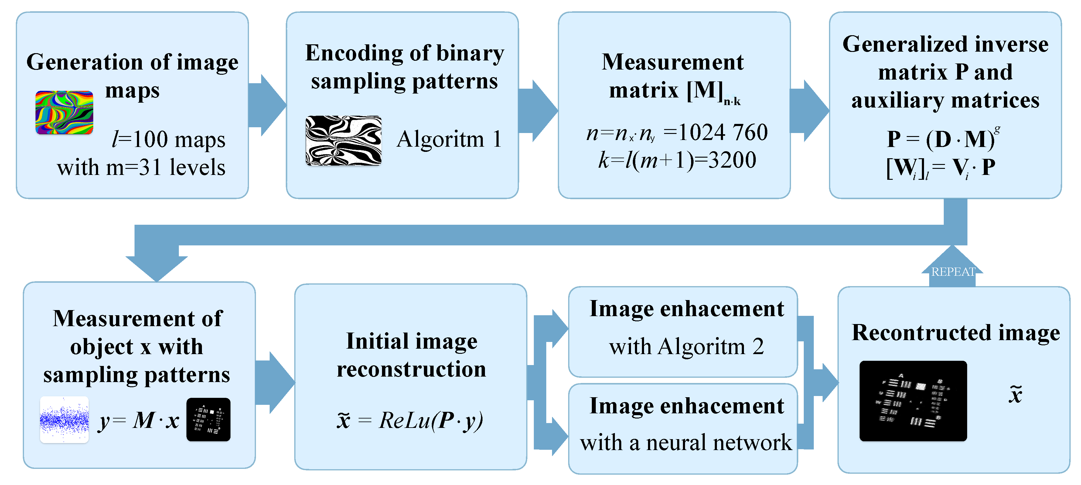
Figure 2.
SPI optical setup with a broadband light source, a DMD modulator operating in the native binary mode at up to 22 kHz, and two detectors—a VIS/NIR range Si amplified detector and a thermoelectrically cooled MCT detector for the NIR/MIR range. The detectors are placed in a complementary architecture, measuring the signal reflected by the DMD mirrors in either the "zero" or "one" positions.
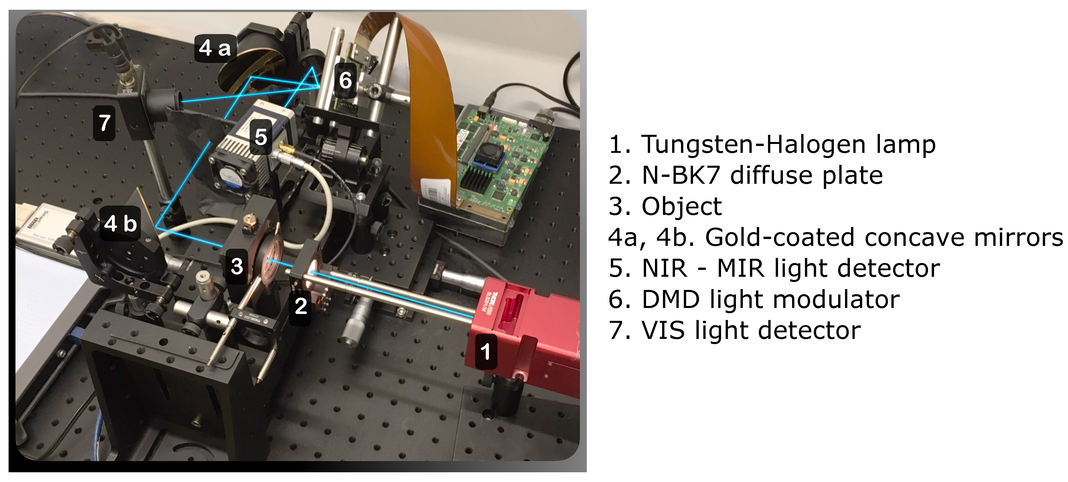
Figure 3.
Examples of high-resolution () image maps. The above 9-element sample is a subset taken from the -element set of maps. Every map includes different regions shown in different (false) colors. The characteristic feature size is different in each map. Each of the maps is used to create sampling patterns (see Algorithm 1).
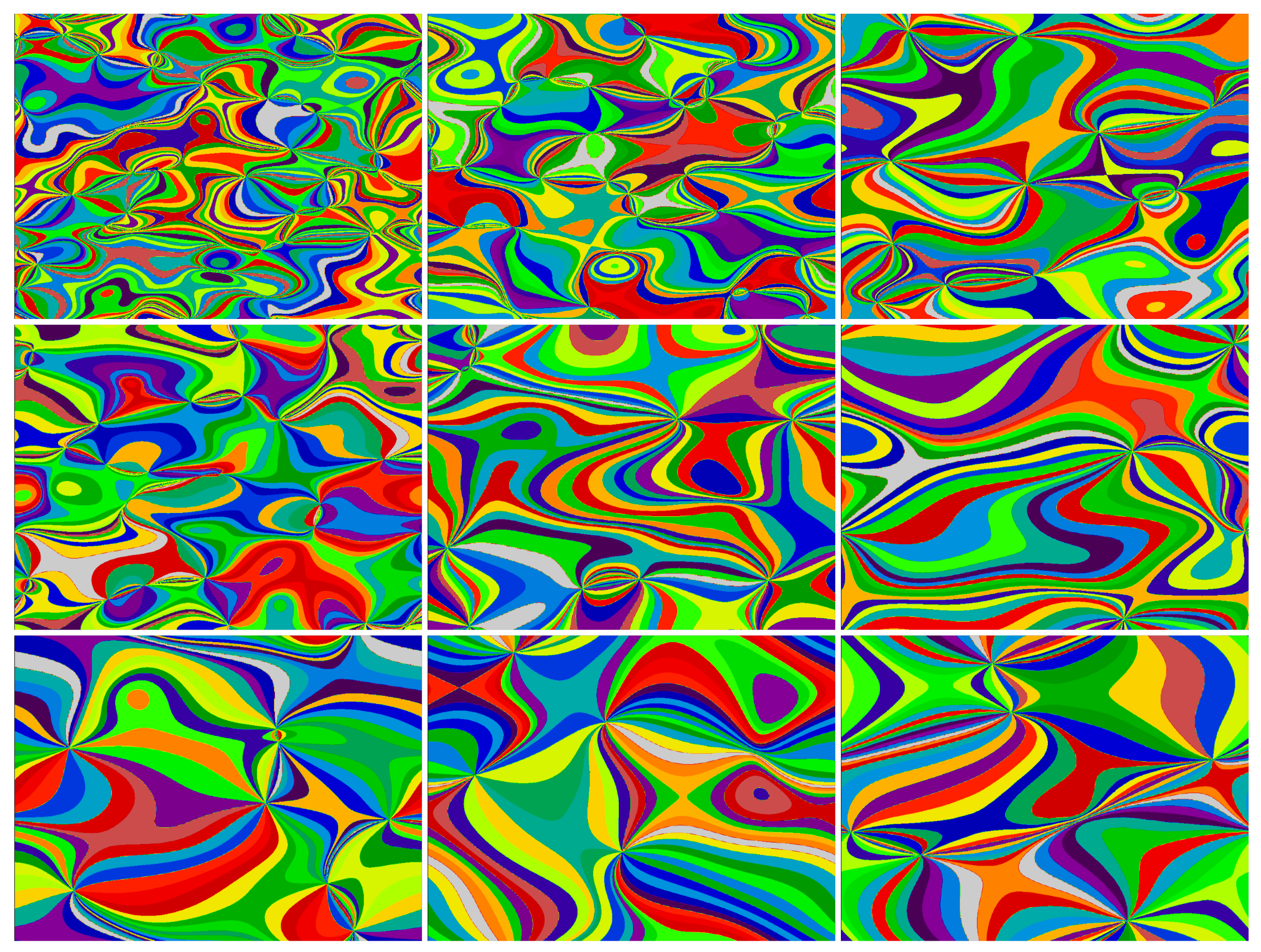
Figure 4.
Examples of binary sampling patterns constructed from a single image map (that map is shown in the top-right subplot of Figure 3). The patterns contain approximately the same number of pixels in the on and off states. In total, we calculate binary sampling patterns, which are then stacked in the measurement matrix . The sampling patterns are projected onto the DMD in the native binary full-resolution mode. The measurement is differential in the sense that only the differences between subsequent intensity measurements are processed, eliminating the influence of background illumination, yet information about the intensity in each region of every image map is guaranteed to be preserved.
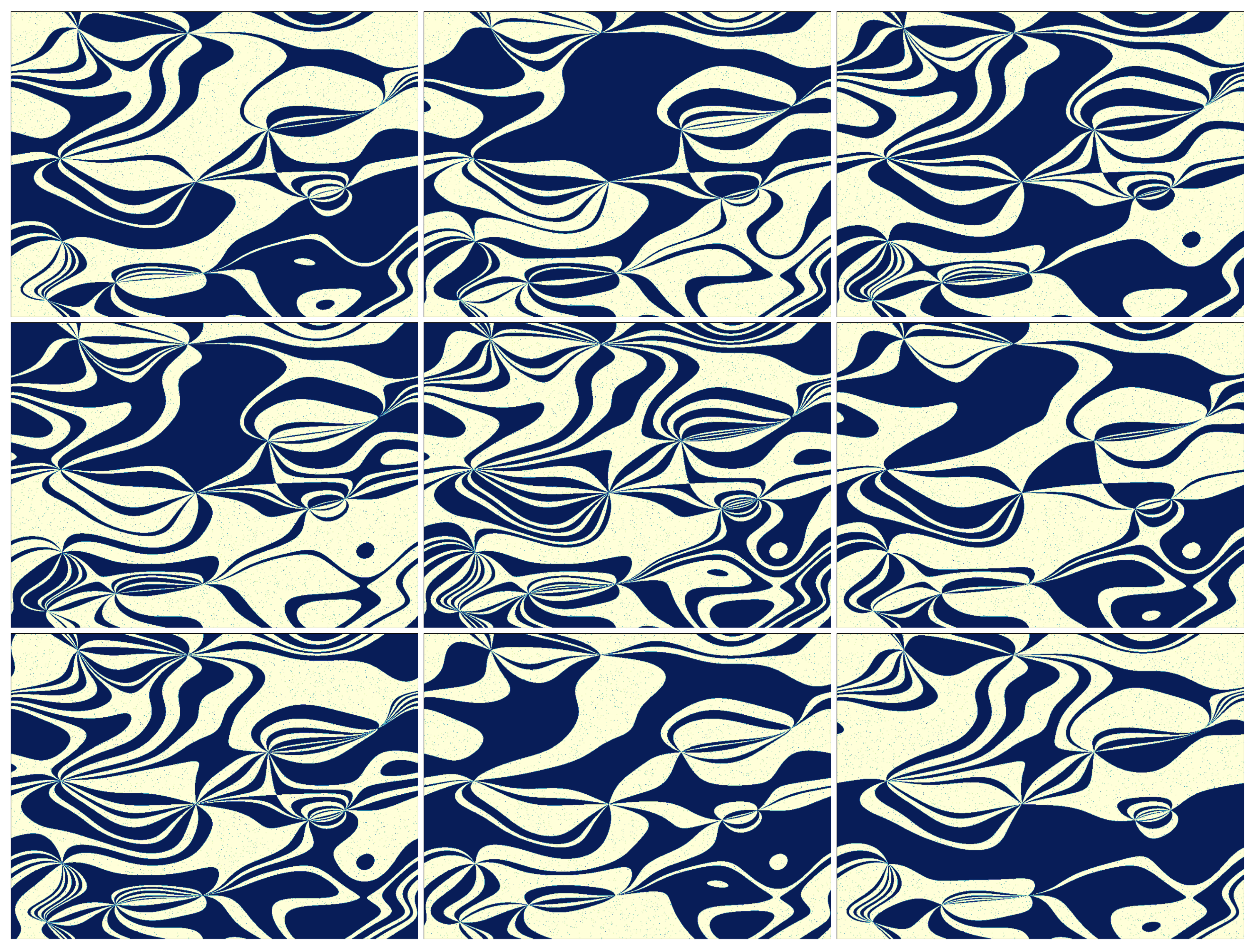
Figure 5.
Graphical representation of the binary lookup table required by Algorithm 1. is a matrix with binary values (here, ) obtained through numerical optimization [31]. Algorithm 1 uses this matrix to construct subsequent rows of the measurement matrix by taking consecutive rows of and treating its columns as an indication of which regions from the map should be included in the sampling pattern.
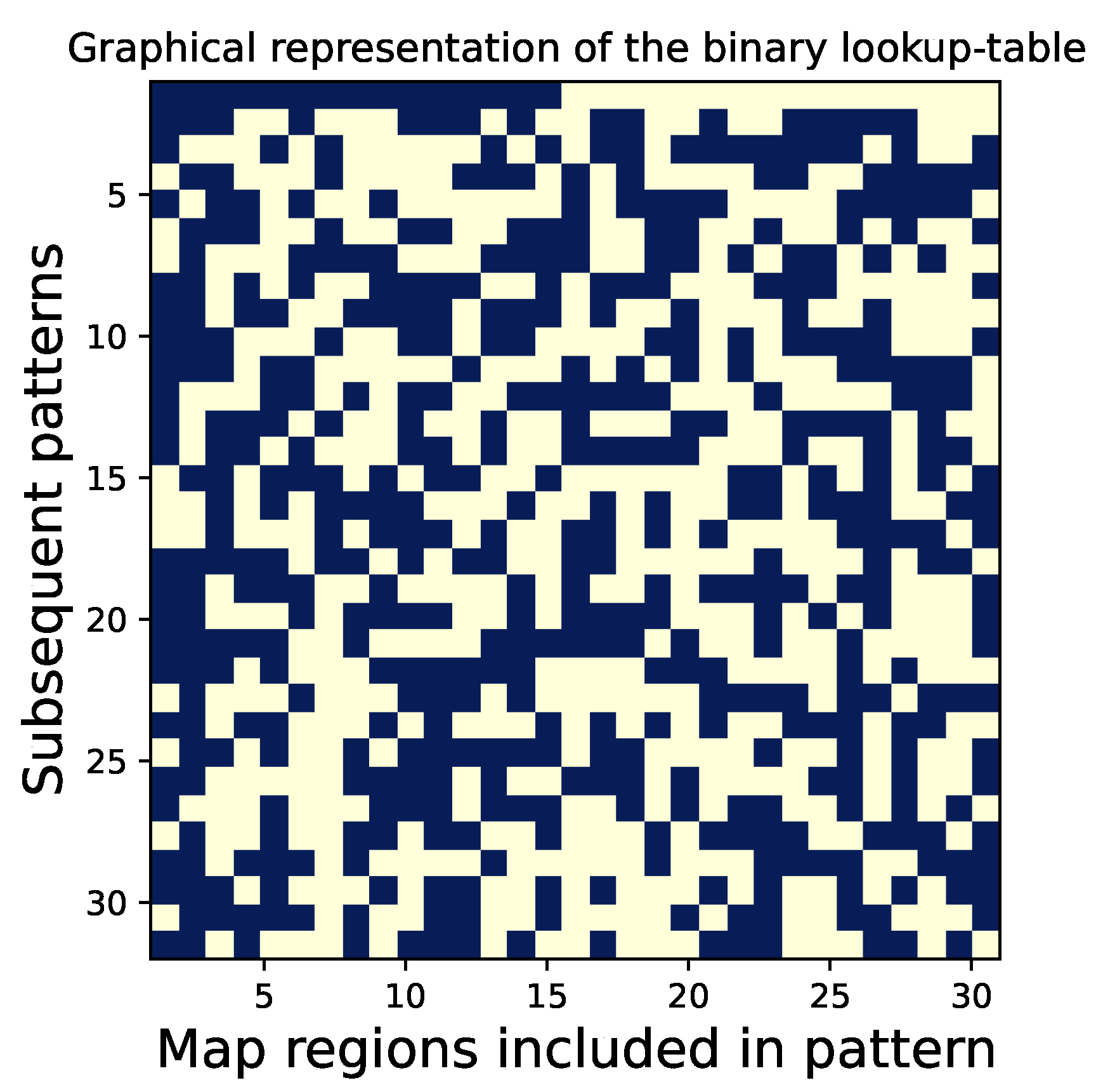
Figure 6.
Examples of binary regions extracted from a single image map (that map is shown in the top-right subplot of Figure 3, and the sampling patterns shown in Figure 4 include superpositions of the binary, non-overlapping regions of the same map). In a mathematical SPI experiment with no necessity of eliminating a DC background bias and with no limiting effect of the small region size on SNR, the binary regions shown in this figure could be used equivalently to the patterns from Figure 4, and both measurements would acquire exactly the same information about the sampled object. In an optical experiment, the patterns from Figure 4 have the advantage of occupying approximately half of the DMD surface and of the inherent possibility of a differential measurement.
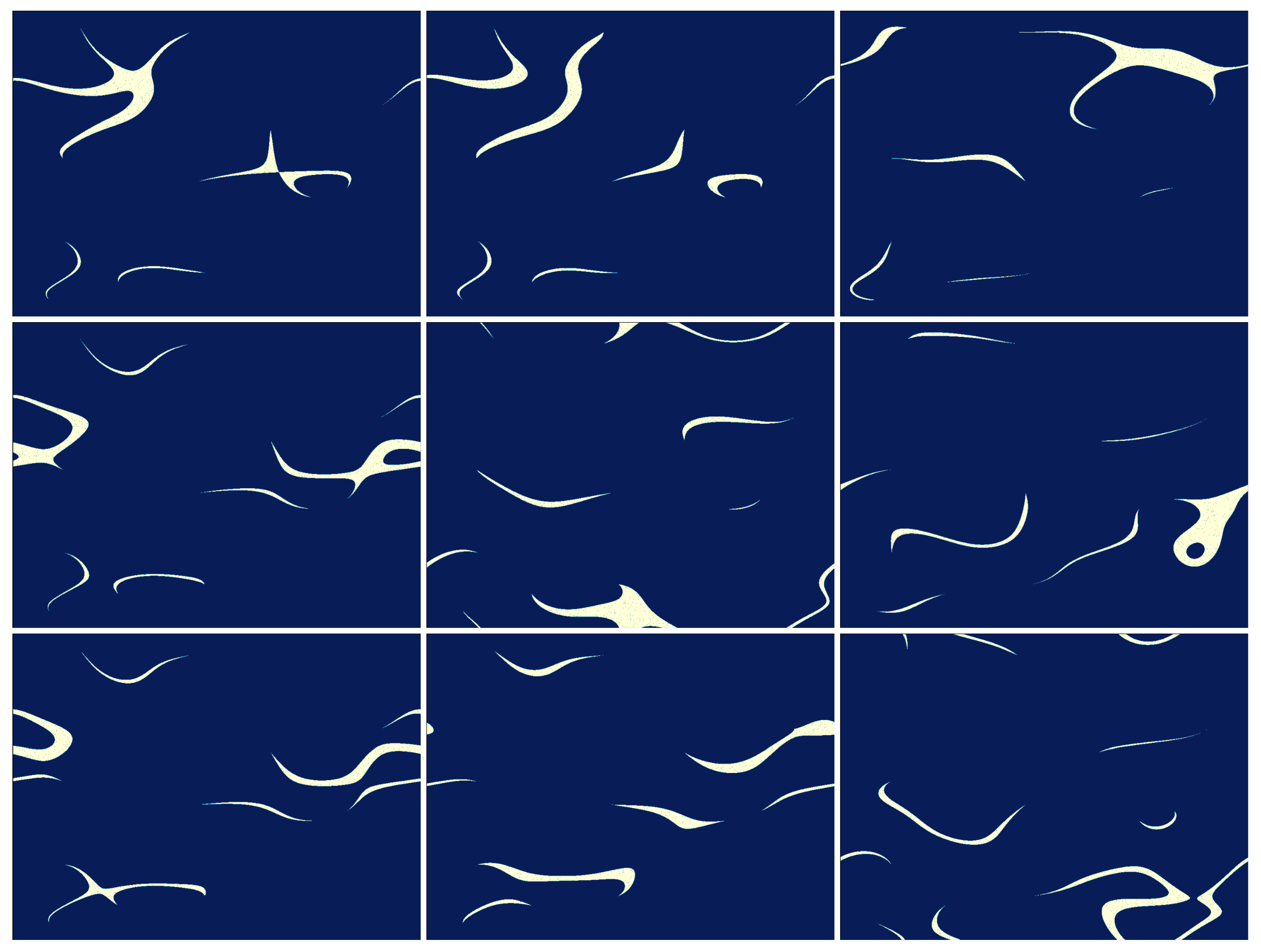
Figure 8.
High-resolution () SPI imaging at very high compression ( %). The three columns show examples of three different types of objects: left — grayscale image (Siemens star) occupying the entire image area, center — grayscale image with a limited support region, and right — binary, high-resolution, highly sparse line art image. The rows, starting from the top, show the ground truth, the SPI measurement data, the first-stage reconstruction result, and the second-stage, improved reconstruction result (50 iterations). The reconstruction quality of sparse images is significantly improved in the second reconstruction stage with Algorithm 2.
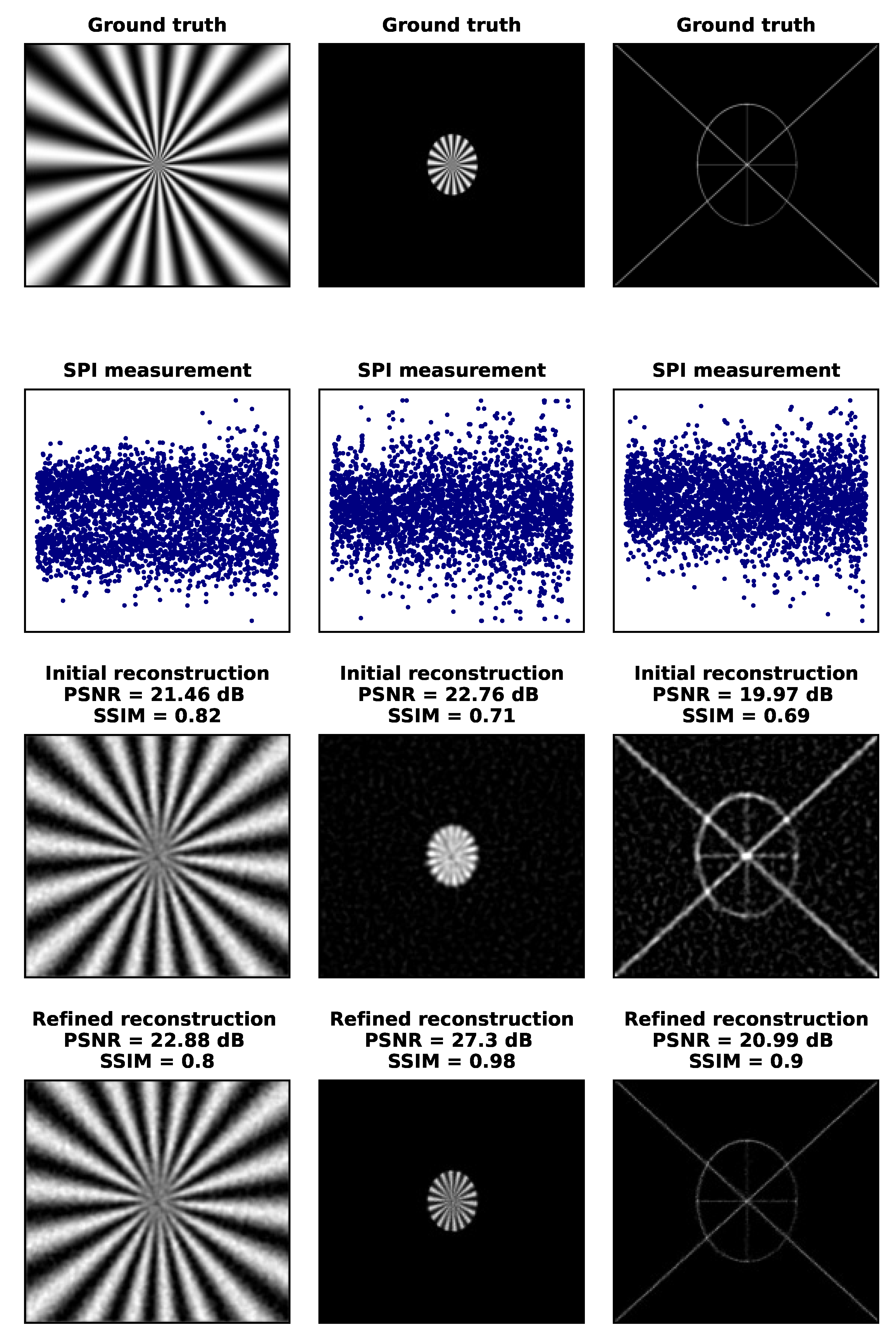
Figure 9.
Convergence of image reconstruction quality in terms of two metrics: (a) PSNR and (b) SSIM as a function of the number of iterations in Algorithm 2. Two variants of the reconstruction algorithm are considered: one with an initial reconstruction calculated using Eq. (4) (wIR), and the other without an initial reconstruction, where the vector is initialized with constant positive values (w/oIR). The performance is evaluated on three distinct images illustrated in Figure 8: a full-area grayscale image (Siemens star), a smaller grayscale image with limited field of view, and a high-resolution, sparse line art image.
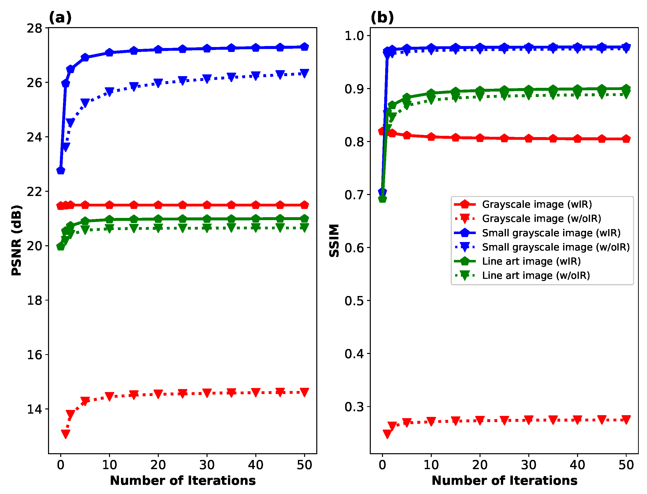
Figure 10.
Performance of Algorithm 2 as a function of bit-resolution of the data acquisition device in terms of two metrics: (a) PSNR and (b) SSIM. The evaluation is performed on three distinct images illustrated in Figure 8: a full-area grayscale image (Siemens star), a smaller grayscale image with limited field of view, and a high-resolution, sparse line art image.
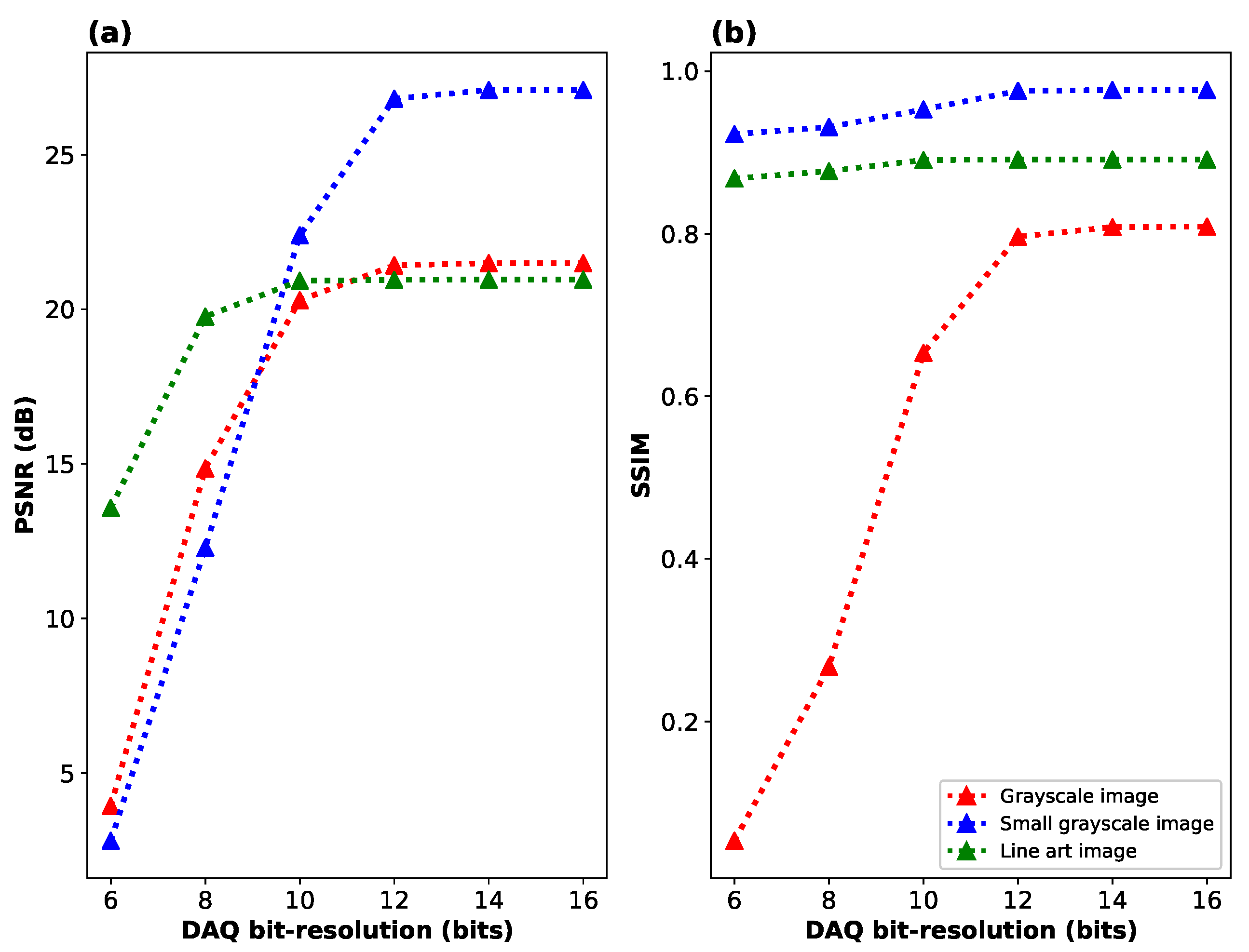
Figure 11.
Examples of image reconstructions obtained using either Algorithm 2 or the neural network as the second stage reconstruction method. In this case, a simulated compressive SPI measurement is performed using several exemplary images from the neural network evaluation dataset as objects. Additive Gaussian detector noise (with =45 dB) is included in the measurement. Columns, starting from the left, display the following: (1) the ground truth images, (2) the initial reconstructions obtained using Eq. (5), (3) reconstructions enhanced with the neural network, and (4) reconstructions enhanced by applying 10 iterations of Algorithm 2.
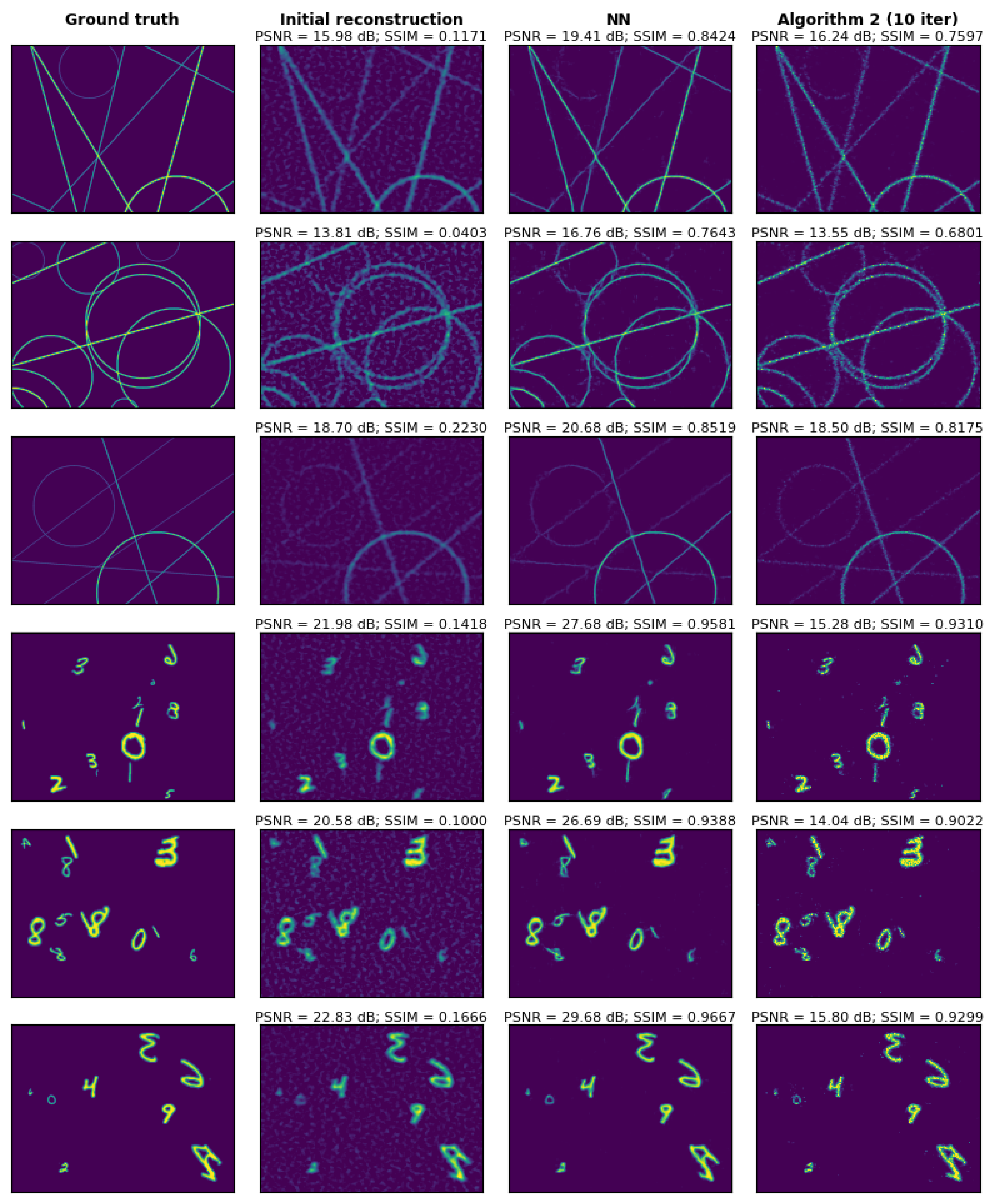
Figure 12.
Sensitivity of the proposed image reconstruction methods to additive SPI measurement noise. We evaluate the quality of the initial reconstructions and the second stage reconstructions, obtained with either Algorithm 2 or the neural network, based on four criteria: (a) the peak signal-to-noise ratio (PSNR), (b) the structural similarity index (SSIM), and (c-d) the optimization criteria and from Eq. (6). The metrics are averaged over a subset of 1,000 images from the evaluation dataset, which consists of an equal mix of line art and handwritten digit images.
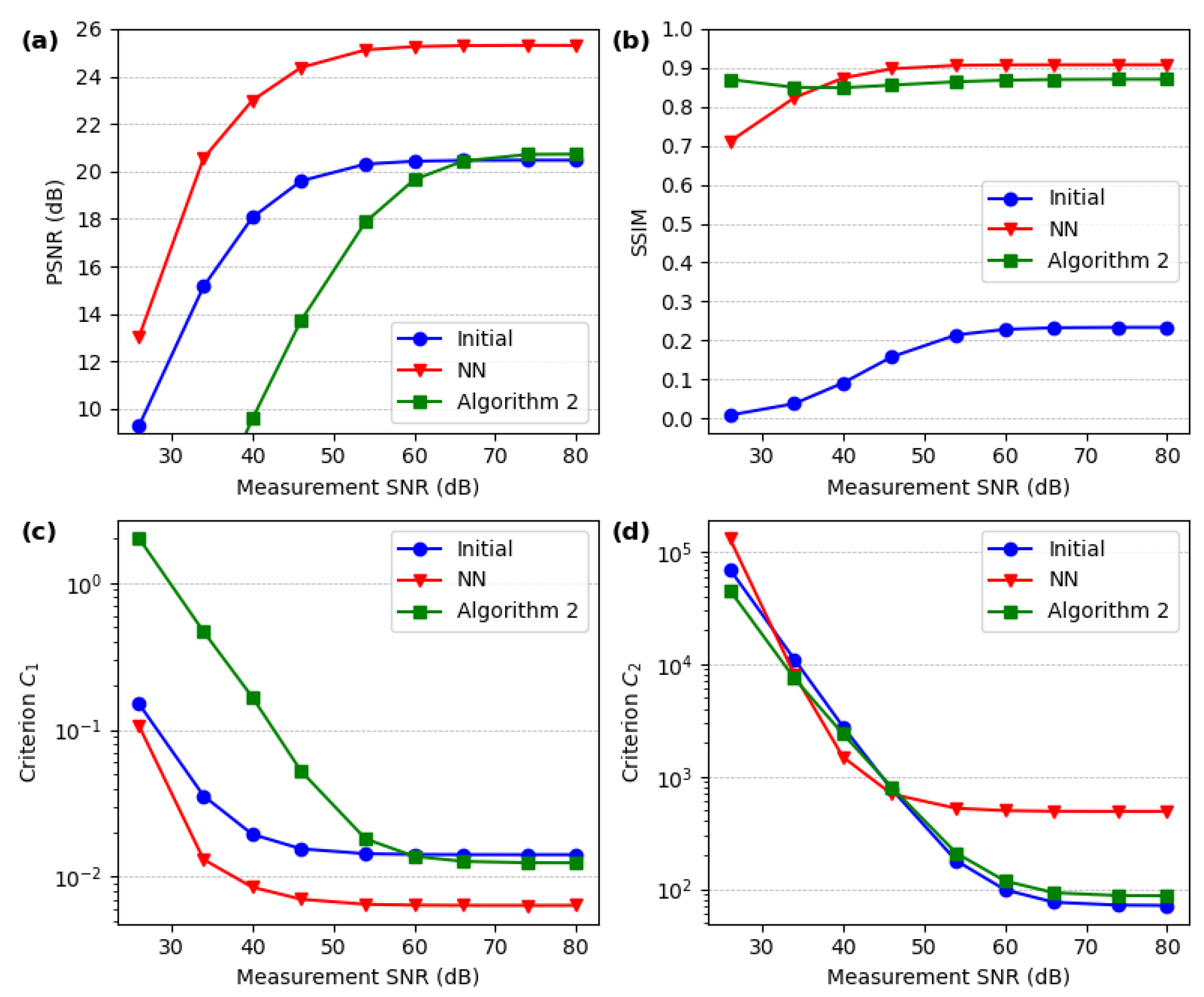
Figure 13.
Experimental high resolution SPI imaging. The object consists of a metal foil with holes arranged in the Faculty of Physics logo of the Univ. of Warsaw. The false colors, red and blue, correspond to the NIR and VIS channels, respectively. The object is static.
Figure 13.
Experimental high resolution SPI imaging. The object consists of a metal foil with holes arranged in the Faculty of Physics logo of the Univ. of Warsaw. The false colors, red and blue, correspond to the NIR and VIS channels, respectively. The object is static.
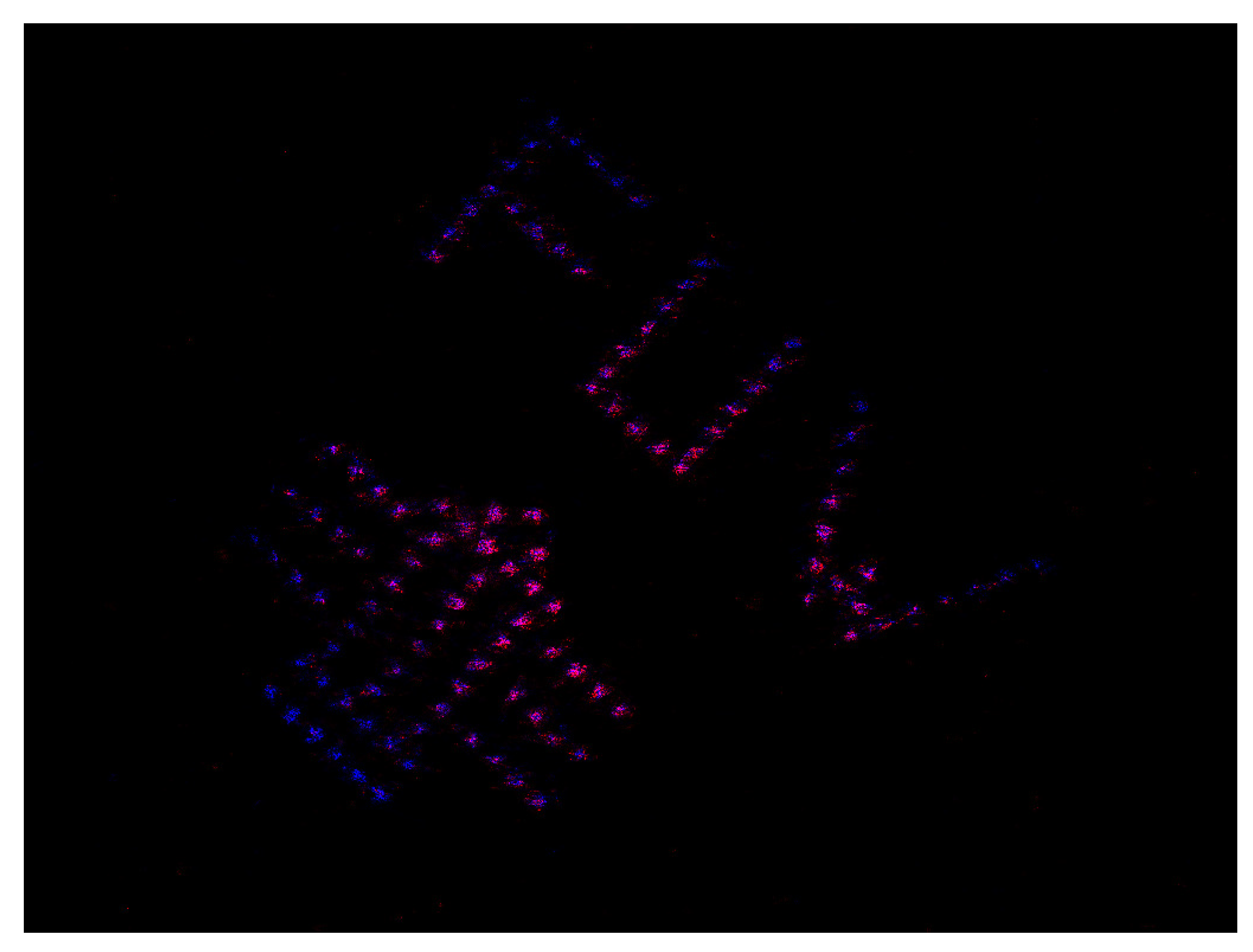
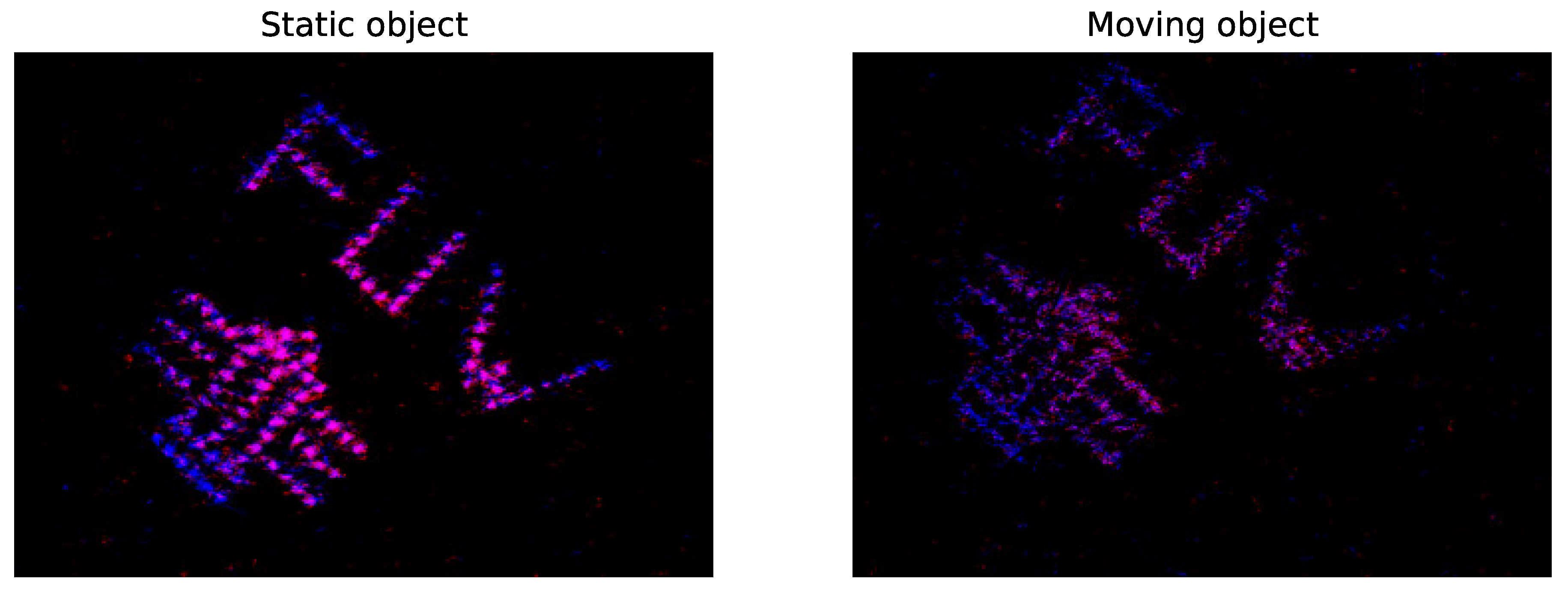
Figure 14.
Experimental high resolution SPI imaging of a static object (left) and of a moving object (right). For better visibility, the contrast of the false color images is enhanced. Object movement during the acquisition of the measurement vector results in deteriorated reconstruction quality and artifacts.
Disclaimer/Publisher’s Note: The statements, opinions and data contained in all publications are solely those of the individual author(s) and contributor(s) and not of MDPI and/or the editor(s). MDPI and/or the editor(s) disclaim responsibility for any injury to people or property resulting from any ideas, methods, instructions or products referred to in the content. |
© 2024 by the authors. Licensee MDPI, Basel, Switzerland. This article is an open access article distributed under the terms and conditions of the Creative Commons Attribution (CC BY) license (http://creativecommons.org/licenses/by/4.0/).
Copyright: This open access article is published under a Creative Commons CC BY 4.0 license, which permit the free download, distribution, and reuse, provided that the author and preprint are cited in any reuse.


