1. Introduction
One of the first methods used in the attempts towards achieving inertial confinement fusion was the Theta Pinch (TP) introduced more than 70 years ago [
1]. Since its conceptualization, many theoretical, numerical simulations and experimental studies were carried out to characterize the temporal and spatial behavior of the plasma in this device [
1,
2,
3,
4,
5,
6,
7,
8,
9,
10,
11,
12,
13,
14,
15,
16,
17,
18,
19,
20]. In the TP configuration, the plasma is generated by ionization of a gas inside a dielectric tube, the result of an azimuthal voltage, induced by a fast-rising high current in an external coil, supplied by a pulse power generator. This induced voltage accelerates background free electrons in the gas to an energy sufficient for impact ionization of gas atoms or molecules. An avalanche is initiated, leading to the formation of a highly ionized plasma sheath in the vicinity of the internal tube surface, where the induced voltage obtains maximal value. A current is induced in the plasma sheath, carried by the electrons, generating a self-magnetic azimuthal field. The interaction of this field with the magnetic field of the current flowing in the coil, leads to a significant magnetic field gradient (magnetic pressure) acting as a piston on the current carrying plasma sheath. This piston creates a shock, propagating inwards toward the axis, while the gas is ionized behind its front. As the main plasma sheath’s radial propagation is accompanied by increasing density and temperature which reach their maximal values in the vicinity of the axis. Earlier research demonstrated that a large electron density plasma, with values exceeding 10
16 cm
-3, and a few hundred eV temperature, forms due to this implosion process [
2].
The most common model describing the TP, and so far best, was introduced by Lee [
8,
12]. This model assumes that a plasma sheath acts as a compressing piston, generating an imploding shockwave which sweeps and ionizes the gas behind its front, a process known as the snow-plow model. The set ordinary differential equations (ODEs) derived by Lee, calculates the shockwave and plasma sheath compression with quite good accuracy accounting for the parameters of the electrical circuit, gas type, and the geometry of the TP. There are two fitting parameters in these equations. The first parameter f is related to the coupling between the circuit and the plasma current while the second parameter f
m describes the fraction of mass being swept by the shock. The time evolution of the loop current and piston and shock front radii are obtained by solving the following ODEs:
where V
0 is the charging voltage of the pulse power supply based on capacitive storage, and C
0, R
0, L
0 are the capacitance, resistance and inductance of the electrical circuit, respectively. I is the discharge current, μ
0 is the vacuum permeability, l
c, r
c are the coil width and radius, respectively. r
p and r
s are the piston and shockwave radii, respectively, γ≈1.67 is the specific heat ratio assuming a fully ionized hydrogen plasma [
21], ρ
0 is the gas initial density and f and f
m are the fitting parameters.
Non-perturbing diagnostics of the plasma generated in the TP, measuring its parameters is crucial. We present the results of experimental studies of plasma generated by a compact Theta Pinch which was designed and assembled in the Plasma Physics and Pulsed Power Laboratory at the Technion. To characterize the TP, several non-perturbing, temporally and spatially resolved, diagnostic methods were employed. These include electrical current and voltage monitors, optical imaging, microwave cut-off, laser interferometry, visible spectroscopy, Thomson scattering, and Laser Induced Fluorescence (LIF) which were applied for the characterization of the plasma dynamics parameters. The main purpose of this study is to explore the applicability of these various, non-perturbing diagnostic methods that will be applied in a much more powerful plasma device being developed at nT-Tao [
22].
2. Experimental Setup and General Parameters of the Theta Pinch
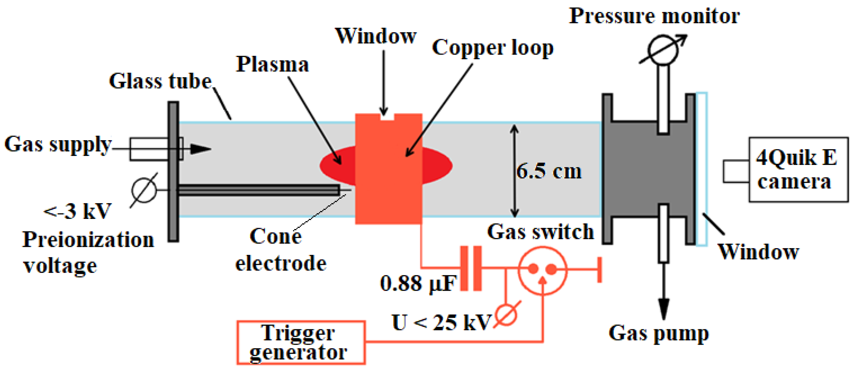
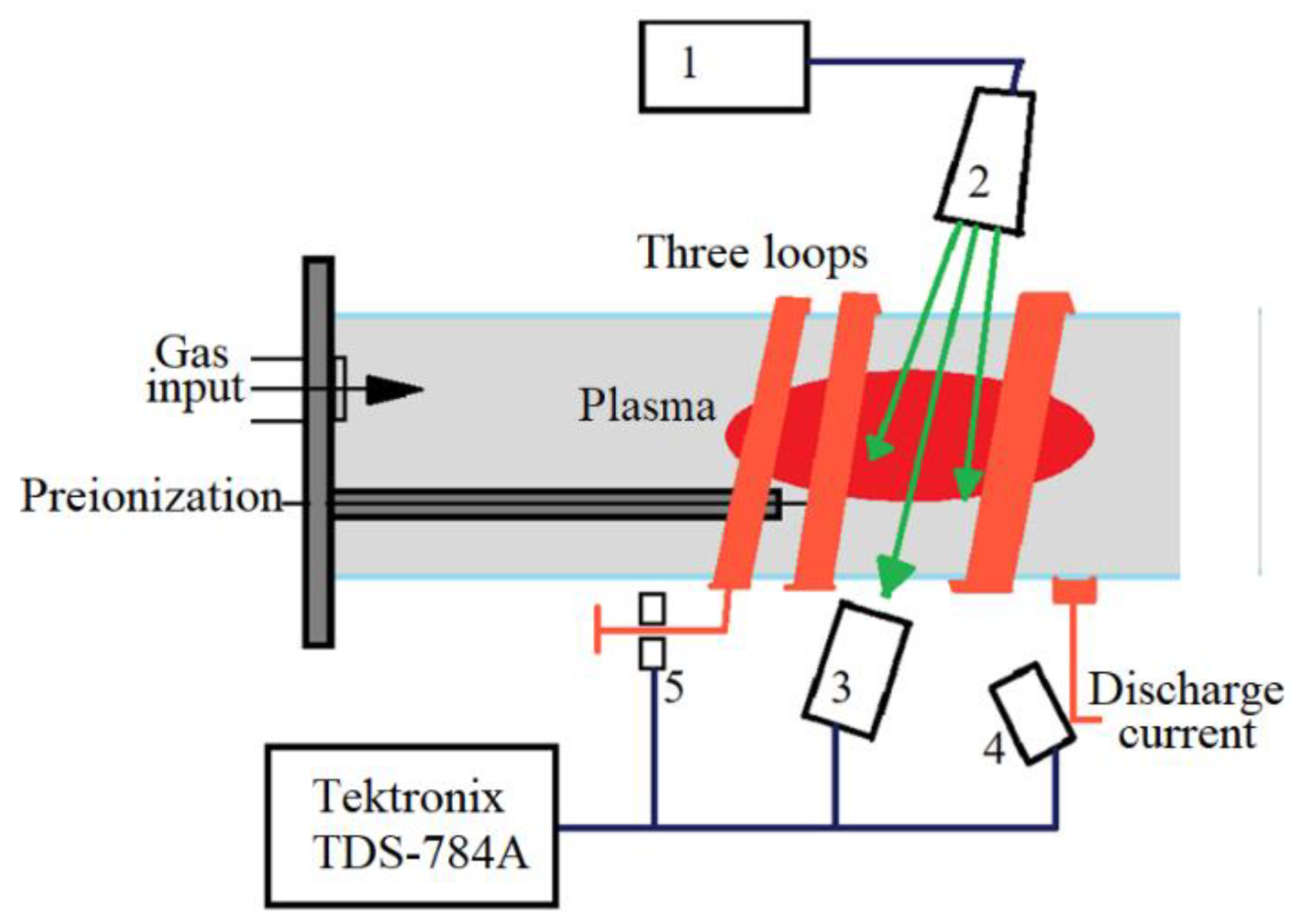
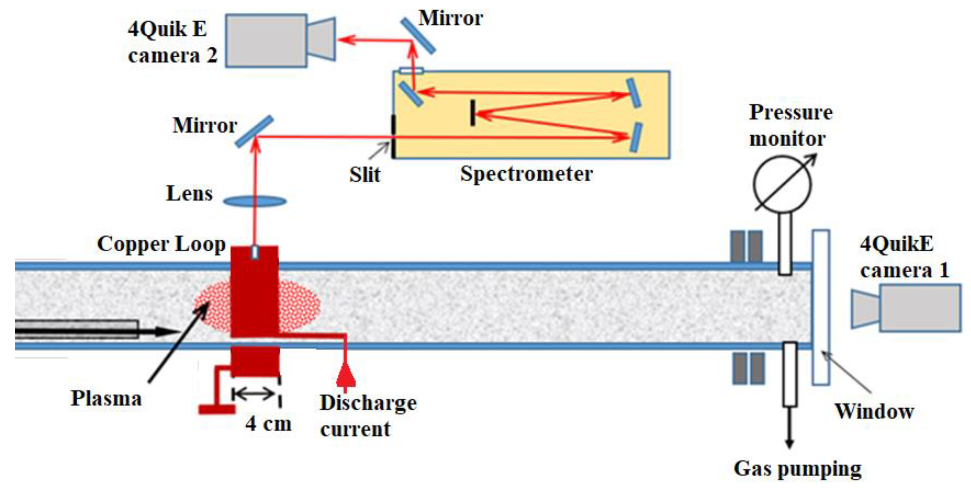
The experimental setup, sketched in
Figure 1, consists of a 65-mm inner diameter Pyrex tube, an induction coil for plasma production and a pulsed power supply. An initial vacuum in the tube of 1 mPa was produced by a turbopump (MacroTorr turbo-V 250) and scroll pump (nXDS15i). The tube is filled with either Hydrogen or Helium gas at a pressure range of 10 -1330 Pa using precise vents and controlled by a baratron gauge (Edwards model 655 AB). 99.99% pure Helium gas is supplied by a gas cylinder. An MRC GG-H-200 generator was used to produce Hydrogen. Continuous pumping and gas injection, keeping constant pressure and using precise gas vents, ensures gas purity in the tube.
For reliable plasma discharge ignition, a sharp cone tungsten electrode was installed in the tube. The electrode is biased to -2 kV pre-ionization voltage supplied by a DC high voltage unit (VC 952 A, Tennelec) via a 2 MΩ resistor connected in series with the electrode. This voltage was sufficient to produce a corona-like discharge which supplies free electrons to the gas filling the tube volume.
Characterization of the plasma using microwave cut-off and laser interferometry were carried out with a 3-loop coil (0.5-mm thick, 20-mm wide copper foil) wrapped around the glass tube. The advantage of a 3-loop coil is that given an equal dI/dt of the discharge current, a larger magnetic field flux, Φ3 , is generated compared to the magnetic field flux, Φ1 , enerated by a single loop. Thus, the 3-loop coil generates a larger induced voltage, ε3, than that induced by a single loop coil, ε1, as: where Lg and L1 are the inductances of the pulse generator and that of a single coil, respectively.
Although a 3-loop coil can produce a larger induced voltage (when the condition Lg>>L1 is satisfied), the plasma forms with spatial non-uniformities across the tube due to the discrete number of turns, having, in the present setup, gaps of ~2 cm. Therefore, in experiments involving fast framing imaging of the plasma light emission, spectroscopy, Thomson scattering and LIF, we used a setup with only a single turn of 0.5-mm thick and 40-mm wide copper foil.
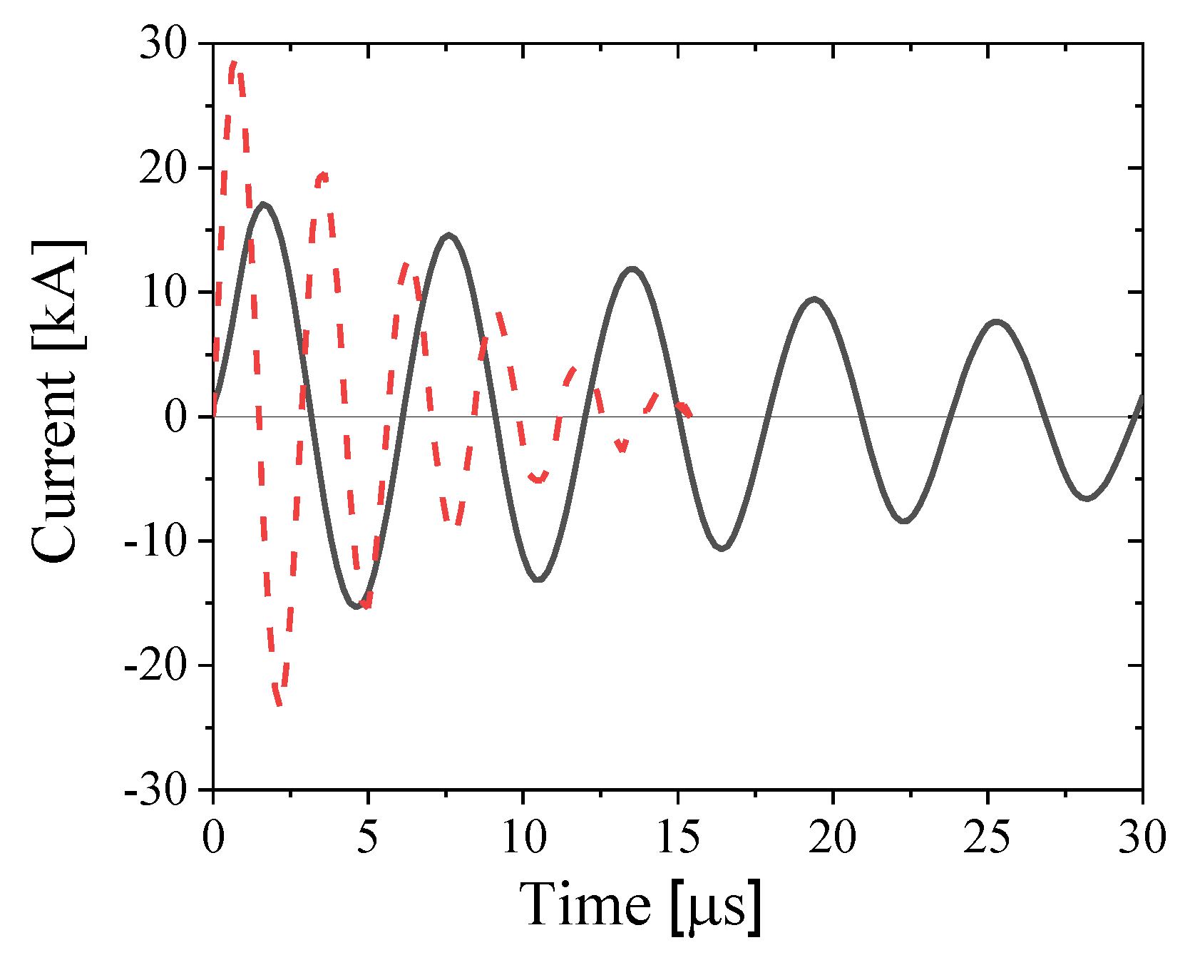
Two pulse power, high-current, generators were applied in this research for the generation of a TP plasma. A Fluke, 40 kV DC voltage divider, was used to control the charging voltage of the generators, and a Pierson current monitor (model 5046) was used to measure the discharge current the waveform of which was registered by a Tektronix TDS-784A (1 GHz, 4 Gs/s) oscilloscope. The generator used for the 3-loop coil setup, consisted of a low-inductance 1 μF, 20 kV capacitor (Condenser Products Corp.) charged to 17 kV (stored energy of ~145 J) discharged using a gas spark gap switch with an externally triggered middle distortion electrode. A typical waveform of the discharge current obtained at He gas pressure of 0.1 Pa when a plasma discharge does not develop, is shown in
Figure 2. The discharge current is characterized by ~1.5 μs rise time reaching an amplitude of I = 17.5 kA and dI⁄dt ≈ 1.1×10
10 A/s. However, due to an underdamped discharge, characterized by current oscillations with a ~34.8 μs decay, the lifetime of this capacitor was limited to several hundreds of shots. A second generator, based on two 0.44 μF, 50 kV, 20 nF capacitors (General Atomics) connected in parallel, operated at 25 kV charging voltage (stored energy of 275 J) which is smaller than its nominal value by a factor of two. This generator was used in experiments with a single loop coil (see
Figure 1). For this case, a 0.7 μs rise time, ~29 kA amplitude discharge current (see
Figure 2) with dI⁄dt ≈ 4.1×10
10 A/s was obtained with a fast ~7 μs decay time (see
Figure 2). Using the decay of the discharge current oscillations, we calculated the impedance, inductance and resistance of the 3-loop and single loop setups as ~0.93 Ω, ~0.95 μH, ~17 mΩ and ~0.7 Ω, ~0.56 μH and ~14 m Ω respectively.
As a result of the fast discharge, a longitudinal oscillating magnetic field is generated in the tube which, in turn, induces an azimuthal electric field. Estimating the electric field in the vicinity of the loop as , where is the inductance of a coil with N loops, of (loop radius) and foil width. These estimates give ~40.5 V/cm and ~50.4 V/cm for the 3-loop and single loop setups, respectively. These electric fields accelerate free electrons, which acquire sufficient energy for gas ionization, resulting in an avalanche and a current carrying plasma sheath. The interaction of the induced magnetic field created by the plasma current with the external magnetic field of the current in the coil, leads to a magnetic field gradient which compresses the plasma. Thus, the energy of the time-dependent magnetic field, created by the current flowing in the loop, is transferred into ionization and excitation of the gas and radial compression of the plasma sheath.
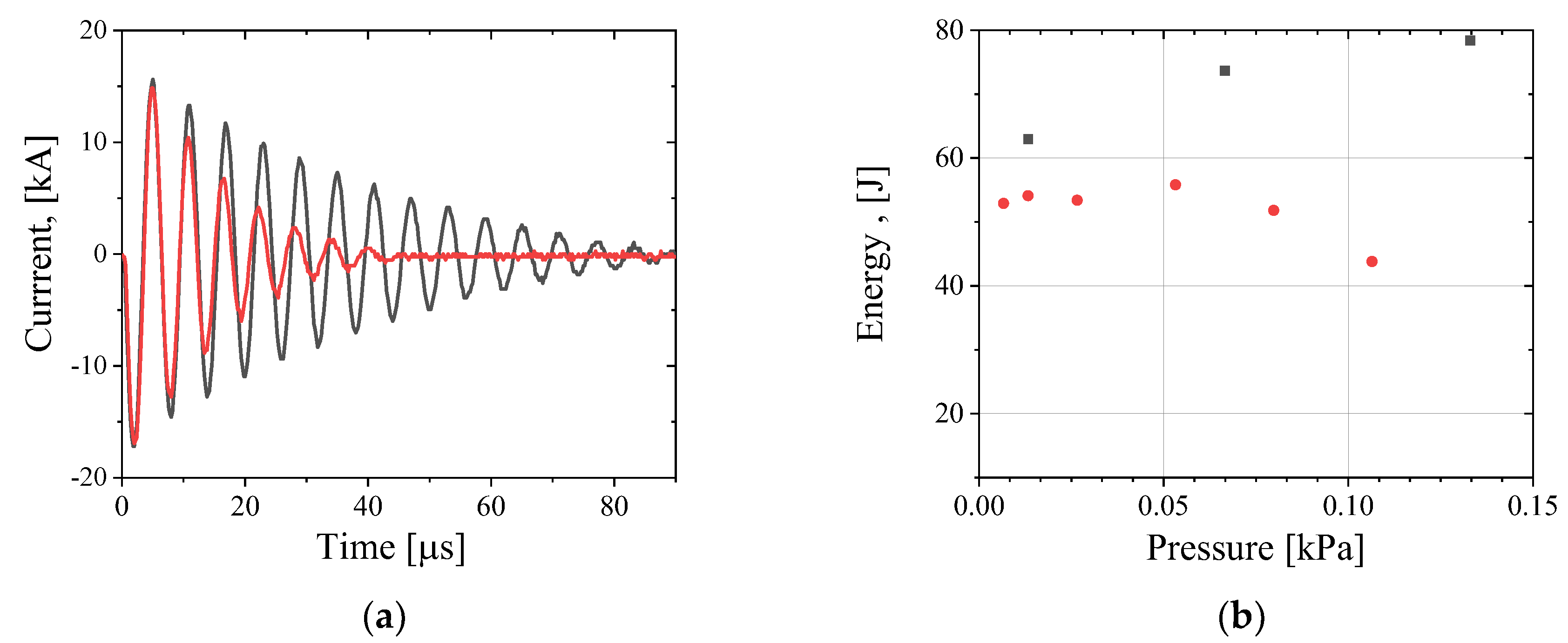
In
Figure 3(
a) we present waveforms of the discharge current in a 3-loop coil obtained with He gas at P = 2.7 kPa and at P = 0.4 kPa. For the higher pressure, plasma formation was not obtained. When plasma forms, a much faster decay of the discharge current is observed due to energy transfer to the gas ionization and plasma compression. In
Figure 3(
b) we present dependencies of the energy transfer to Helium and Hydrogen plasmas as function of pressure.
For He plasma, up to 55 % of the stored energy was transferred to the plasma while for Hydrogen plasma ≤ 38 %. Here, the energy transferred to the plasma was calculated as the time integrated power, , subtracted from the total energy initially stored in the capacitor. The resistance R was calculated using the decay constant of the discharge current .
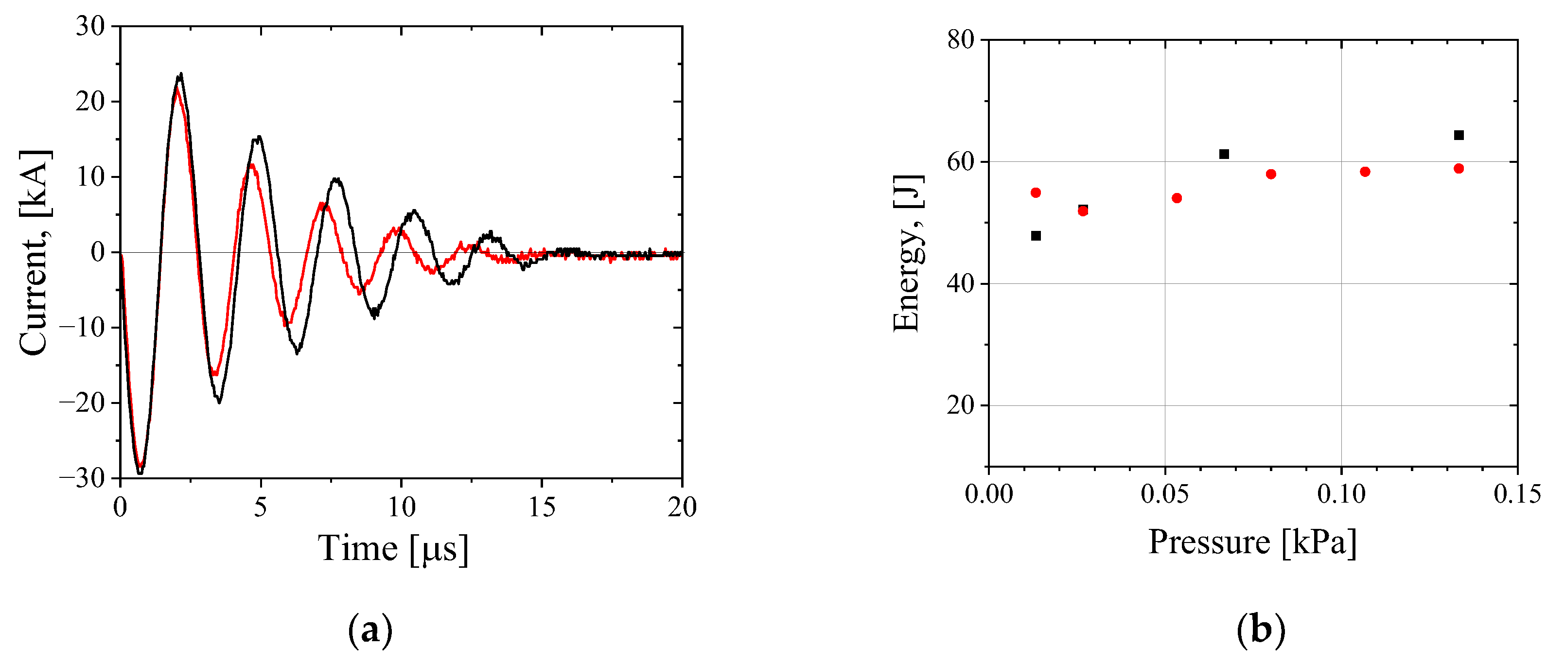
In
Figure 4(
a) we present waveforms like those shown in Fig. 3 but obtained with a single loop at 0.1 Pa and 0.4 kPa of He gas pressure. As in the 3-loop scheme, when plasma generation occurs, current oscillations decay faster.
Figure 4(
b) presents the stored energy transfer to the plasma for different gas pressures. The efficiency of the energy transfer to the plasma is smaller than those obtained for the 3-loop scheme. This can be explained by the smaller period of the current oscillations, meaning that the time for energy transfer to the plasma during its compression was not sufficient.
3. Experimental Results
3.1. Time and Space Resolved Light Emission During Plasma Compression
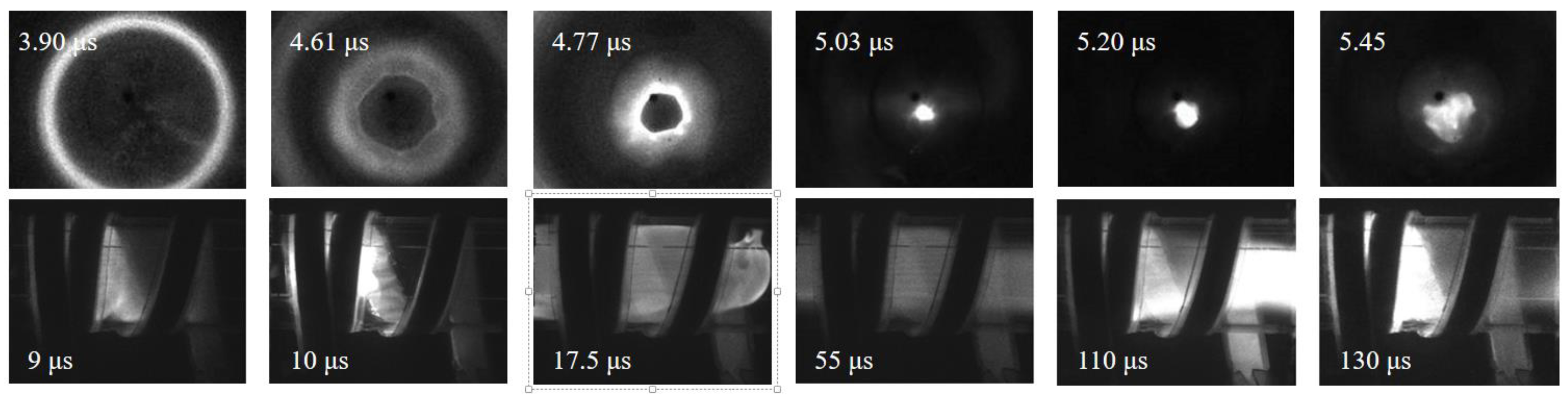
In
Figure 5 we show an example of Hydrogen plasma light emission images obtained by a 4QuikE intensified camera (Stanford Computer Optics) during plasma compression at P = 63 Pa. In experiments with a single loop, the 4QuikE camera was installed in front of the glass tube along its axis, with its focus set to the center of the loop (see
Figure 1). The images presented in the upper row of
Figure 5 reveal that the bright light emission from the plasma is obtained at the periphery of the tube, approximately half a period after the beginning of the discharge current and plasma compression takes ~
. This time is estimated when the spatial size of the plasma emission pattern reaches its smallest value (~5 mm). The latter allows to estimate the average implosion velocity of the plasma as
at 63 Pa gas pressure for both Hydrogen and Helium. Side view images obtained for the 3-loop coil setup (see the images in the bottom row of
Figure 5), show non uniform plasma formation along the width of the loops. Additionally, the plasma is compressed to a larger final radius compared to the single loop experiments.
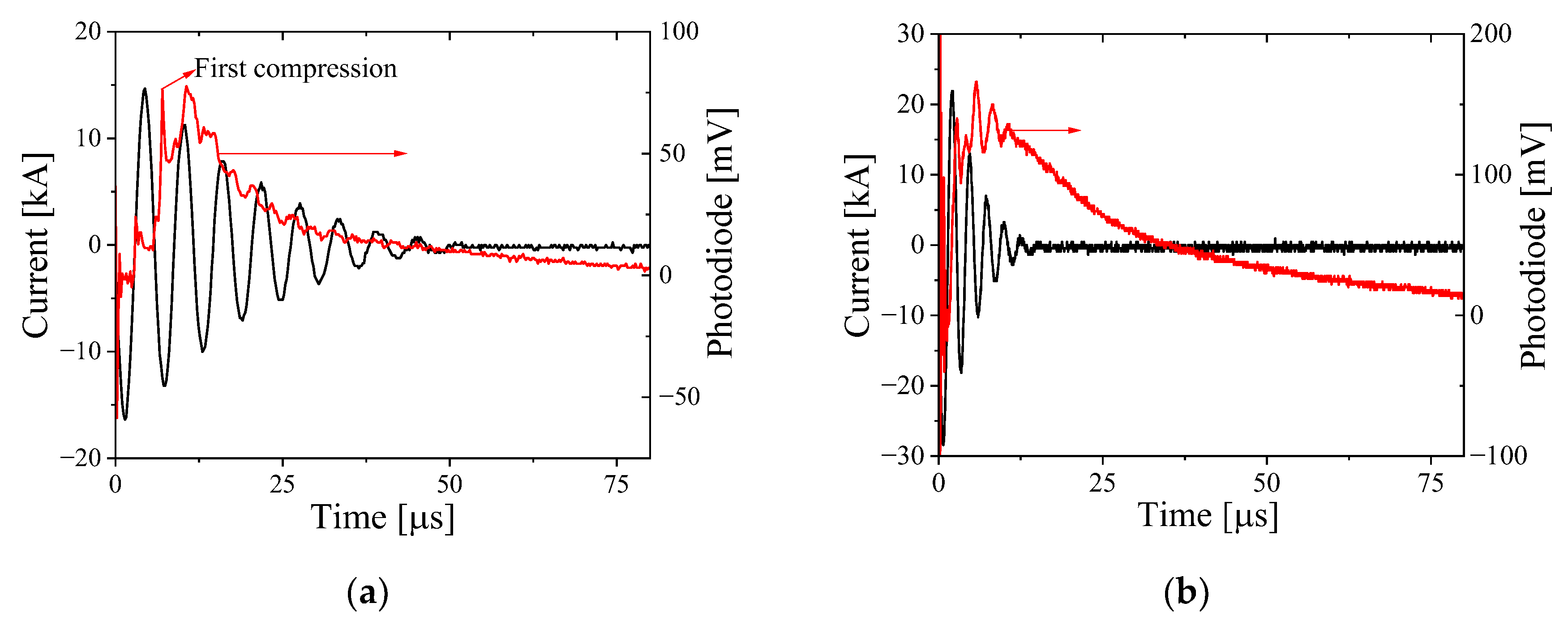
We used a fast photodiode (DET02AFC, Thorlabs) to obtain the time evolution of the light emission from the plasma. In the photodiode data (see
Figure 6) compression is seen as the fast-rising intensity and the quality of compression can be estimated by the duration and amplitude of the first peak in the light intensity. A light emission from the plasma was obtained over 80 µs, giving an estimated plasma lifetime.
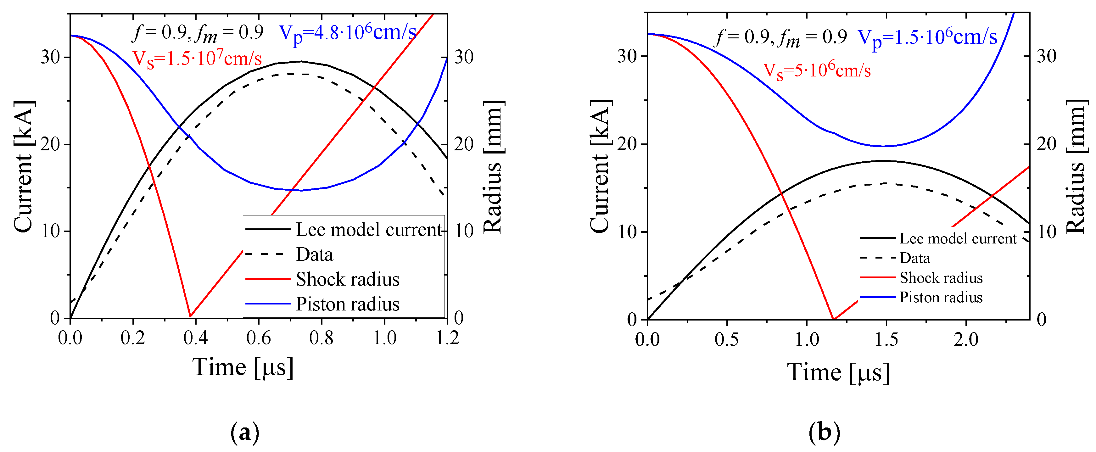
In
Figure 7 we present the results of numerical simulations using the Lee model for the 3-loop and single loop setups. The simulated current waveform shows satisfactory agreement with the measured current for fitting parameter values of
. Numerically calculated shock and piston radii show maximum implosion velocities of ~1.5×10
7 cm/s and ~4.8×10
6 cm/s, respectively for a single loop. This result agrees satisfactorily with the average velocity of the plasma implosion obtained using the framing images of the plasma light intensity. For the 3-loop setup, these velocities are ~5×10
6 cm/s and ~1.5×10
6 cm/s.
3.2. Microwave Cut-Off Measurements
Propagation of electromagnetic (EM) waves in the plasma in the absence of magnetic field, is possible only when the frequency of the EM waves is higher than the plasma electron frequency, where is the plasma electron density, e the electron charge, the electron mass and the vacuum permittivity. Here it is assumed that where is the electron-neutral collision frequency. This can be used to obtain the lifetime of a plasma with a density larger than the critical density:
In the present research a klystron (model 44151H, Hughes EDD) was used as a 70 GHz continuous wave (CW) microwave source. The klystron was connected to a WR15 waveguide (50 – 75 GHz) with an ANTT-SGH-50-70 horn antenna (gain of 24.4 dBi) at its output. The antenna was located at a distance of 3 cm from the 3-loop setup and positioned between the space between the loops, allowing microwaves to pass through the tube wall (see
Figure 8). On the opposite side of the tube, a receiving NTT-SGH-50-70 antenna was placed at the same distance of 3 cm from the tube. This antenna was coupled with a coaxial adapter and the microwave signal was detected by a Schottky diode. In these experiments a fast photodiode was used to provide the dynamics of light emission from the plasma.
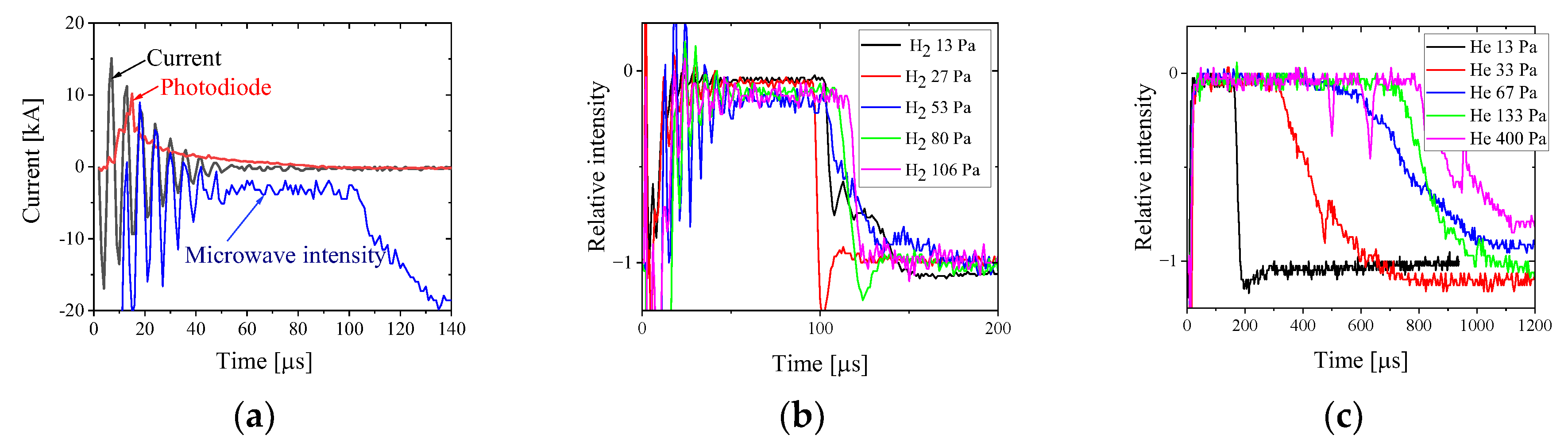
Using this setup, the lifetime of the plasma with
corresponding to
was studied for Helium and Hydrogen plasmas, generated by the TP for different gas pressures. Examples of these measurements are shown in
Figure 9. A plasma with electron density
exists for ~100 µs and up to ~800 µs for Hydrogen and Helium plasmas, respectively. Moreover, increasing gas pressure leads to an increase in the plasma lifetime.
3.3. Laser Interferometry
Since the microwave cut-off experiments only provide the lifetime of a plasma with
, laser interferometry was implemented to study the time-resolved line-integrated plasma density evolution across the tube’s diameter. Laser interferometry is based on the phase shift acquired by a laser beam propagating through plasma, with respect to a reference laser beam propagating in air. The phase shift can be calculated as:
where
is the frequency of the laser beam,
is the plasma length, c is the speed of light,
is the phase shift related to the difference in two arms of the interferometer due to vibration of the optical elements, and
is the dielectric constant of the plasma [
23]:
Thus, the plasma electron density can be calculated in terms of the phase shift as:
where λ is the laser wavelength.
In the experiment, when two waves
are added at one point in space (at the input of the fast photodiode), the resulting wave intensity is
. In our case, the phase shift accounting for the acoustic vibration of the optical elements is equal to
Therefore we use two digitizing oscilloscopes with data acquisition with two different time sweeps. The phase shift for the measured signals can be found as:
where
and
obtained from the waveform registered by the digitizing oscilloscope with the slow timescale. Here
and
are the maximum and minimum amplitudes of slow interference signal during plasma generation. Thus, the phase shift
is given as:
We used an in-house MATLAB code for signal processing which includes FFT filtering of the noise and signal smoothing procedures.
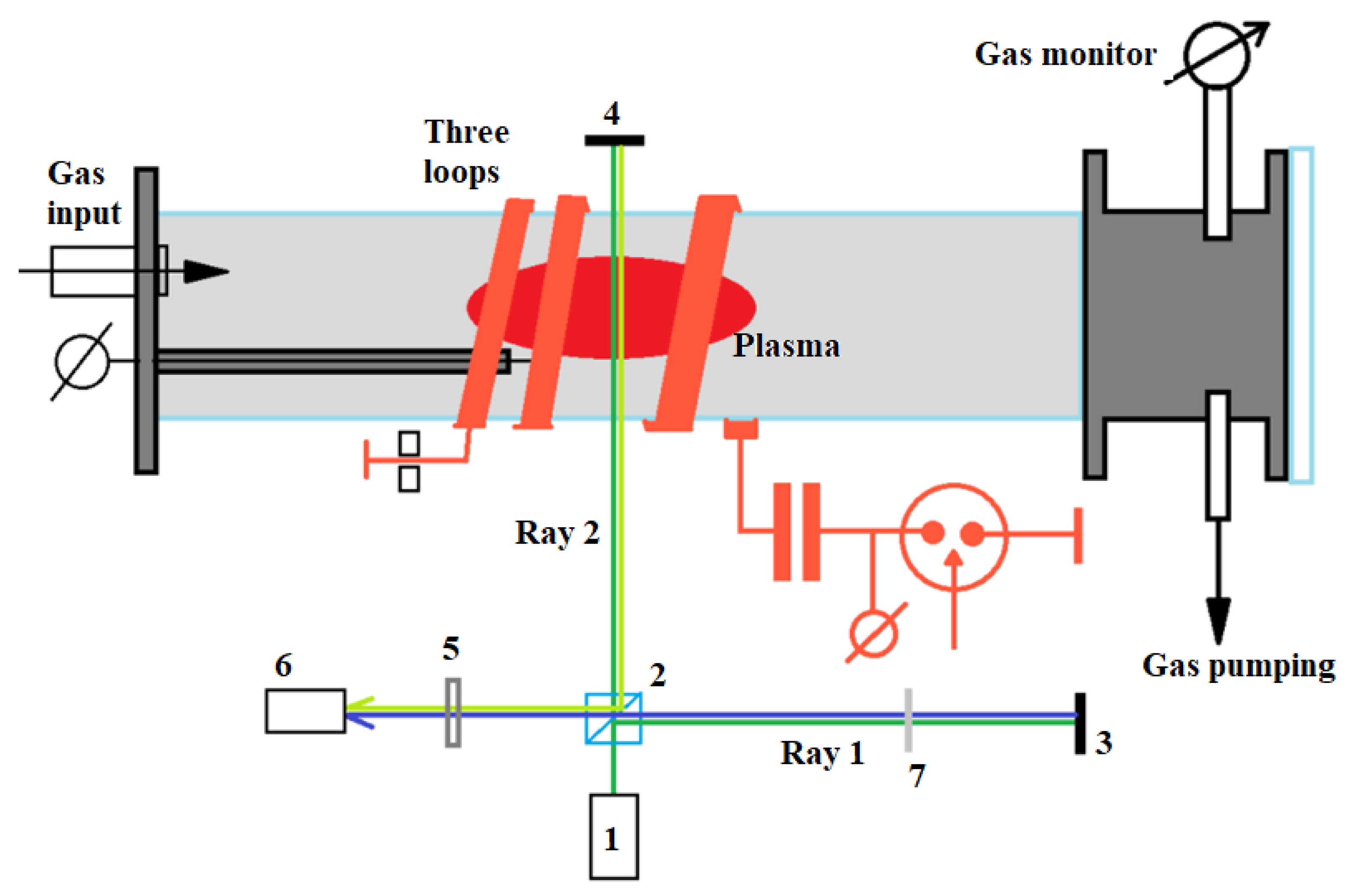
In this set of experiments, a Michelson interferometer was assembled (see
Figure 10). The interferometer consists of either a red laser (λ = 632.8 nm, P = 15 mW) or a green laser (λ = 532 nm, P = 200 mW) (1), beam splitter (2), two mirrors (3,4), ND filter 0.3 (7), bandpass filter (λ=632±1 nm or 530±5 nm) (5) and a fast photodiode FDS010 ThorLabs (1 ns time resolution) (6). A laser beam is split between mirrors (3) and (4) using a beam splitter. One of the beams propagates through a Pyrex tube where the plasma is generated. The reflected laser beams (Ray 1 and Ray 2) from mirrors (3) and (4) are returned and combined by the beam splitter and are registered by a fast photodiode. Ray 2 has a phase shift relative to Ray 1 due to a change in the plasma density, resulting in an interference signal at the diode output.
Waveforms of the voltage from the fast photodiode (6) are registered by two digitizing oscilloscopes: Tektronix TDS-2014C and Tektronix TDS-784A. The Tektronix TDS-2014C acquires a signal with a slow time sweep (250 - 2500 μs/div) and the Tektronix TDS-784A with a faster time sweep (20-50 μs/div). Thus, we obtain an interference waveform due to low-frequency vibration of optical objects (mirrors, etc.) using the Tektronix TDS-2014C oscilloscope. The signal from the photodiode which collects the plasma light, allows us to obtain an initial maximal and minimal amplitudes of the interference signal which appears due to acoustic motion of mirrors at the time of the plasma density evolution.
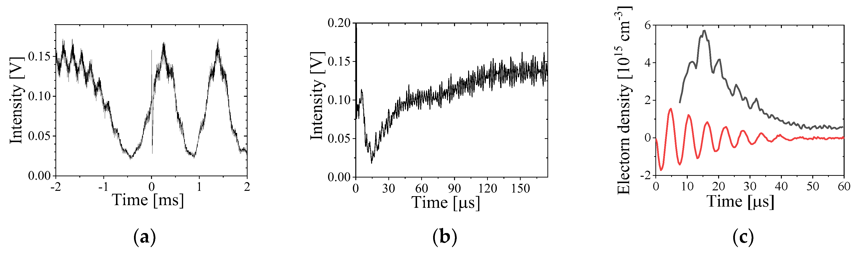
Interference waveforms measured in a single shot with the two oscilloscopes on the ms and μs timescales are shown in
Figure 11(
a) and
Figure 11(
b). On the ms timescale, low frequency oscillations are seen due to acoustic motion of the mirrors. These provide the interference amplitude and phase difference over the plasma density’s evolution time. On the μs timescale, with plasma formation, a change in the amplitude of the interference signal, caused by the phase shift of Ray 2, is registered. This effect happens due to the plasma’s rising dielectric index due to its density increase. Results for 53 Pa Hydrogen plasma density for the 3-loop setup are shown in
Figure 11 (
c).
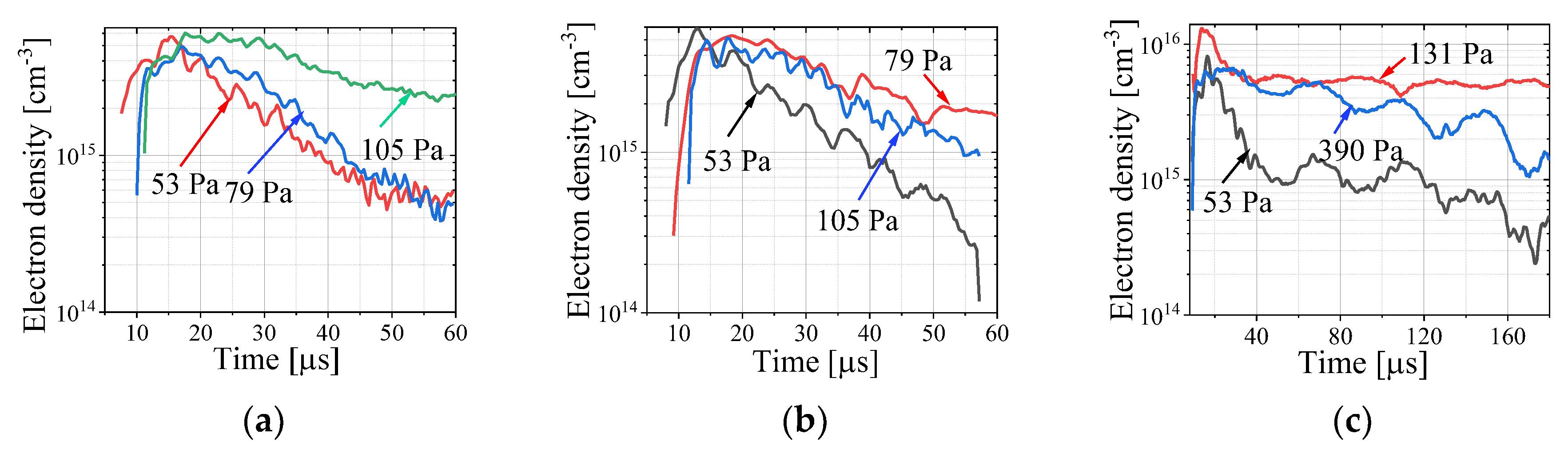
In
Figure 12 we present the results of the average electron density evolution in Hydrogen and Helium plasmas. For Hydrogen, the maximal plasma density increases up to 6×10
15 cm
-3 in the pressure range of 53-105 Pa, respectively. Additionally, the increase in pressure leads to a slower decay in the plasma density. Furthermore, the results obtained using green (see
Figure 12 (
a)) and red (see
Figure 12(
b)] lasers agree quite well. For a Helium plasma, the maximal electron density of ~10
16 cm
-3 was estimated at 131 Pa [see
Figure 12(
c)]. Here we emphasize again, that this method gives the line integrated plasma density averaged along the length of the laser propagation, resulting in a significantly larger plasma density at the time when the implosion is expected.
3.4. Results of Visible Spectroscopy
Plasma spectroscopy utilizes high resolution spectral line measurements of the emitted plasma light by which the plasma density and temperature can be estimated. Here (see
Figure 13), the light emitted from the plasma was collected by a 100-mm diameter lens and focused (170-mm focal length) onto a 100-µm wide slit of a 1 m long focus spectrometer with a grating of 2400 grooves/mm. At the output of the spectrometer a fast-framing 4QuikE intensified camera was installed (see
Figure 13). To obtain reliable spectral line profiles, the duration of the camera frame in these experiments was 100 ns. Thus, the density and temperature obtained by analyzing the spectral lines should be considered as an average value during the exposure time. Spectral lines were obtained at various times relative to the beginning of the discharge current by controlling the time delay of the camera’s trigger time. Spectral calibration of the spectrometer at Hα (656.28 nm) and Hβ (486.13nm) spectral lines using Hydrogen spectral lamps resulted in
and
Using this spectral resolution, the instrumental Full Width at Half Maximum (FWHM) broadening of Hα and Hβ spectral lines was found to be
and
.
For a Hydrogen plasma, the main effects responsible for line broadening are Doppler broadenings due to Hydrogen atom temperatures and Stark broadening created by the electric fields of the electrons and ions. To distinguish between the contributions of these two effects, the following algorithm was applied. The
line Stark broadening is smaller than the
line Stark broadening for the same density of the plasma [
23]. However, the Doppler broadening of the
line is larger than that of
. In general, assuming a Maxwellian energy distribution, the Doppler broadening of the spectral line due to the temperature of neutrals can be calculated as [
24]:
where
is the Doppler FWHM of the spectral line,
is the central wavelength of the line,
the Boltzmann constant,
the ion or neutral atom temperature,
the mass of the ion or neutral atom and
the speed of light in vacuum.
First, we assume that the Stark broadening of the
line is much smaller than the Doppler broadening. Thus, considering the instrumental broadening of the spectral line
, the Doppler line broadening of the
line was calculated as:
, where
is the FWHM of the experimentally measured spectral line. Next, the temperature of hydrogen atoms was calculated. This value of the temperature was used to calculate the
line Doppler broadening
allowing, in turn, to calculate a Gaussian FWHM of the
line as
. Now, considering that the Stark effect contributes to the
line broadening, the line becomes characterized by a Voigt profile which FWHM is
[
25]. Solving this quadratic equation, the Lorentzian FWHM
of Hβ was found, given known values of
and
Next, the electron density is calculated using the empirical relation [
24]:
This density is then used to find the Stark contribution
to the
line FWHM as [
25]:
With this contribution, a new ion temperature of hydrogen is found, and the process is repeated until convergence of the density and temperature obtained for
and
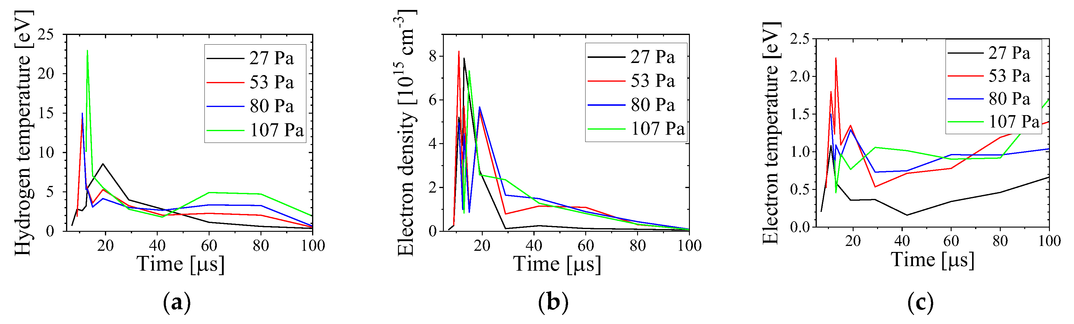
is reached. Results of this analysis for different Hydrogen gas pressure are presented in
Figure 14. The electron density reaches ~8×10
15 cm
-3 within the first ~15 µs followed by a decrease within 70 µs to <10
15 cm
-3. The hydrogen temperature reaches ~25 eV and later decrease to ~3 eV. A relatively large temperature of the hydrogen can be explained by a possible Doppler shift of the spectral lines due to radial motion of the hydrogen atoms, resulting in a thermal temperature which can be significantly smaller. Also, using the calculated plasma electron density, we estimated the electron temperature
using another approximate expression [
25]:
The temperature of electrons was ≤ 2.5 eV which indicates a small degree of ionization of the neutral gas.
Additionally, assuming a Boltzmann distribution of the quantum states population, the plasma electron temperature can be found using the ratio between
and
spectral line integral intensities [
24]:
Here is the integral intensity of the spectral line, is the frequency of the emitted photon for the transition, is the Einstein coefficient for the same transition, and are the degeneracy and energy of the level, respectively, and is the electron temperature. This estimate also results in ≤ 2 eV electron temperatures.
In the case of Helium plasma, the electron temperature was estimated using a Boltzmann plot as [
26]:
Here, is the wavelength of the emitted photon, is the energy difference between the upper and lower energy levels, is the degeneracy of the upper level and C is a constant.
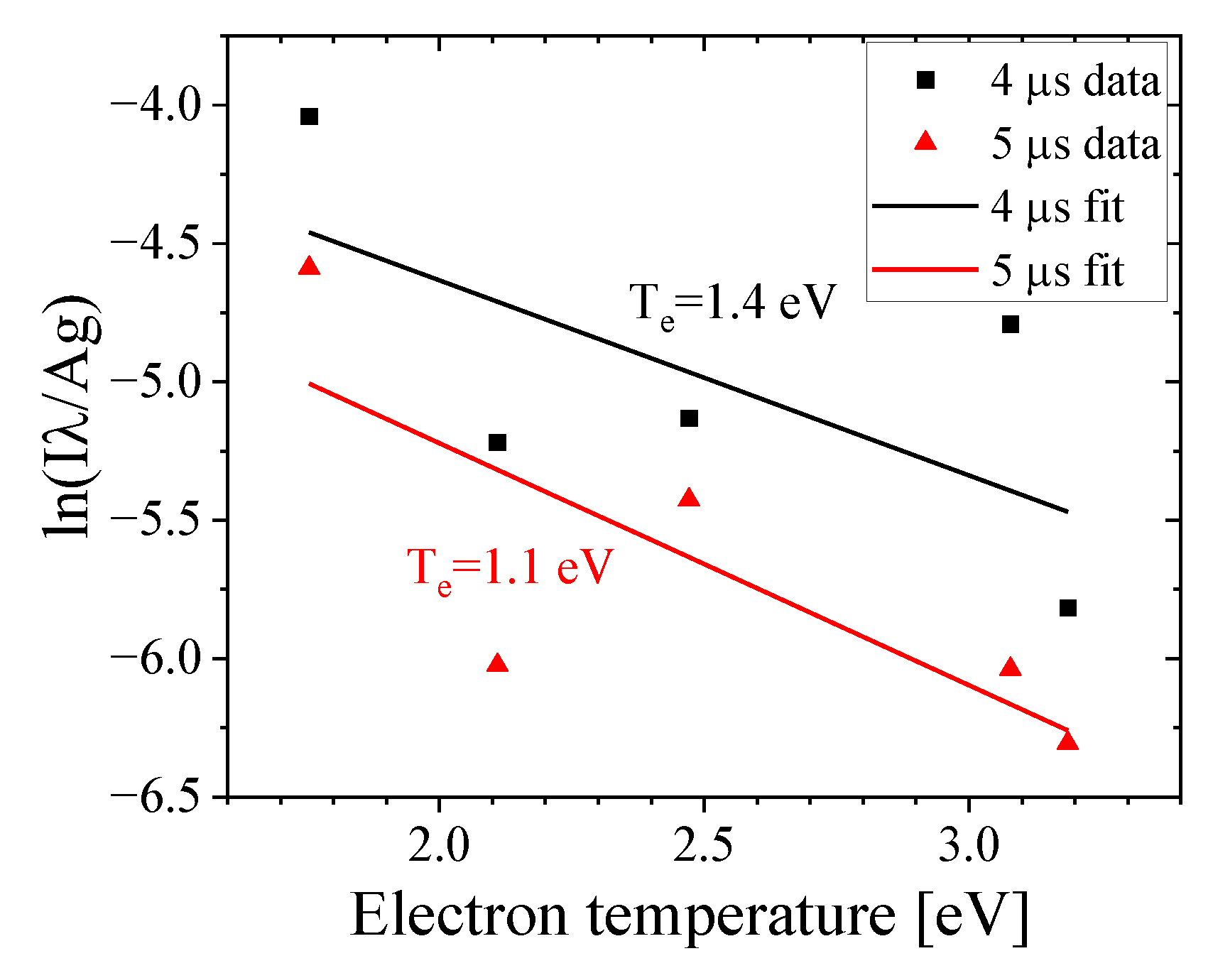
Spectral lines of He I 388, 402, 501, 587 and 706 nm were measured prior to the plasma compression (~4 μs) and during compression (~5 μs). In
Figure 15, a linear fit of the Boltzmann plot is presented, resulting in an electron temperature of < 1.5 eV, similar to the results with Hydrogen plasma.
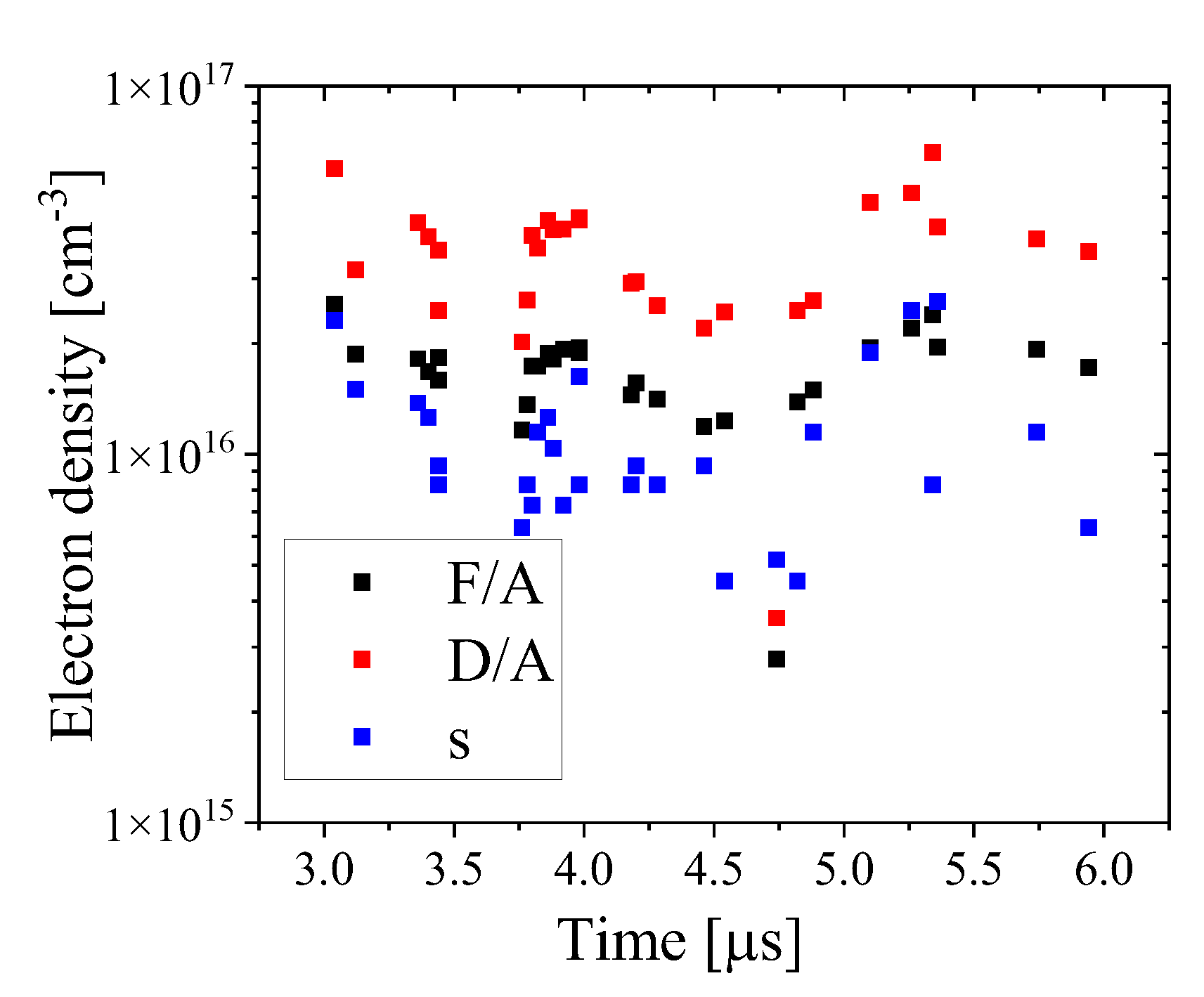
Moreover, for Helium plasma we used the forbidden transition 2
3P - 4
3F of the He I 447.1 nm line to obtain the plasma electron density using relations [
27,
28]:
Here
is the electron density in
, F and A are the amplitudes of the forbidden and allowed lines, respectively, D is amplitude of the dip between the lines, and s is the difference in wavelength between the lines in nm. Comparison between the three relations shows consistent results (
Figure 16).
3.5. Thomson Scattering
During plasma compression, the electron energy distribution function changes in time. The most appropriate method to study the evolution of this distribution function is by Thomson scattering measurements. Calculating the scattering of electromagnetic (EM) radiation in the plasma the electron oscillations due to rapidly changing fields of EM waves need to be considered. These oscillations of the plasma electrons and the resulting electron trajectories are very complex, even when it is assumed that the electrons do not interact with each other. As an EM wave propagates through the plasma, each electron oscillates according to the alternating electrical field of the wave. For a dilute plasma, one can neglect the Coulomb interaction between electrons and ions and therefore the scattered EM waves will only be broadened due to electron temperature (Doppler effect) resulting in a Gaussian broadening of the scattered spectral line FWHM can be used to calculate the electron temperature.
For dense plasmas, the fields produced by neighboring electrons and ions cannot be neglected. Electron and ion density fluctuations contribute small Coulomb perturbations to the electron trajectories. Therefore, the scattered photons are not considered as interacting with each electron, but rather scattered by these electron density fluctuations. These fluctuations lead to various features in the scattering spectrum. In order to distinguish between the different behaviors of the scattered radiation, the Salpeter parameter [
29] is used, defined as
, where
is the wavelength of the laser,
≈
are the wavevectors of the incident and scattered photons
is the angle between the incident and scattered wave vectors and
is the Debye radius of the plasma. For
and
one obtains
, where electron density is in units of 10
16cm
-3 and electron temperature is in eV.
The value of is a fixed parameter determined by the observed angle of the scattered light and the Debye radius , which depends on the electron density and electron and ion temperatures. A large value of corresponds to low density, low temperature plasma. For this case, Coulomb interactions of charged particles are weak giving a Salpeter parameter value of . In this regime electrons are uncorrelated (electrons are moving almost freely in the plasma) and this is the regime of non-collective scattering. This is an analogue to saying that the laser wavelength is much smaller than the Debye length.
However, when
, corresponding to the condition of
, collective effects are to be considered. Laser photons are not considered not to be scattered by free electrons, but by a perturbed electron cloud density of a specific electron plasma frequency and by electrons coupled to ions in the Debye sphere. Thus, the spectrum of the scattered light has two components, labeled as the electron and ion parts. The electron part, having a higher frequency, is shifted to both sides of the central laser wavelength due to collective plasma electron frequency oscillations. Assuming that this process is comparable to an inverse Compton scattering of the laser photon from an ensemble of coupled electrons oscillating with
the plasma electron density can be roughly estimated by measuring the shifted
of the electron part as:
. The ion part appears due to the photons scattered by the electrons coupled to ions in the Debye sphere. Ion thermal motion and ion acoustic waves, manifested as plasma density perturbations, affect the ion coupled electrons which experience these displacements. This results in the broadening of the central ion part, as well as in the appearance of two symmetrical intensity peaks when photon scattering from ion acoustic oscillations is dominant. The frequency separation of these two peaks can be used to estimate the electron temperature. Analyzing the electron density fluctuation yields to an expression of the spectral density function (SDF) [
29]:
Here is the plasma dielectric constant and is the electron (e) and ion (i) electric susceptibility, respectively. Assuming that is the Boltzmann distribution, one can see that when , the spectrum is just a Gaussian function due to Doppler broadening of the scattered photons by free electrons having finite temperature. However, when is not negligible, one obtains a high frequency feature owing to the electron plasma frequency. Additionally, the low frequency ion feature is no longer Gaussian and depends on the plasma ion and electron temperatures and density.
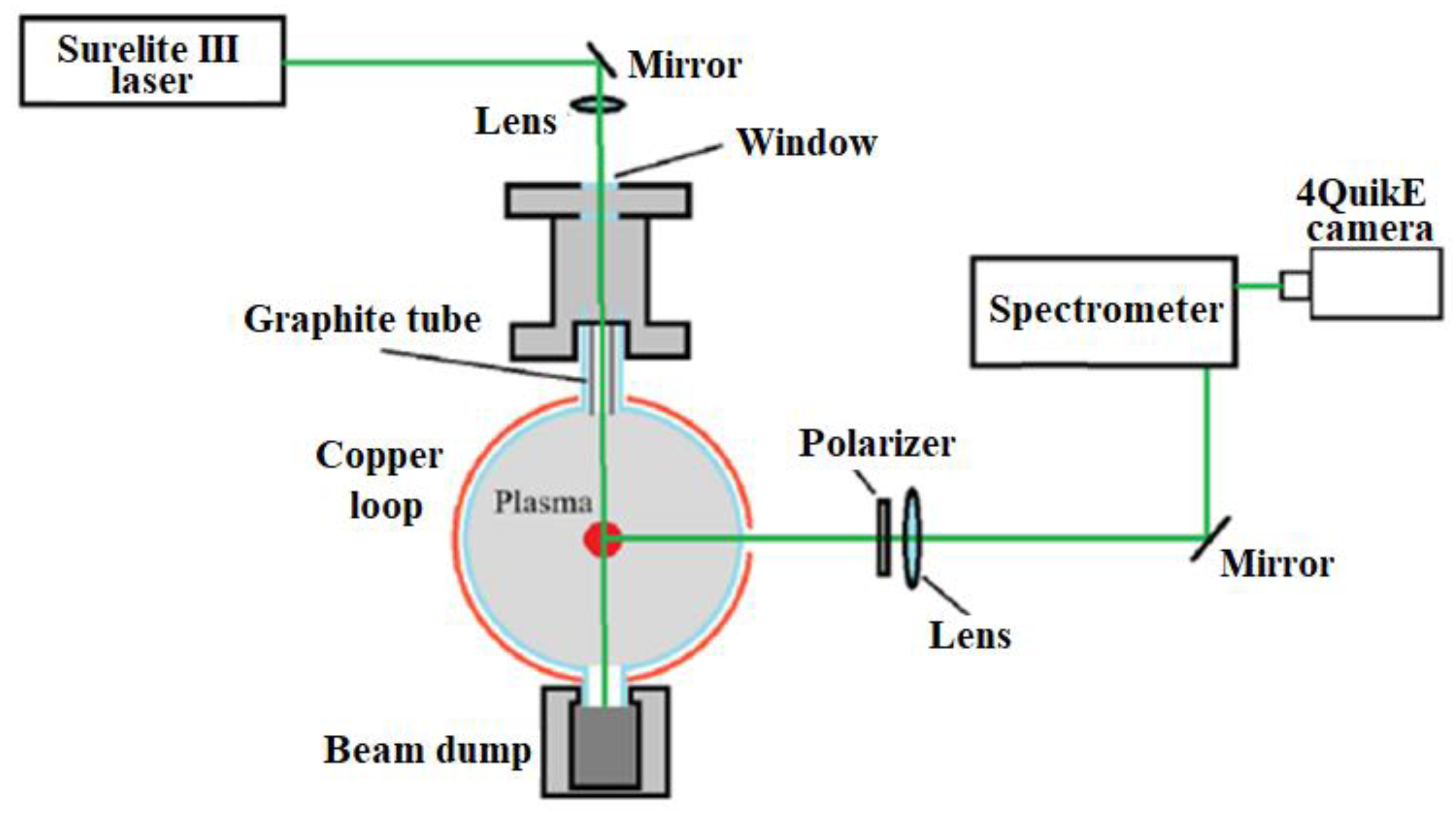
In our experiments, a Surelite III Nd:YAG laser’s second harmonic at 532 nm with 4 ns pulse duration and 350 mJ/pulse energy is focused at the location of the plasma compression region. To minimize parasitic scattered light of the laser beam from the walls of the tube, collimators and a graphite damper were used (see
Figure 17). Scattered light is collected perpendicular to the beam’s path into a spectrometer. In these experiments, for each feature in the SDF different spectrometers were used. With plasma electron density estimated to be
during compression, as found in previous experiments, the Salpeter parameter is calculated as
for electron temperatures < 75 eV. Thus, at compression, the plasma is dense and collective plasma behavior should be considered. The central line profile was observed using the same spectrometer used in the emission spectroscopy experiments, and the electron features were observed using a 25 cm focal length spectrometer with 600 grooves/mm corresponding to a resolution of 1.7 A/pixel.
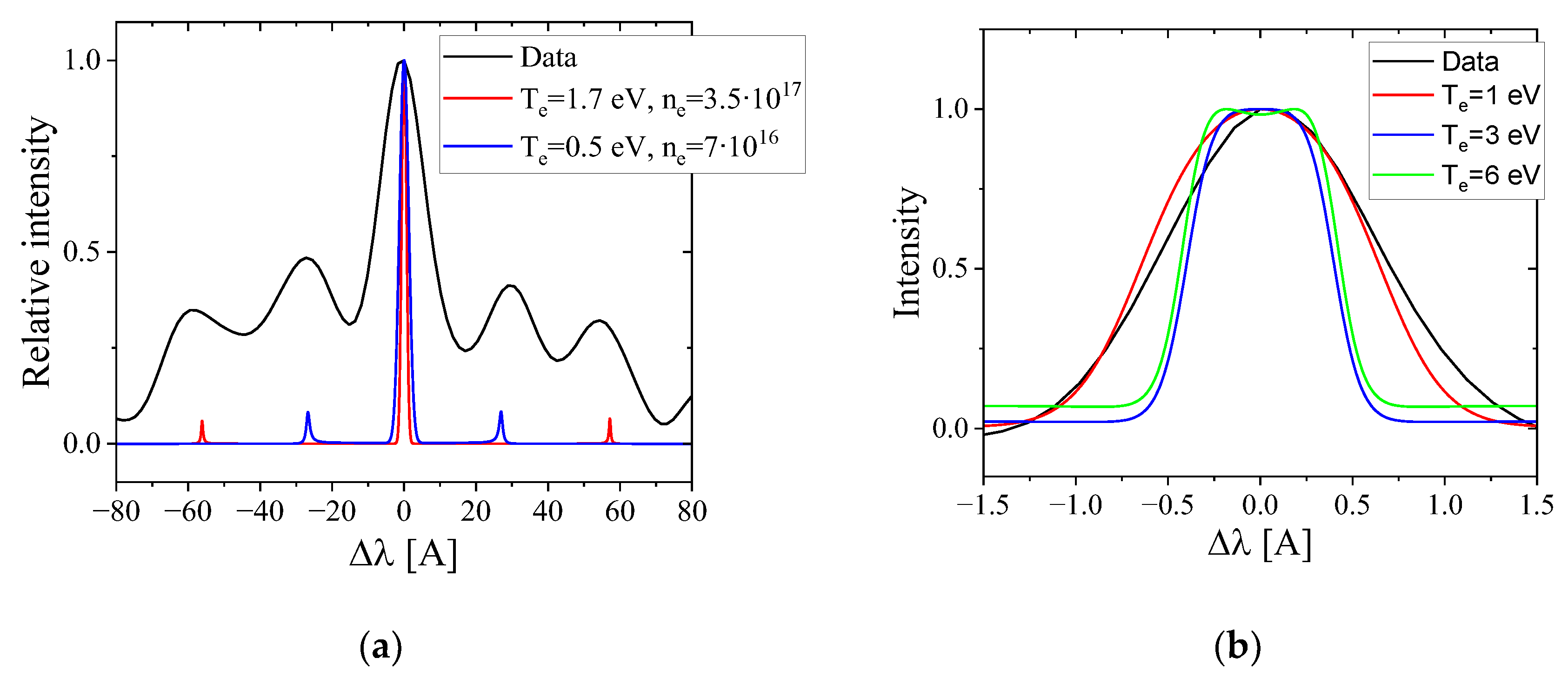
In
Figure 18 (
a) electron features, presented as symmetric peaks, appearing with ~2 nm and 5 nm shifts from the central line are visible. The electron part’s study by numerical calculation of the SDF show that the best fit of these peaks can be obtained for plasma densities ~5×10
16 cm-3 and ~5×10
17 cm-3 with electron temperatures ~1.7 eV and ~0.5 eV, respectively. Central line analysis [see
Figure 18(
b)] confirms the spectroscopic results with ion temperature reaching 20-25 eV during the plasma’s main compression for both Hydrogen and Helium at 53 Pa pressure.
3.6. Laser Induced Fluorescence (LIF)
We applied LIF to study neutral atom temperatures utilizing a 4-energy quantum levels scheme for He plasma. In a Helium atom, a 667.82 nm photon excites an electron transition from the 21P level to the 31D level. Electrons of the 31D level populate the 31P level and spontaneously decay from this level to the 21S level emitting a 501.6 nm photon. Changing the wavelength of the dye laser to ~667.82 nm and measuring the intensity of the 501.6 nm 31P – 21S transition fluorescence photons, He atoms with different velocities along the laser beam direction, were observed.
The experimental setup for LIF measurements is shown in
Figure 19. A ND6000 dye laser was pumped by a Nd:YAG Surelite III laser’s 2nd harmonic, 532 nm, of ~4 ns pulse duration and ~350 mJ/pulse energy. The dyes used are 176 mg/liter DCM dissolved in DMSO (Dimethyl sulfoxide) in the oscillator and 24 mg/liter DCM dissolved in methanol in the amplifiers, resulting in an output pulse of ~4 ns duration with ~4.4 mJ/pulse energy at 667.82 nm. The dye laser beam passes an expander consisting of a 3-mm diameter iris and 2.5 cm and 5 cm focal length lenses to produce a beam of 6-mm diameter. After the expander, the ~2.5 mJ/pulse energy laser beam was directed perpendicularly to the tube axis. The fluorescence photons were collected using a 170-mm focal length lens to a 1-m focus spectrometer with a grating of 2400 grooves/mm. The spectral resolution of the setup was calibrated using Oriel spectral lamps and 4QuikE intensified camera installed at the output of the spectrometer. The calibration factor was 0.123 A/pixel resolution at 501 nm. The spectrometer acts as a spectral filter with a range of
. In experiments with plasma, the intensity of the spectral line at the output of the spectrometer was measured by a Hamamatsu R988U-210 photo multiplier tube (PMT) with 580 V MCP gain.
In a He plasma, measurements at various times of plasma evolution showed that the LIF signal disappears ~ 250 ns prior to the first plasma compression and reappears ≥ 50 μs after this compression. In these experiments, the He gas density in the tube was
. Results of laser interferometry and spectroscopy showed that the plasma electron density is in the range
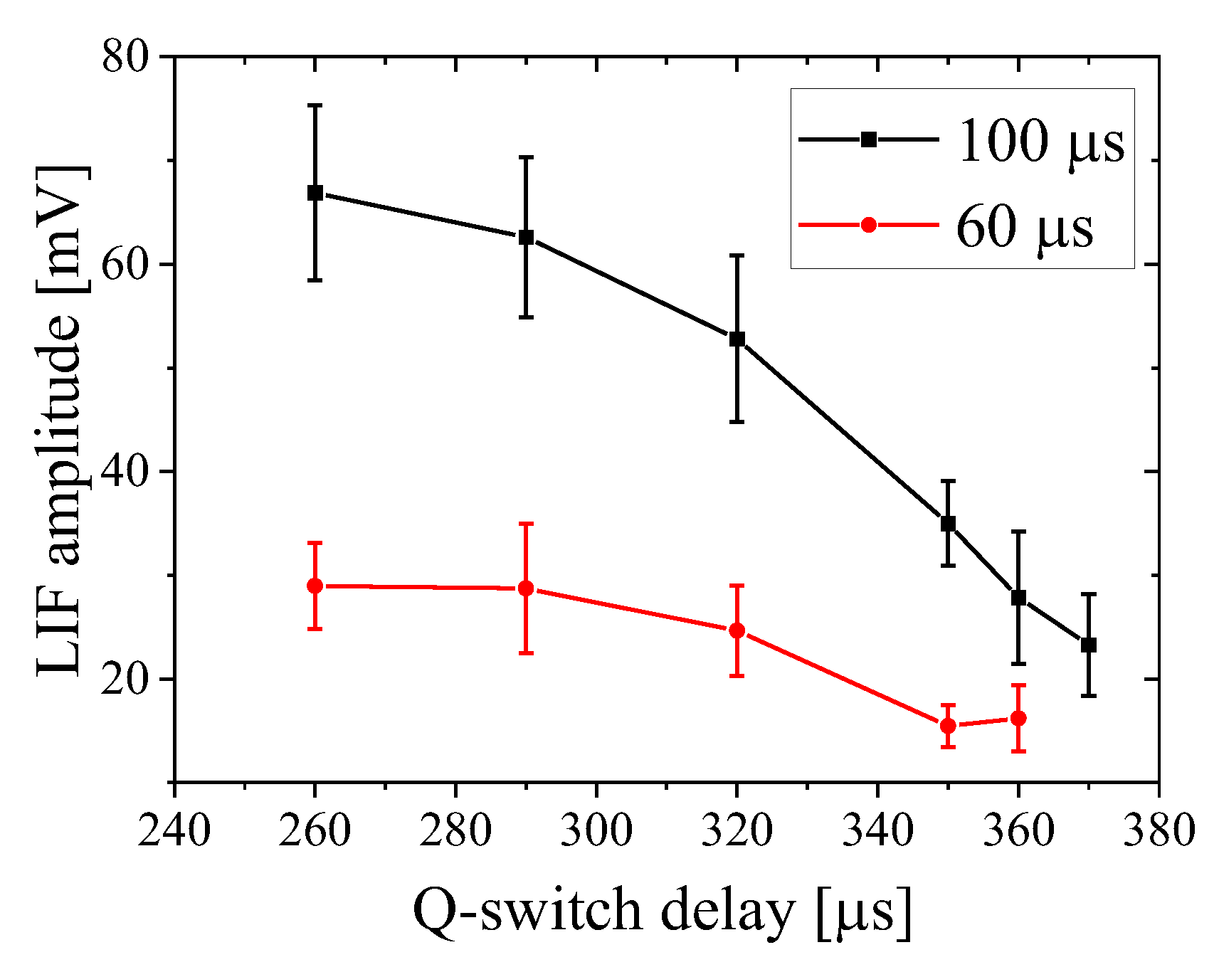
at a time close to the plasma compression. Therefore, it is reasonable to assume that the LIF signal’s disappearance is due to the low density of neutrals in the plasma close to its compression time and it reappears as the neutral density rises with plasma recombination. LIF measurements were carried out at ~300 ns before the plasma first compression and at ~60 μs and ~100 μs after the compression. To avoid saturation of the LIF signal, which results in artificial spectral line broadening, we obtained the dependence of the LIF signal amplitude on the time delay of the Q-switch of the Surelite laser which determines the output energy of the laser beam (see
Figure 20). At ~290 µs time delay the LIF signal saturates. Thus, a 330 μs Q-switch delay was chosen, corresponding to ~1 mJ/pulse energy of the dye laser.
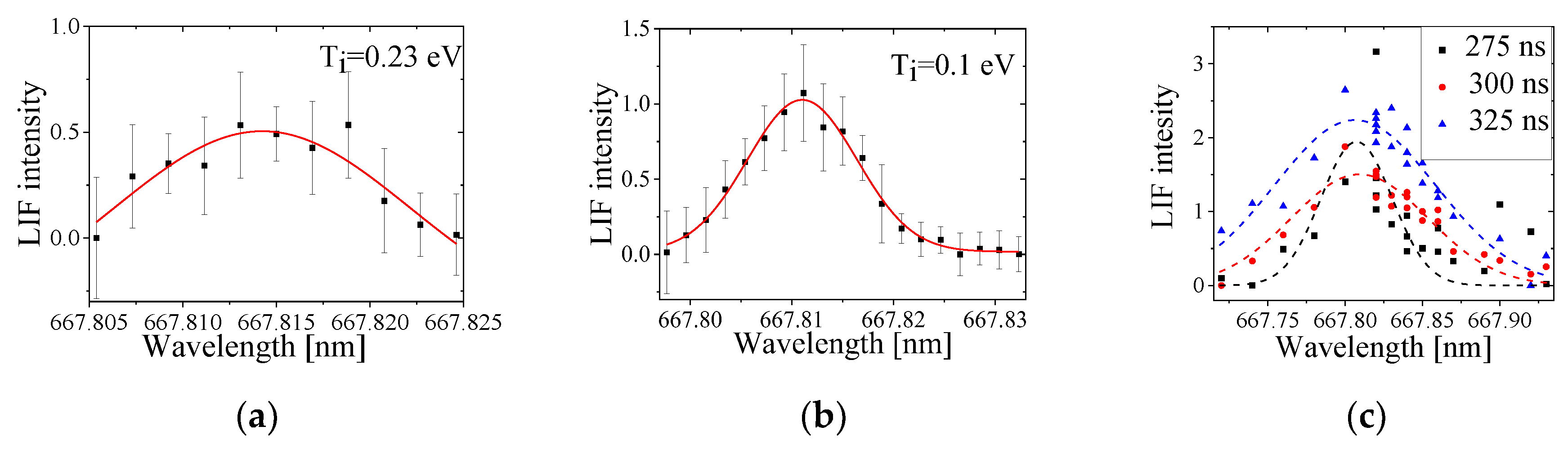
Fluorescence spectral line intensity profiles obtained at 60 μs and 100 μs of the temporal plasma evolution are shown in
Figure 21. At these times, far from compression, the plasma can be considered in thermal equilibrium so that the spectral lines can be analyzed by using only Doppler broadening.
Figure 21(
a) and
Figure 21(
b) demonstrate that the He atoms temperature decreases from 0.26 eV to 0.1 eV at 60 μs and 100 μs, respectively. Close to compression, the plasma dynamics is more complicated since spectral line broadening consists of Doppler shift due to plasma propagation towards the axis and Doppler broadening due to the finite plasma ion temperature. Thus, we can consider only an effective temperature of the He I atoms. Here we assumed that the temperatures of He II and He I are equal due to high collision frequency.
Figure 21(
c) shows that the He I spectral lines obtained 275 ns, 300 ns and 375 ns prior to compression result in effective temperatures 2 eV, 4 eV and 10 eV, respectively.
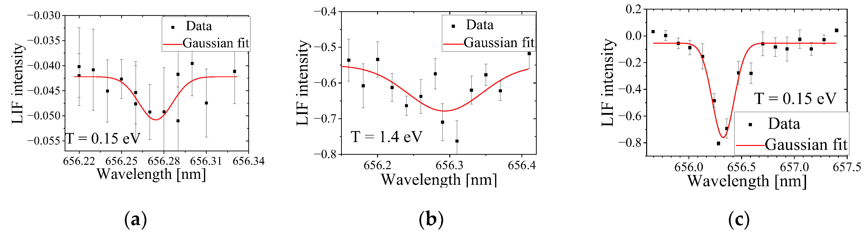
For Hydrogen plasma, LIF was carried out by changing the wavelength of the dye laser close to the
spectral line and measuring the change in intensity of this spectral line. In these experiments, we first measured the
intensity without the dye laser, the background intensity. Then, with the dye laser, this background intensity was subtracted from the PMT signal, resulting in the LIF profile of the
spectral line (see
Figure 22). These measurements, carried out at various times of the plasma evolution, show that Hydrogen atoms temperature does not exceed < 2 eV at the time of the plasma compression.
4. Summary
In this article we presented results characterizing a small and compact Theta Pinch using different non-perturbing, time and space resolved diagnostics. In addition to electrical measurements of the discharge current, the results of various diagnostic methods and their analysis were presented. The methods we used were: microwave cut-off, laser interferometry, visible spectroscopy, Thomson scattering and LIF. Using these methods the plasma density and temperature evolution were obtained and the results from different diagnostic methods found to be in a satisfactory agreement. Thus, using these diagnostics the parameters of the plasma in the device developing in Nt-TAO can be studied with high reliability.
Author Contributions
Methodology, Yakov Krasik; Software, Sagi Turiel and Daniel Maler; Validation, Sagi Turiel and Alexander Gribov; Investigation, Sagi Turiel, Alexander Gribov and Daniel Maler; Resources, Alexander Gribov; Writing – original draft, Sagi Turiel and Daniel Maler; Writing – review & editing, Yakov Krasik; Supervision, Yakov Krasik.
Funding
This research was funded by Israeli National Authority for Technological Innovation “Magneton”, grant number 880326.
Data Availability Statement
The original contributions presented in this study are included in the article. Further inquiries can be directed to the corresponding author(s).
Acknowledgments
We are grateful to J. G. Leopold, I. Gissis for fruitful discussions and E. Flyat for generous technical assistance. This research was supported by the Israeli National Authority for Technological Innovation “Magneton” (Grant number 880326).
Conflicts of Interest
The authors declare no conflicts of interest.
References
- Green, T.S. Evidence for the containment of a hot, dense plasma in a theta pinch. Phys. Rev. Lett. 1960, 5, 297–300. [Google Scholar] [CrossRef]
- Jahoda, F.C.; Little, E.M.; Quinn, W.E.; Ribe, F.L.; Sawyer, G.A. Plasma Experiments with a 570-kJ Theta-Pinch. J. Appl. Phys. 1964, 35, 2351–2363. [Google Scholar] [CrossRef]
- Taylor, J.B.; Wesson, J.A. End losses from a theta pinch. Nucl. Fusion. 1964, 5, 159. [Google Scholar] [CrossRef]
- Little, E.M.; Quinn, W.E.; Sawyer, G.A. Plasma End Losses and Heating in the ``Low-Pressure'', Regime of a Theta Pinch. Phys. Fluids. 1965, 8, 1168–1175. [Google Scholar] [CrossRef]
- Silberg, P.Q. Some Efficiency Measurements of the Theta-Pinch. J. Appl. Phys. 1966, 37, 2155–2161. [Google Scholar] [CrossRef]
- Gribble, R.F.; Little, E.M.; Morse, R.L.; Quinn, W.E. Faraday Rotation Measurements on the Scylla IV Theta Pinch. Phys. Fluids. 1968, 11, 1221–1226. [Google Scholar] [CrossRef]
- Yarborough, W.W.; Barach, J.P. Current sheet observations in a small theta pinch. Phys. Fluids. 1975, 18, 105–108. [Google Scholar] [CrossRef]
- Lee, S. Radiations in Plasmas; McNamara, B., Ed.; World Scientific: Singapore, 1984; pp. 978–987. [Google Scholar]
- McKenna, K.F.; Siemon, R.E. Theta-pinch research at Los Alamos. Nucl. Fusion. 1985, 25, 1267. [Google Scholar] [CrossRef]
- Luna, F.R.T.; Cavalcantiz, G.H.; Trigueirosy, A.G. A theta-pinch as a spectroscopic light source. J. Phys. D: Appl. Phys. 1998, 31, 866–872. [Google Scholar] [CrossRef]
- Awe, T.J.; Siemon, R.E.; Bauer, B.S.; Fuelling, S.; Makhin, V.; Hsu, S.C.; Intrator, T.P. Magnetic Field and Inductance Calculations in Theta-Pinch and Z-Pinch Geometries. J. Fusion Energy. 2006, 26, 17–20. [Google Scholar] [CrossRef]
- Lee, S.; Lee, P.; Saw, S.H.; Rawat, R.S. Numerical experiments on plasma focus pinch current limitation. Plasma Phys. Control. Fusion. 2008, 50, 065012. [Google Scholar] [CrossRef]
- Cavalcanti, G.H.; Farias, E.E. Analysis of the energetic parameters of a theta pinch. Rev. Sci. Instrum. 2009, 80, 125109. [Google Scholar] [CrossRef] [PubMed]
- Jung, S.; Surla, V.; Gray, T.K.; Andruczyk, D.; Ruzic, D.N. Characterization of a theta-pinch plasma using triple probe diagnostic. J. J. Nuclear Materials. 2011, 415, 993–995. [Google Scholar] [CrossRef]
- Chaisombata, S.; Ngamrungroj, D.; Tangjitsomboona, P.; Mongkolnavina, R. Determination of Plasma Electron Temperature in a Pulsed Inductively Coupled Plasma (PICP) device. In Proceedings of Engineering. 2012, 32, 929–935. [Google Scholar] [CrossRef]
- Lee, S.; Saw, S.H.; Lee, P.C.K.; Akel, M.; Damideh, V.; Khattak, N.A.D.; Mongkolnavin, R.; Paosawatyanyong, B. A model code for the radiative theta pinch. Phys. Plasmas. 2014, 21, 072501. [Google Scholar] [CrossRef]
- Ebrahim, F.A.; Gaber, W.H.; Abdel-Kader, M.E. Estimation of the Current Sheath Dynamics and Magnetic Field for Theta Pinch by Snow Plow Model Simulation. J. Fusion Energy. 2019, 38, 539–547. [Google Scholar] [CrossRef]
- Cistakov, K.; Christ, P.; Manganelli, L.; Gavrilin, R.; Khurchiev, A.; Savin, S.; Iberler, M. Study on a dense Theta pinch plasma for ion beam stripping application for FAIR. J. Recent Contrib. Phys. 2020, 4, 14–20. [Google Scholar] [CrossRef]
- Christ, P.; Cistakov, K.; Iberler, M.; Laghchioua LMann, D.; Rosmej, O.; Savin SJacoby, J. Measurement of the free electron line density in a spherical theta-pinch plasma target by single wavelength interferometry. J. Phys. D Appl. Phys. 2021, 54, 285203. [Google Scholar] [CrossRef]
- Wang, Z.; Cheng, R.; Wang, G.; Jin, X.; Tang, Y.; Chen, Y.; Zhou, Z.; Shi, L.; Wang, Y.; Lei Yu Wu, X.; Yang, J. Observation of plasma dynamics in a theta pinch by a novel method. Matter Radiat. Extremes. 2023, 8, 045901. [Google Scholar] [CrossRef]
- Djorovic, S.; Pavlov, M. Measurements of specific heats ratio of hydrogen plasmas. Beitr. Plasmaphys. 1984, 24, 105–112. [Google Scholar] [CrossRef]
- https://www.nt-tao.com/.
- Raizer, Y.P. Gas Discharge Physics; Publisher: Springer, 1997. [Google Scholar]
- Griem, H.R. Principles of Plasma Spectroscopy; Publisher: Cambridge University Press, 1997. [Google Scholar]
- Konjević, N.; Ivković, M.; Sakan, N. Spectrochim. Acta - Part B At. Spectrosc 2012, 76, 16. [CrossRef]
- Ohno, N.; Razzak, M.A.; Ukai, H.; Takamura Sh Uesugi, Y. Validity of Electron Temperature Measurement by Using Boltzmann Plot Method in Radio Frequency Inductive Discharge in the Atmospheric Pressure Range. Plasma and Fusion Research. 2006, 1, 28. [Google Scholar] [CrossRef]
- Perez, C.; Santamarta, R.; de la Rosa, M.I.; Mar, S. Stark broadening of neutral helium lines and spectroscopic diagnostics. Eur. Phys. J. 2003, 27, 73–75. [Google Scholar]
- Czernichowski, A.; Chapelle, J. Use of 447 nm He I line to determine electron concentration. J. Quant. Spectrosc. Radiat. Transfer. 1985, 33, 427–435. [Google Scholar] [CrossRef]
- Sheffield, J.; Froula, D.; Glenzer, S.H., Luhmann, N.C., Jr. Plasma Scattering of Electromagnetic Radiation, Second Edition: Theory and Measurement Techniques. Hardback ISBN: 9780123748775, eBook ISBN: 9780080952031, 2010.
Figure 1.
The experimental setup used to produce a Theta Pinch with a single loop.
Figure 1.
The experimental setup used to produce a Theta Pinch with a single loop.
Figure 2.
Waveforms of the current for the 1 μF capacitor charged to 17 kV and discharged into the 3-loop coil (black line) and two 0.44 μF capacitors connected in parallel, charged to 25 kV and discharged into a single loop coil (red dashed line). The He gas pressure in the tube was 0.1 Pa.
Figure 2.
Waveforms of the current for the 1 μF capacitor charged to 17 kV and discharged into the 3-loop coil (black line) and two 0.44 μF capacitors connected in parallel, charged to 25 kV and discharged into a single loop coil (red dashed line). The He gas pressure in the tube was 0.1 Pa.
Figure 3.
Three-loops coil Theta Pinch; (a) Waveforms of the discharge current at 2.7 kPa pressure when no plasma generation was obtained (black) and with the plasma generation at 0.4 kPa (red) pressure of He gas; (b) Energy deposited into the gas discharge vs. gas pressure for He (black squares) and H2 (red dots).
Figure 4.
Single loop Theta Pinch; (a) Waveforms of the discharge current obtained in the case of Helium gas at 0.1 Pa pressure when no plasma generation was obtained (black) and with plasma generation at 0.4 kPa (red) pressure of He gas; (b) Energy deposited into the gas discharge versus He (black squares) and H2 (red dots) pressure.
Figure 5.
Front view frame images of the light emission (top row) obtained at different times of plasma compression for a single loop Theta Pinch at Hydrogen pressure of 63 Pa and at frame duration of 10 ns and side view frame images of light emission (bottom row) obtained at different times for the 3-loops setup at Hydrogen pressure of 106 Pa and at frame duration of 10 ns.
Figure 6.
Typical waveforms of current (black) and photodiode light intensity (red) obtained for single loop (a) and for 3-loop (b) setups for 63 Pa Hydrogen.
Figure 6.
Typical waveforms of current (black) and photodiode light intensity (red) obtained for single loop (a) and for 3-loop (b) setups for 63 Pa Hydrogen.
Figure 7.
Lee model current (solid black) compared with the measured current (dashed black) for a single loop (a) and for the 3-loop (b) setups and calculated shock (red) and piston (blue) radii during initial compression. He gas pressure is of 63 Pa.
Figure 7.
Lee model current (solid black) compared with the measured current (dashed black) for a single loop (a) and for the 3-loop (b) setups and calculated shock (red) and piston (blue) radii during initial compression. He gas pressure is of 63 Pa.
Figure 8.
Microwave cutoff setup for a 3-loop Theta Pinch setup. (1) 32 V DC source, (2) the klystron and antenna (70 GHz), (3) receiving antenna with the Schottky diode, (4) photodiode, (5) Pierson current monitor. Microwaves are marked as green arrows.
Figure 8.
Microwave cutoff setup for a 3-loop Theta Pinch setup. (1) 32 V DC source, (2) the klystron and antenna (70 GHz), (3) receiving antenna with the Schottky diode, (4) photodiode, (5) Pierson current monitor. Microwaves are marked as green arrows.
Figure 9.
Typical waveforms of the discharge current, light emission and transmitted microwave intensity (a) obtained for Helium at 63 Pa pressure. The transmitted microwave intensity for Hydrogen (b) and Helium (c) plasma experiments at different gas pressures. All results are for the 3-loop setup.
Figure 10.
Michelson interferometer set up for average plasma density measurements for a 3-loop Theta Pinch experiment. (1) Laser; (2) beam splitter; (3) and (4) mirrors; (5) bandpass filter matching the laser wavelength; (6) photodiode; (7) ND filter.
Figure 10.
Michelson interferometer set up for average plasma density measurements for a 3-loop Theta Pinch experiment. (1) Laser; (2) beam splitter; (3) and (4) mirrors; (5) bandpass filter matching the laser wavelength; (6) photodiode; (7) ND filter.
Figure 11.
(A) Interference waveform measured on a ms-timescale ; (b) Interference waveform measured on a 100 μs time scale; (c) Electron density (black) and discharge current in relative units (red) for 53 Pa Hydrogen plasma and a 3-loop setup.
Figure 11.
(A) Interference waveform measured on a ms-timescale ; (b) Interference waveform measured on a 100 μs time scale; (c) Electron density (black) and discharge current in relative units (red) for 53 Pa Hydrogen plasma and a 3-loop setup.
Figure 12.
Electron density evolution at different pressures of a Hydrogen plasma using the green laser (a) and the red laser (b) and (c) a Helium plasma (green laser) for a 3-loop Theta Pinch setup.
Figure 12.
Electron density evolution at different pressures of a Hydrogen plasma using the green laser (a) and the red laser (b) and (c) a Helium plasma (green laser) for a 3-loop Theta Pinch setup.
Figure 13.
Spectroscopy setup. A single loop setup.
Figure 13.
Spectroscopy setup. A single loop setup.
Figure 14.
(A) Ion temperature; (b)electron density; and (c) electron temperature calculated for Hydrogen plasma at various gas pressures for the 3-loops setup.
Figure 14.
(A) Ion temperature; (b)electron density; and (c) electron temperature calculated for Hydrogen plasma at various gas pressures for the 3-loops setup.
Figure 15.
Electron temperatures estimated 4 and 5 μs after the start of the current, using a Boltzmann plot.
Figure 15.
Electron temperatures estimated 4 and 5 μs after the start of the current, using a Boltzmann plot.
Figure 16.
Electron density calculated using the three relations involving the Forbidden - Allowed transition of the 447.1 spectral line of He I atom.
Figure 16.
Electron density calculated using the three relations involving the Forbidden - Allowed transition of the 447.1 spectral line of He I atom.
Figure 17.
Setup for Thomson scattering experiment. Single loop setup.
Figure 17.
Setup for Thomson scattering experiment. Single loop setup.
Figure 18.
(A)Thomson scattering spectrum measured for 53 Pa Hydrogen gas pressure at the time of plasma compression with ~20 eV ion temperature (black) compared to the numerical SDF with the same ion temperature for different electron temperature and density; (b) The central spectral feature measured with the high resolution spectrometer at the same time and same gas pressure (black) compared with the SDF calculated for for different .
Figure 19.
Experimental setup for Helium LIF measurements. Single loop setup.
Figure 19.
Experimental setup for Helium LIF measurements. Single loop setup.
Figure 20.
Dependence of the LIF amplitude measured at 100 μs and 60 μs after the plasma compression vs. the Q-switch delay time.
Figure 20.
Dependence of the LIF amplitude measured at 100 μs and 60 μs after the plasma compression vs. the Q-switch delay time.
Figure 21.
LIF spectral line profiles measured at 60 μs (a) and 100 μs (b) after the plasma compression and at ~275 ns, ~300 ns and ~375 ns before the plasma compression (c).
Figure 21.
LIF spectral line profiles measured at 60 μs (a) and 100 μs (b) after the plasma compression and at ~275 ns, ~300 ns and ~375 ns before the plasma compression (c).
Figure 22.
LIF intensity of vs. the wavelength of the dye laser at different time delays relative to the first plasma compression. (a) 300 ns prior to plasma compression, (b) At the time of the plasma compression and (c) after the plasma.
Figure 22.
LIF intensity of vs. the wavelength of the dye laser at different time delays relative to the first plasma compression. (a) 300 ns prior to plasma compression, (b) At the time of the plasma compression and (c) after the plasma.
|
Disclaimer/Publisher’s Note: The statements, opinions and data contained in all publications are solely those of the individual author(s) and contributor(s) and not of MDPI and/or the editor(s). MDPI and/or the editor(s) disclaim responsibility for any injury to people or property resulting from any ideas, methods, instructions or products referred to in the content. |
© 2024 by the authors. Licensee MDPI, Basel, Switzerland. This article is an open access article distributed under the terms and conditions of the Creative Commons Attribution (CC BY) license (http://creativecommons.org/licenses/by/4.0/).