
Submitted:
14 November 2024
Posted:
14 November 2024
You are already at the latest version
Abstract
To study the process of concrete degradation, the so-called spatiotemporal waveform profiles were obtained, which are sets of ultrasonic signals acquired by step-by-step surface profiling of the concrete surface. The recorded signals were analyzed and informative areas for three fre-quencies were identified. The type of the created neural network is a multilayer perceptron. Stochastic gradient descent was chosen as the learning algorithm. Measurement datasets (test, training and validation) were created to determine two factors of interest - the degree of materi-al degradation and the thickness (depth) of the degraded layer. The article proves that the train-ing datasets are quite sufficient to obtain acceptable results. It is shown that the results for the Fourier amplitude spectra are significantly worse than the results of neural networks built on the basis of information about the measured signals themselves.
Keywords:
ultrasonic testing
; neural networks
; concrete
; surface degradation
1. Introduction
Concrete is the most used building material in the world initially designed for long-term operation of at least 50 years, and for infrastructure objects at least 100 years. Concrete infrastructure, buildings and industrial objects made of concrete are aging and deteriorating causing the need for remedial measures to reinstate their safety and serviceability [1]. In case of premature degradation of concrete, there is a need for its timely repair, restoration and, in the worst case, replacement of structures. This significantly worsens the environmental and cost components of the concrete life cycle. Cement production accounts for 5-8% of global CO2 emissions [2]. Moreover, accordingly, one cubic meter of produced concrete is responsible for 200 to 400 kg of emitted CO2. Therefore, timely diagnostics of concrete structures is an important component of ensuring their safety and a factor in sustainable development.
The effects of environmental factors, such as moisture, freeze-thaw cycles, water ingress, chemical attack and carbonation and internal factors, such as forces, alkali-aggregate reactions are the main sources of the material degradation and cracking [3]. Progressive deterioration of concrete occurs at the surface of many structures susceptible to environmental factors. There are several types of concrete degradation in which destruction begins from the surface layer and gradually extend to depth from the concrete surface. Progressing into depth, deterioration of the surface leads to exposure of coarse aggregate and ultimately reinforcing steel. Examples of concrete surface deterioration presented in Figure 1 illustrate the hazard for infrastructural objects in regions, where multiple alternations of frost and warm during a year are combined with a high humidity of the air. Another case of such exposures are concrete hydraulic structures like dams, bridges, spillways, sluices, and weirs, where the damage in fresh waters is similar in appearance to salt scaling of concrete due to leaching of the concrete surface [4]. Also, the carbonization effect begins from the surface layer and over time penetrates into the depth of the material. Usually carbonation is visually imperceptible, it is associated with minor changes in the microstructure of concrete, but when it reaches the steel reinforcement it can contribute to its corrosion. For practical determination of carbonation depth non-destructive methods are necessary. Some researchers propose either theoretical models or destructive methods by taking material samples [5]. The problem of frost resistance is associated with the alternating freezing and thawing of the surface layer of concrete in a saturated state. Most studies show that during cyclic freezing of concrete saturation with salt solutions, gradient stress occurs near the surface, resulting in the phenomenon of delamination and scaling [6].
The phenomenon of explosive spalling and delamination of surface layers is also observed under extreme exposure to high temperatures in case of fire. Diagnostics of the degree of surface destruction is also necessary when assessing the technical condition of high temperature facilities made of refractory concretes [7]. Special impregnating coating is proposed [8] to protect refractory concrete surface from the aggressive effects of combustion products at high temperatures. For this case, a non-destructive method is necessary to determine the penetration depth of the impregnating material.
To evaluate the degree of concrete deterioration as a volumetric process initiated at the surface and progressing into the depth, the adequate assessment of the properties of the surface layer in terms of depth is important. A range of non-destructive testing methods is exploited in the civil and structural engineering industry, infrastructure monitoring services and materials research for assessing the quality of concrete [9,10]. These include surface hardness testers using the Schmidt rebound hammer, penetration resistance methods, radiographic testing, resonant frequency methods and ultrasonic testing. Ultrasonic testing is the most widely used non-destructive technique to evaluate the mechanical condition of concrete in situ by measuring the ultrasound pulse velocity in through or surface transmission in the area of concrete between the emitting and receiving transducers [11,12,13]. The basis for predicting the mechanical status of concrete is empirically obtained correlations between the ultrasound pulse velocity, dynamic modulus of elasticity and compressive strength of concrete [14]. This method is most effective when comparing highly differing conditions in relatively homogeneous concrete structures, for example, during the hardening of concrete or the evaluation of used cement grades. However, being limited to simple solutions for complex problems such as cracks in deep concrete structures, approaches with embedded sensors and advanced processing have been proposed, in particular window-based cross-correlation and continuous wavelet transform extracting information about features of interest (cracks, damages) from raw ultrasonic signals [15]. Ultrasonic surface waves at different frequencies have been proposed to assess the condition of the surface layer of concrete by depth knowing the dependence of the penetration depth of Rayleigh waves on its wavelength [16]. Potential effectiveness of ultrasonic surface waves to assess the thickness of damaged concrete to be removed in bridge structures was demonstrated [17]. The method of surface acoustic waves’ spectroscopy for the assessment of the layered concrete used the dispersion of the phase velocity of surface waves [18].
However, traditional approaches based on the measurement of single parameters such as ultrasound pulse velocity in ultrasonic testing do not allow separating the complex influences of acting factors contributing the quality of the surface layer. For comprehensive characterization of the surface layer of concrete, knowledge of both the strength of the material affected by the degree of its degradation and the depth of the degraded layer is necessary. This prompts the development of new diagnostic approaches and the use of more sophisticated data processing, in particular, using artificial intelligence methods. The method of using so called spatiotemporal waveform profiles or sets of ultrasonic signals collected stepwise along a distance on the concrete surface and further application of the pattern recognition method was proposed to estimate the depth of material degradation [19]. Although the method demonstrated viability, the statistical evaluation criteria applied did not provide the required accuracy in all test cases. Therefore, it was decided to apply neural network analysis in the present study as an alternative data processing.
Solutions to automatize the diagnostic process or at least to provide assistance are currently under active research as a consequence of the digitization of manufacturing processes [20,21]. A deep learning architecture [22] consists of a chain of mathematical operations established between inputs and outputs, the so-called layers. That is, the layers perform transformation on inputs in order to extract the most meaningful features to perform the final tasks (e.g., regression, classification, etc.). In the most common deep learning architecture, the output of one layer is fed to the next layer neuron through a linear combination of weights and biases. These linear operations are subject to an element-by-element nonlinear transformation through the use so-called activation functions (or layers) aimed at handling nonlinear behavior in mapping two successive layers. The most common activation functions are the sigmoid, rectified linear unit (ReLU), etc. The use of a specific activation function depends on the task associated to the layer to which it is attached. From a general point of view, the connections between two layers identifies the architecture type, e.g., fully connected neural network, multi-layer perceptron, convolutional neural network, long short time memory, recurrent neural network, to name just the most prominent ones [23,24,25,26].
For the effective use of neural networks, it is important to use only data sensitive to defects or changes in the properties of the studied structures for their training. For this purpose, many works resort to preliminary analysis of the data obtained: principal component analysis [27], factor analysis [28], statistical techniques [29], Fourier transform [30], wavelet transform [31] or empirical mode decomposition (EMD) [32].
The application of artificial neural networks (ANN) in problems of reconstruction of damaged state of structural elements is described in numerous publications [33,34,35,36,37,38,39,40,41,42], including the use of various architectures and ANN algorithms [43,44,45]. Parameters of a defect were investigated based on the reaction of the layered structure to the sudden pulses [42]. The reconstruction of the defect radius was based on a combination of the calculation of the unsteady oscillations of the plate and the use of ANN. A finite element model of the layered elastic structure was created taking into account the energy dissipation with the help of ANSYS package and calculations were performed for various radius values of the defect. Neural networks were built using MATLAB. The article proved that the volume of data used is sufficient to successfully train the created ANN model and to identify a hidden defect in the structure.
The idea of using pattern recognition and machine learning methods in the problems of assessing the state of concrete building structures has been actively developed during recent years [43]. Analysis of concrete defects using the genetic algorithm - back propagation GA-BP neural network applied to ultrasonic signals processed by wavelet transform was aimed to detect macroscopic defects (holes with a diameter of 5 mm or larger) [44]. Automatic detection of concrete damage used a convolutional neural network was applied to images of concrete objects to identify macroscopic defects on its surface, such as cracks [45]. A method for crack detection and measurement was presented [46], which uses deep learning and image processing to classify, segment, and measure cracks. It allows measuring cracks not in pixels, but in more practical units of measurement - millimeters. A method for assessing a parameter of interest related to material properties using the digital Fourier transform (DFT) and multilayer perceptron (MLP) was intended for identification of carburization level in industrial high-pressure pipes [47].
Along with the presentation of the application of ANN, this work has a broader purpose – to demonstrate the possibilities of diagnosing the state of a complex material with a gradient of changes in properties by depth using the proposed ultrasonic method.
2. Methods and Materials
2.1. Concrete Specimens Modeling Degradation of Surface Layer
The specimens’ design corresponded to the purpose of the study – to explore the possibility of predicting two factors of interest describing the process of deterioration of the concrete surface layer – the degree of the material degradation (D) and the depth or thickness of the degraded layer (ThD). Both of these factors were modeled in this simulation study. Two-layered concrete specimens with gradually varied D and ThD were intended for ultrasonic surface scanning at three ultrasonic frequencies (Figure 2). Conventionally “weak” and “strong” concretes simulated the upper degraded layer and the intact base layers, correspondingly, where the state of the concrete material was determined by changing the cement-to-sand ratio. The set of specimens created a two-dimensional data grid for constructing a mathematical model to recognize the two factors of interest, D and ThD.
Three stages of the conditionally “weak” surface layer D1, D2 and D3 were selected, where the cement-to-sand ratios were: 1:4 for D1; 1:7 for D2; and 1:12 for D3. The cement-to-sand ratio in the “strong” base layer S was 1:3. Based on the measured values of the ultrasonic pulse velocity, which varied from 4400 m/s in the S layer to 2150 m/s in the D3 layer, and the known empirical dependence of the velocity on the compressive strength [4,5], the strength of the layers was approximately predicted as: 36 MPa for S; 25 MPa for D1; 14 MPa for D2; and 8 MPa for D3. The specimens were two-layer rectangular prisms 160x40x40 mm with the degraded surface layer D and the base solid layer S. The thickness of the D layer ThD had 9 gradations: 0, 3, 5, 12, 20, 25, 30, 35 and 40 mm, where the specimens with ThD=0 and ThD=40 mm completely consisted of solid layer S and degraded layer D, respectively. Thus, the total number of specimens in the experiment was 27 (9 ThD grades and 3 D grades).
2.2. Ultrasonic Data Acquisition
To ensure rapid automated data collection and ultrasonic signal acquisition through step-by-step surface profiling, a special scanning setup was developed, which included both mechatronic scanning device and an electronic unit for ultrasonic data collection, synchronized in operation.
The main purpose of the scanning device (Figure 3) was the computer-aided positioning of piezoelectric transducers on a concrete specimen, which could have an inclined and uneven surface. The scanner had one horizontal axis for linear scanning and two parallel vertical axes for lifting and placing the transducers, each driven by stepper motors. The specimen was positioned under a fixed emitting transducer, and the motor drive moved the receiving transducer in a straight line on the specimen’s surface, changing the distance or acoustic base between the transducers in the range from 0 to 150 mm with an accuracy of 0.1 mm. Motor-driven vertical displacement of both the emitting and receiving transducers allowed them to be vertically positioned and pressed against the specimen’s surface with a dosed contact force set by preloading the spring. The scanner was designed as a frame made of aluminum profiles with all components mounted inside it. The mechatronic system consisted of a linear rod and rail movement system with a belt drive and NEMA series hybrid stepper motors. The custom parts were manufactured using an FDM 3D printer. Repeatable positioning was provided by optical limit switches on each vertical axis, which define the “home” position of the device. In addition, optical contact switches on the vertical axes indicated the contact of the transducers with the specimen’s surface. Motion control was performed by a single-board GRBL controller, which is a CNC machine controller receiving G-code commands from a PC via USB. The pre-scan option was intended to obtain data on the specimen’s relief and take it into account during the main test. With a speed of movement of the sensors over the object of 2 points per second, taking into account the time for adaptive contact, the total scanning time of the specimen was about 12 seconds.
The purpose of ultrasonic acquisition was to collect a representable number of signals forming so called 2D spatiotemporal waveform profile or a digital 3D matrix composed of ultrasonic signals in the amplitude-time domain versus the step of scanning in the distance scale. To obtain ultrasonic responses containing wave modes with different wavelengths and the related different penetration depths, a set of three ultrasonic frequencies was applied. The choice of frequencies accounted the intrinsic spectral characteristics of the transducers and the band of ultrasound propagation in concrete that is limited by a low kilohertz range. The acquisition parameters are listed in Table 1.
The acquisition was controlled by a custom-made circuitry (Figure 4) based on a field programmable gate array (FPGA) chip Altera Cyclone IV EP4CE22E22C8 interacting with the exchange of commands and data with a computer through a USB 3.0 to FIFO interface bridge chip FT600Q. FPGA managed the output amplifier - a HV pulsar HV7360 of Microchip that provided emitting of ultrasonic tone-busts with output voltage up to 200 V peak-to-peak. Received ultrasonic signals were passed through a voltage gain amplifier (VGA) AD8367ARUZ of Analogue Devices with a voltage gain up to 45 dB and digitized by ADC LTC2250 that is a 10-bit 125Msps/105Msps low noise analogue-to digital converter of Linear Technology designed for digitizing high frequency and wide dynamic range signals. High and low voltages in the circuitry were provided by a LT8331 DC/DC converter of Analogue Devices.
The processing core of FPGA managed the streams of transmitting and receiving data in FIFO buffering memory registers and additional buffers for digitized received signals and transmitted waveforms. State machine controllers provided synchronization between input and output signals. The ultrasonic data acquisition software developed in Microsoft Visual Studio using the C++ processed the received data at a rate of 120 MB/s in real time and simultaneously performed data packaging, averaging and sorting. It had a complex multi-threaded scheme with 32 independent input threads in Pipeline mode, reading 1 MB data packets and rewriting them into a common intermediate FIFO buffer. A separate thread averaged the data and places them in the buffer memory for visualization and storage.
2.2. Building Neural Networks Based on Signals Obtained during Ultrasonic Measurements on the Surface of Concrete Specimens
Based on the results of ultrasound scanning, several neural networks were built to determine the degradation class {D1, D2, D3} and the depth of degradation of the concrete specimen ThD. The type of the created neural networks was a multilayer perceptron. Stochastic gradient descent was chosen as the learning algorithm. The architecture of the neural network is shown in Figure 5. It contains 4 hidden fully connected layers with the activation function “ReLU” and “SoftMax” with 512, 1024, 256 and 128 elements, respectively. In addition to the hidden layers, the networks contain one input and one output layer. The input layer consists two elements – a frequency in kilohertz and an array consisting of a set of measurements on the surface of each concrete specimen at 21 points. The output layer also contains two elements: the degree of degradation (D1, D2, D3) and the thickness of the upper weak layer ThD in millimeters. The neural network was trained on 100 epochs with validation. To achieve the best recognition rate, the weight characteristics of the hidden layers were normalized.
As described in paragraph 2.1, 27 concrete specimens were produced. The diagram describing the structure of the specimens is shown in Figure 6. The specimens differ in the thickness of the upper layer ThD (0, 3, 5, 12, 20, 25, 30, 35, 40 mm) and have 3 degrees of properties degradation D1, D2, D3. In each specimen, measurements were carried out at 3 frequencies. Thus, the dataset for building neural networks consisted of 81 elements. The dataset was divided into test, training and validation. The test dataset consisted of 18 elements (3 frequencies, 3 degrees of degradation D, 2 thicknesses ThD: 3 and 25 mm). The specimens used to create the test group: with ThD of 3 and 25 mm and three degrees of degradation D are located inside the range of the training group and marked in Figure 6 with white circles. The remaining dataset consisted of 63 elements. To prevent possible errors or dependencies related to the order of the data, the specimens were randomly shuffled and then divided into two parts: one for training, the other for validation. The training dataset consisted of 57 elements, and the validation dataset consists 6 elements. To evaluate the performance of the created neural networks, the following parameters were used: categorical cross-entropy was chosen as the loss function for the classification output, and mean squared error was used for the calculated parameter.
3. Results
3.1. Spatiotemporal Waveform Profiles
Spatiotemporal waveform profiles were acquired by step-by-step scanning of 27 specimens by a line in the middle of its upper surface. The distance between the transmitter and receiver was 20 mm at the starting point and then increased stepwise in 5 mm increments up to 120 mm. Thus, ultrasonic signals in 21 points of scanning of the 100 mm plot formed a set of ultrasonic signals or a spatiotemporal waveform profile if to present it as a pattern of propagating ultrasonic waves. The spatiotemporal waveform profiles were consequently obtained at three excitation frequencies: 50, 100 and 200 kHz, where the excitation waveform was a two-period sine of the carrier frequency under a half-period sine envelope. Examples of typical recorded ultrasonic signals at three excitation frequencies and spatiotemporal waveform profiles, where the signals are presented as lines in the scanning steps consequence in the grey-scale brightness mode, are shown in Figure 7. The profiles presented complicated acoustic patterns with interference of waves of various types, both direct propagation and reflected from the edges and facets of the specimen. In direct propagation, the following wave types can be distinguished by their prominent propagation patterns: fast propagating longitudinal or so called “head” waves with the fastest arrival and slow-type waves of larger amplitude similar to surface Rayleigh waves. In monolithic specimens consisting of one layer, where ThD was zero (strong layer S) or maximum 40 mm (degraded layer D), the Rayleigh wave propagation graphs at its peak were linear at all three frequencies that made it possible to measure the velocities by linearly approximated time-distance dependences (Table 2). These data confirmed a gradual decrease in the quality of the material from stage S to stage D3 in the projected sequence.
However, in two-layered specimens, the wave pattern became more sophisticated due to splitting and interference of waves, propagating in the layers with different amplitudes. An example of transformation of a spatiotemporal waveform profile at an ultrasonic frequency of 100 kHz with the increase in the thickness of the degraded layer ThD for case D3 is shown in Figure 8.
The following effect is observed. In the strong layer S (ThD=0), the energy of the ultrasonic wave is concentrated near the wave front (line 1 in Figure 8), corresponding to propagation in this layer. In the monolithic specimen with degraded properties D3 (ThD=40 mm), the energy of the ultrasonic wave is also concentrated near the wave front (line 2), but with a delay corresponding to a significantly lower wave velocity in the degraded material (see Table 2). Intermediate states with the presence of the upper degrading layer D and a lower strong layer S are characterized by a successive decrease in signal intensity between lines 1 and 2 with an increase in ThD, i.e. the depth of material degradation.
On the one hand, these effects, demonstrating the dependence of successive changes in profiles on the ratio of the elastic properties of layers S and D and the thickness of layer D, suggest the possibility of using them for diagnostics. On the other hand, the complexity of the wave pattern, the presence of different acoustic modes, and the interference of direct propagation signals with multiple reflections make it difficult to accurately predict the factors of interest analytically using any derived quantitative parameters. The use of neural networks made it possible to solve the task.
3.2. Application of NN
3.2.1. Classification Results for Ultrasonic Signals
To create the first neural network called “NN”, the entire array of available measurements was used, i.e. the values of the signal amplitude proportional to the surface stress and displacement for the entire time range in which ultrasound scanning was performed, i.e. from 1 to 32768 time sample. Thus, the total length of the considered plot was equal about 1 millisecond of real time at 30 MHz sampling rate. Table 3 (column 4, 5) shows the results of the neural network “NN” for the test dataset. After training, the total loss was 0.1165, the classification loss was 0.0799, and the loss for thickness estimation was 0.3654.
As can be seen from Table 3 (column 4, 5), the degree of degradation is determined incorrectly only for 2 of 18 elements. The maximum relative error in determining the thickness is sufficiently large only in the case of a thin layer D with a thickness of 3 mm (Figure 9a). For the layer D, which is 25 mm thick, the thickness ThD is determined quite well – the relative error does not exceed 10% (Figure 9b).
To improve the prediction quality of the neural network, it was decided to take only the informative part of the ultrasonic signal, cutting off the initial area when the surface wave has not yet been formed, and the later part, which is formed mainly by interference of reflected waves. To create the „NN3000“ network, different time ranges were selected for each frequency based on the constructed spatiotemporal waveform profiles (Figure 8): from 5000 to 10000 samples for a frequency of 50 kHz, from 5000 to 9000 samples for a frequency of 100 kHz, from 5000 to 8000 samples for a frequency of 200 kHz.
The type of neural network, architecture, and learning process were not changed in relation to the already created neural network “NN”. After training, the total loss was 0.1235, the loss for classification was 0.055, and the loss for thickness determination was 0.192. Classification statistics are shown in Table 3 (column 6, 7). After changing the input data, the network correctly predicted the degree of degradation D for all 18 elements of the test dataset, and the errors in determining the thickness of the upper layer ThD decreased (Figure 9). Thus, in the case of an upper layer with a thickness of 25 mm, the relative error did not exceed 4% (Figure 9b). This proves that in order to build a network, it is necessary to adjust the measurement range to the most informative one.
Since the result of network training improves with the increase of the training dataset, it was decided to take a wider time range of signal propagation time (from 4000 to 14000 samples) and the same for all the frequencies considered. Thus, 10000 measured values were taken into account for each of the 21 points, at which measurements were carried out. The neural network built on the basis of these data was named “NN10000”. The type of neural network, architecture, and learning process were the same. After training, the total loss was 0.115, the loss for classification was 0.0535, and the loss for thickness determination was 0.0615. The classification statistics are given in Table 3 (column 8, 9).
Table 3 shows that the „NN10000“ network also correctly predicted the degree of degradation D for all 18 elements of the test dataset, while the errors in determining the thickness ThD decreased slightly (Figure 9). In the case of the thickness ThD 25 mm, the relative error now does not exceed 3% (Figure 9b). In general, the quality of the results of the “NN3000” and “NN10000” networks differs insignificantly indicating that the number of training data was quite sufficient to obtain acceptable results.
3.2.2. Classification Results for Ultrasonic Signals in Frequency Domain after FFT
Fourier amplitude spectra were constructed for the signals obtained during measurements on the surface of concrete specimens. In signals processing, the Fourier transform is the most popular tool for signals conversion from the time domain to the frequency domain [48]. The type of neural networks, architecture, and learning process were not changed in relation to the already created neural networks. Similarly to the “NN”, “NN3000” and “NN10000” networks, the “NNFT”, “NNFT3000” and “NNFT10000” networks were constructed. The frequency and array of amplitude spectrum values were taken as input data for the new networks instead of signals for similar time ranges. For the NNFT network, after training, the total loss was 0.287, the loss for classification was 0.174, and the loss for thickness determination was 0.113. The classification statistics are given in Table 4 (column 4, 5).
For “NNFT10000” after training, the total loss was 0.245, the loss for classification was 0.0913, and the loss for thickness determination was 0.1537. The classification statistics are given in Table 4 (column 6, 7). For “NNFT3000” after training, the total loss was 0.2763, the loss for classification was 0.0874, and the loss for thickness determination was 0.1889. The classification statistics are given in Table 4 (column 8, 9).
As the results collected in Table 4 show, neural networks that used Fourier amplitude spectra rather than the signals themselves do not determine the factors of interest so well. Errors occur when determining the degree of degradation, in some cases up to 2 gradations of D. Errors in determining the thickness ThD become significantly higher (Figure 10).
The Fourier amplitude spectrum does not contain information about the signal change in the time scale. It indicates which frequencies are reproduced, but the time points at which these frequencies appear are not recognized. Abrupt changes and local fluctuations of the signal, as well as the beginning and end of such bursts, are not detected by the Fourier transform. As it is shown in Figure 8, the spatiotemporal waveform profiles obtained over the surface of concrete specimens in the time domain depend on the thickness ThD. After applying the Fourier transform, information about this time dependence is partially lost and the quality of neural network predictions deteriorates. It would be possible to try to apply a processing tool like the wavelet transform that gives a time-frequency description of the signal. However, since neural networks built on the basis of raw signals themselves allow determining the thickness of the degraded layer ThD with sufficient accuracy and accurately determining the degree of degradation D, there is no need to modify them additionally.
As is evident from the comparison of detection errors at three excitation frequencies and for different time ranges of signals presented in Table 3 and 4 and Figs. 9 and 10, the smallest total number of errors in determining the degree of degradation D and the best accuracy in determining the thickness ThD were obtained for excitation at a frequency of 200 kHz in the NN10000 range. This may seem to contradict the idea that at a frequency of 50 kHz, where the wavelength and, accordingly, the depth of penetration of the ultrasound surface wave into the specimen is 4 times greater, the prediction accuracy should be higher, especially for large values of ThD. However, when comparing the actual spectra of ultrasonic signals at three excitation frequencies, examples of which are shown in Figure 11, it turned out that at 200 kHz the signals also contain a low-frequency component with a frequency of 50 kHz, whereas with excitation of 50 kHz no harmonics are observed at higher frequencies. Thus, it is possible to establish that the best degree of recognition of factors of interest by the method of neural network analysis can be obtained using signals with a rich spectrum, containing both low-frequency and high-frequency components. It is also necessary to choose an optimal informative time range of signals, which would contain, if possible, all acoustic modes of direct propagation, but at the same time, which would be free from parasitic components related to multiple reflections and reverberation (case NN10000 in our experiment).
4. Discussion
1. The study showed the possibility of using ultrasonic spatiotemporal waveform profiles or consequences of step-by-step acquired ultrasonic signals obtained by surface profiling to predict changes in both parameters of deterioration of the surface layer of concrete - the degree of degradation of the material and the thickness (depth) of the degraded layer. It was proven that the volume of input data used is sufficient to successfully train the created neural network model and to obtain good results in determining the parameters of the degradation of concrete.
2. The parts of the signals that are most sensitive to changes in the factors of interest were identified. Using only such significant regions of spatiotemporal profiles made it possible to significantly improve the neural networks built on their basis. It was demonstrated that the most accurate prediction was obtained using ultrasonic signals with the widest spectral response, where the main frequency components of the signal are maximally spaced over the frequency scale.
3. The obtained measurement data were processed with the help of discrete Fourier transform and amplitude spectra were constructed. The spectra were also analyzed with created artificial neural networks. The obtained results in the frequency domain demonstrated worse prediction accuracy than the results of neural networks built on the basis of raw ultrasonic signals in the time domain. The disadvantage of the Fourier transform is the lack of localization property: if the signal changes in a certain time interval, then the transformed signal (amplitude spectrum) changes everywhere, and it is impossible to determine the time of change of the original signal. In this case, information about the temporal characteristics of signal propagation, which are the propagation velocities of various acoustic modes in the layers, is lost. Whereas it is the velocity of ultrasonic waves that reflects the quality of the concrete material in terms of its elastic properties and strength.
4. To further improve the accuracy of the method, the following measures can be proposed: 1) building a mathematical prediction model based on a larger amount of experimental data in the training set with more detailed filling of intermediate conditions; 2) extensive simulations are required to create training, control and test data for different parameters. Therefore, another goal is the creation of simulation models for the rapid calculation of wave propagation in gradient materials.
5. From the point of view of practical application, further research can be aimed at constructing prediction models in real concrete structures subject to destructive action of the environment, such as concretes under freeze-thaw cycles and refractory concretes.
Author Contributions
Conceptualization, E.K. and A.T.; methodology, E.K., A.T.; software, S.K., G.S.; validation, S.K., G.S.; formal analysis, A.T.,E.K.; investigation, S.K.; resources, G.S.; data curation, S.K., A.T.; writing—original draft preparation, E.K, A.T. G.S.; writing—review and editing, E.K.A.T. G.S.; visualization, A.T., S.K.; supervision, E.K., A.T.; project administration, E.K and A.T..; funding acquisition, E.K., and A.T. All authors have read and agreed to the published version of the manuscript.
Funding
This research was funded by the grant of the RheinMain University of Applied Sciences, Wiesbaden, Germany in the part of artificial neural networks and by the grant lzp-2020/2-0033 of the Latvian Council of Science in the part of ultrasonic data acquisition.
Conflicts of Interest
The authors declare no conflicts of interest.
References
- Breugel, K. Societal burden and engineering challenges of ageing infrastructure. Procedia Engineering, 2017, 171, 53–63. [Google Scholar] [CrossRef]
- R. Kajaste and M. Hurme, Cement industry greenhouse gas emissions e management options and abatement cost, J. Clean. Prod., 2016, 112, 4041–4052. [CrossRef]
- Hobbs, DW. Concrete deterioration: causes, diagnosis, and minimising risk. International Materials Reviews, 2001, 46(3), 117-144.
- Rosenqvist M, Pham L-W, Terzic A, Fridh K, Hassanzadeh M. Effects of interactions between leaching, frost action and abrasion on the surface deterioration of concrete. Construction and Building Materials, 2017, 149, 849-860.
- Wang X, Yang Q, Peng X, Qin F. A Review of Concrete Carbonation Depth Evaluation Models, Coatings, 2024, 14(4), 386. [CrossRef]
- Bahafid S, Hendriks M, Jacobsen S, Geiker M. Revisiting concrete frost salt scaling: On the role of the frozen salt solution micro-structure. Cement and Concrete Research. 2022, 157, 106803. [CrossRef]
- ElKhatib LW, Khatib J, Assaad JJ, Elkordi A, Ghanem H. Refractory Concrete Properties - A Review. Infrastructures, 2024, 9, 137. [CrossRef]
- Malaiškienė J, Antonovič V, Boris R, Kudžma A, Stonys R. Analysis of the Structure and Durability of Refractory Castables Impregnated with Sodium Silicate Glass. Ceramics, 2023, 6, 2320–2332. [Google Scholar] [CrossRef]
- Schabowicz K. Non-destructive testing of materials in civil engineering. Materials, 2019, 12(19):3237, 1-13.
- Guidebook on non-destructive testing of concrete structures. IAEC (International Atomic Energy Agency). Training Courses Series, 2002, Vol.17.
- Ultrasonic Non-destructive Evaluation. Engineering and Biological Material Characterization. Ed. by T. Kundu. Boca Raton, CRC Press. 2003.
- Komlos K, Popovics S, Niirnbergeroh T, Babd B, Popovics JS. Ultrasonic pulse velocity test of concrete properties as specified in various standards. Cement and Concrete Composites, 1996, 18, 357–364. [Google Scholar] [CrossRef]
- Lencis U, Udris A, Kara De Maeijer P, Korjakins A. Methodology for determining the correct ultrasonic pulse velocity in concrete. Buildings, 2024, 14, 720. [Google Scholar] [CrossRef]
- Irrigaray MAP, Pinto R, Padaratz I J.. A new approach to estimate compressive strength of concrete by the UPV metho. Revista IBRACON de Estruturas e Materiais, 2016, 9(3), 395-402.
- Chakraborty J, Wang X, Stolinski M. Analysis of sensitivity of distance between embedded ultrasonic sensors and signal processing on damage detectability in concrete structures. Acoustics, 2022, 4, 89-110. [CrossRef]
- Victorov IA. Rayleigh and Lamb waves. Physical theory and applications. Plenum Press, New York, 1967.
- Li M, Anderson N, Sneed L, Maerz N. Application of ultrasonic surface wave techniques for concrete bridge deck condition assessment. Journal of Applied Geophysics, 2016, 126, pp.s 148-157. [Google Scholar] [CrossRef]
- Cho YS. Non-destructive testing of high strength concrete using spectral analysis of surface waves. NDT&E Int, 2003, 36(4), 229-235.
- Tatarinov A, Sisojevs A, Chaplinska A, Shahmenko G, Kurtenoks V. An approach for assessment of concrete deterioration by surface waves. Procedia Structural Integrity, 2022, 37, pp. 453–461. [CrossRef]
- Roberto Miorelli, Anastassios Skarlatos, Caroline Vienne, Christophe Reboud, Pierre Calmon. Deep learning techniques fonon-destructive testing and evaluation. Maokun Li; Marco Salucci. Applications of deep learning in electromagnetics: Teaching Maxwell’s equations to machines, Scitech Publishing, pp.99-143, 2022, 978-1839535895. ff10.1049/SBEW563Eff. ffcea-04316587f.
- A L Bowler, M P Pound, N J Watson. A review of ultrasonic sensing and machine learning methods to monitor industrial processes. Ultrasonics, 2022, 124: 106776.
- Goodfellow I, Bengio Y, Courville A. Deep learning. MIT press, 2016.
- Kit Yan Chan, Bilal Abu-Salih, Raneem Qaddoura, Ala’ M. Al-Zoubi, Vasile Palade, Duc-Son Pham, Javier Del Ser, Khan Muhammad. Deep neural networks in the cloud: Review, applications, challenges and research directions”, Neurocom puting, 2023, Vol. 545, , 126327. [CrossRef]
- Taud, Hind and Jean-François Mas. “Multilayer Perceptron (MLP)”, 2018.
- Khotanzad, A., Chung, C. Application of multi-layer perceptron neural networks to vision problems. Neural Comput & Applic, 1988, 7, 249–259. [CrossRef]
- Haykin, S. Neural Networks: a comprehensive foundation. 2nd ed. Prentice Hall, 1998, 842 p.
- H Abdi, L J Williams. Principal component analysis. Wiley Interdisciplinary Reviews: Computational Statistics, 2010, 2(4), 433-459.
- D Salas-Gonzalez, J M Gorriz, J Ramirez, et al. Feature selection using factor analysis for Alzheimer’s diagnosis using 18F-FDG PET images. Medical Physics, 2010, 37(11), 6084-6095.
- K X Zhang, G L Lv, S F Guo, et al. Evaluation of subsurface defects in metallic structures using laser ultrasonic technique and genetic algorithm-back propagation neural network. NDT & E International, 2020, 116, 102339. [Google Scholar]
- J Liu, G Xu, L Ren, et al. Defect intelligent identification in resistance spot welding ultrasonic detection based on wavelet packet and neural network. The International Journal of Advanced Manufacturing Technology, 2017, 90, 2581–2588. [Google Scholar] [CrossRef]
- Y Wang. Wavelet transform based feature extraction for ultrasonic flaw signal classification. Journal of Computers, 2014, 9(3), 725-732.
- M Mousavi, M S Taskhiri, D Holloway, et al. Feature extraction of woodhole defects using empirical mode decomposition of ultrasonic signals. NDT & E International, 2020, 114, 102282. [Google Scholar]
- Waszczyszyn Z, Ziemianski L. Neural networks in mechanics of structures and materials – new results and prospects of applications. Computers and Structures, 2001, 79(22–25), 2261–2276.
- Liu SW, Huang JH, Sung JC, et al. Detection of cracks using neural networks and computational mechanics. Computer Methods in Applied Mechanics and Engineering, 2002, 191(25–26), 2831–2845. [CrossRef]
- Khandetsky V, Antonyuk I. Signal processing in defect detection using back-propagation neural networks. NDT&E International. 2002, 35(7), 483–488.
- Xu YG, et al. Adaptive multilayer perceptron networks for detection of cracks in anisotropic laminated plates. International Journal of Solids and Structures, 2001, 38, 5625–5645. [Google Scholar] [CrossRef]
- Fang X, Luo H, Tang J. Structural damage detection using neural network with learning rate improvement. Computers and Structures, 2005, 83, 2150–2161. [Google Scholar] [CrossRef]
- Hernandez-Gomez LH, Durodola JF, Fellows NA, et al. Locating defects using dynamic strain analysis and artificial neural networks. Applied Mechanics and Materials, 2005, 3-4, 325–330. [Google Scholar]
- Shi, S. , Jin, S., Zhang, D. et al. Improving Ultrasonic Testing by Using Machine Learning Framework Based on Model Interpretation Strategy. Chin. J. Mech. Eng., 2023, 36, 127. [Google Scholar] [CrossRef]
- G L Lv, S F Guo, D Chen, et al. Laser ultrasonics and machine learning for automatic defect detection in metallic components. NDT & E International, 2023, 133, 102752. [Google Scholar]
- G R B Ferreira, M G de Castro Ribeiro, A C Kubrusly, et al. Improved feature extraction of guided wave signals for defect detection in welded thermoplastic composite joints. Measurement, 2022, 198, 111372. [Google Scholar] [CrossRef]
- Solov’ev, A.N. , Cherpakov A.V., Vasil’ev P.V., Parinov I.A., Kirillova E.V. Neural network technology for identifying defect sizes in half-plane based on time and positional scanning. Advanced Engineering Research, 2020, 20-3, 205–215. [Google Scholar] [CrossRef]
- Shrestha A, Mahmood A. Review of deep learning algorithms and architectures. IEEE Access, 2019, 7, 53040–53065.
- Hu T, Zhao J, Zheng R, Wang P, Li X, Zhang Q. Ultrasonic based concrete defects identification via wavelet packet transform and GA-BP neural network. PeerJ Computer Science, 2021, Aug 31, e635.
- Shin HK, Ahn YH, Lee SH, Kim HY. Automatic concrete damage recognition using multi-level attention convolutional neural network. Materials, 2020, 13(23), 5549.
- Nyathi, M.A.; Bai, J.; Wilson, I.D. Deep Learning for Concrete Crack Detection and Measurement. Metrology, 2024, 4, 66–81. [Google Scholar] [CrossRef]
- Rodrigues LFM, Cruz FC, Oliveira MA, Filho EFS, Albuquerque MSC, da Silva IC, Farias CTT. Identification of carburization level in industrial HP pipes using ultrasonic evaluation and machine learning. Ultrasonics, 2018, 94, 145–151. [Google Scholar]
- Stone JV. The Fourier Transform: A Tutorial Introduction, Sebtel Press, Annotated edition. 2021, Sebtel Press, Annotated edition. 2021.
Figure 1.
Examples of deterioration of concrete infrastructure objects progressed from the surface (data from the Latvian Concrete Association)
Figure 1.
Examples of deterioration of concrete infrastructure objects progressed from the surface (data from the Latvian Concrete Association)
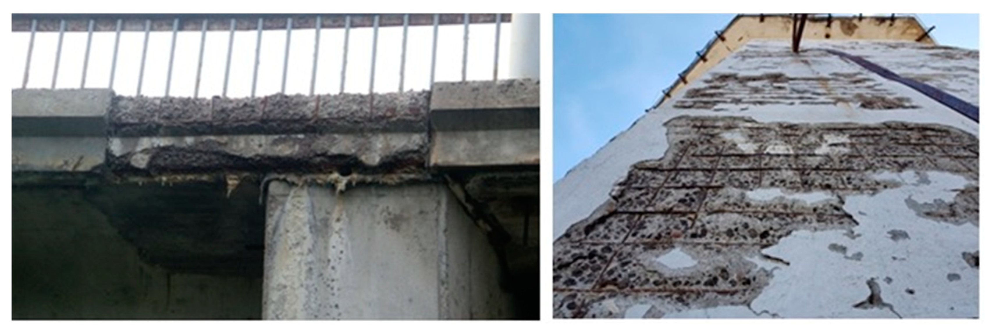
Figure 2.
Two-layered concrete specimen with gradually varied thickness of degraded upper layer ThD intended for ultrasonic surface scanning using three frequencies F1-F3
Figure 2.
Two-layered concrete specimen with gradually varied thickness of degraded upper layer ThD intended for ultrasonic surface scanning using three frequencies F1-F3
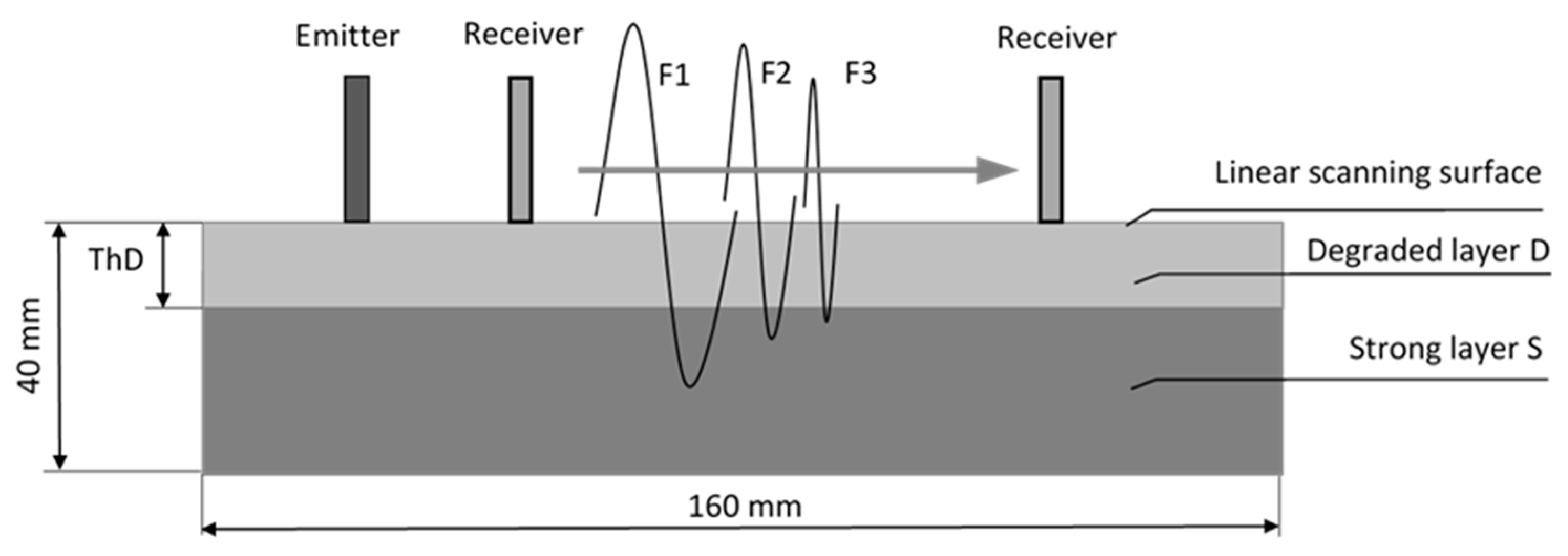
Figure 3.
Ultrasonic scanner in action: 1 – emitting transducer; 2 – receiving transducer; 3 – vertical position controls; 4 – linear displacement drive; 5 – PCB for scanning control; 6 – ultrasonic acquisition unit; 7 – double-layered concrete specimen. Vertical arrows show attachment of transducers; horizontal line shows the direction of step-by-step linear displacement of the receiving transducer
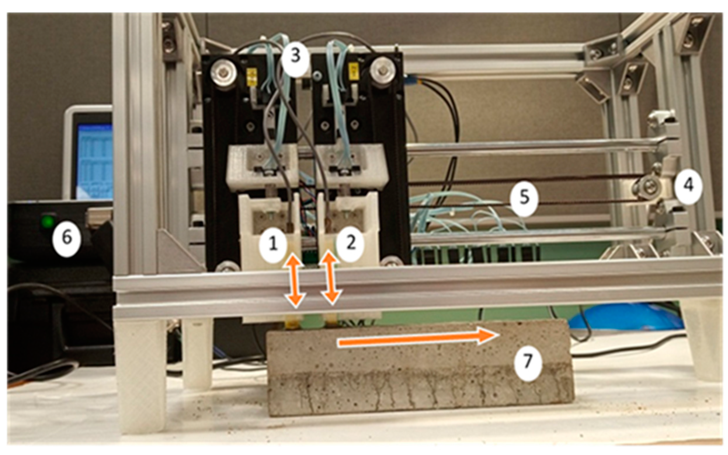
Figure 4.
Principal diagram of ultrasonic acquisition circuitry.
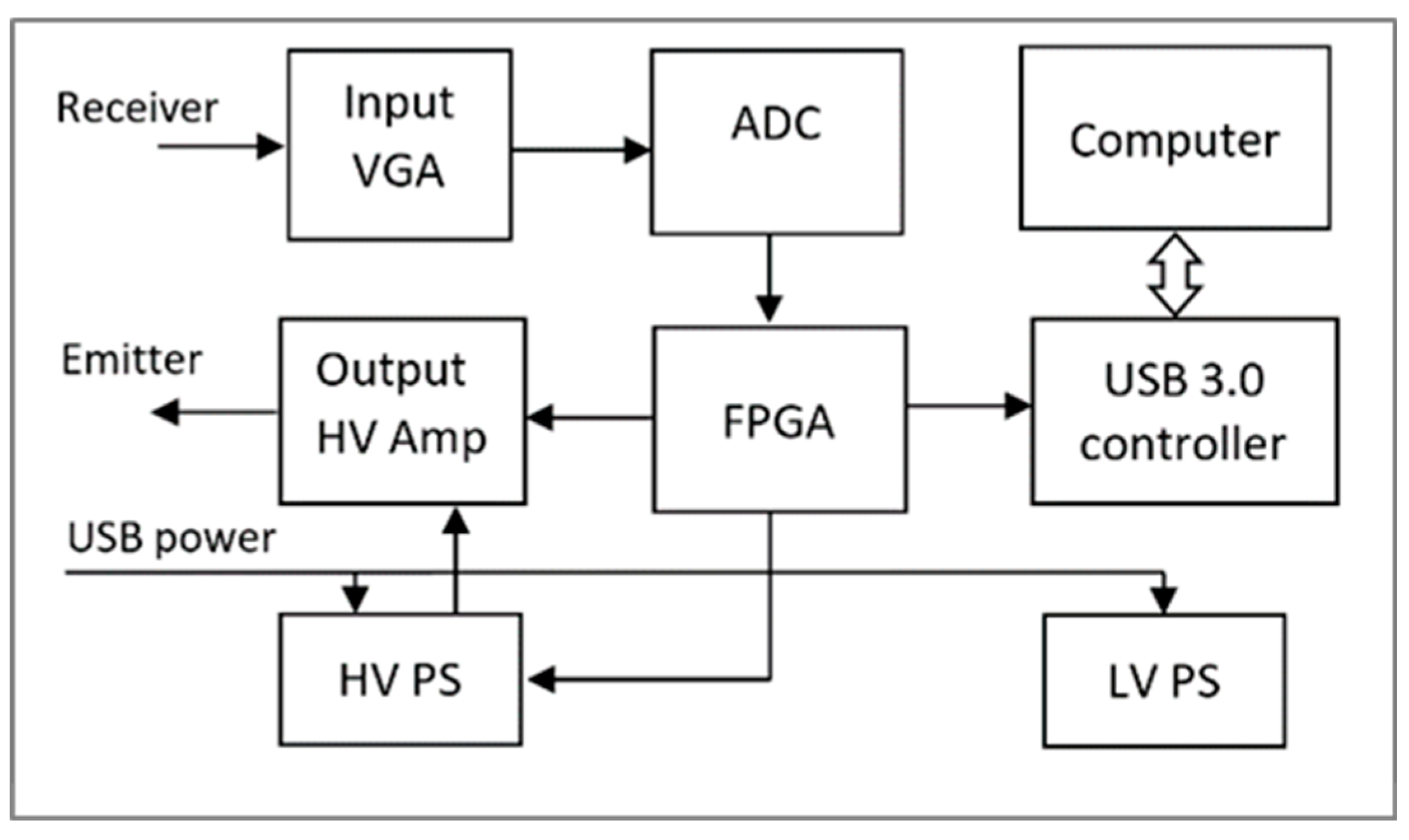
Figure 5.
NN architecture.
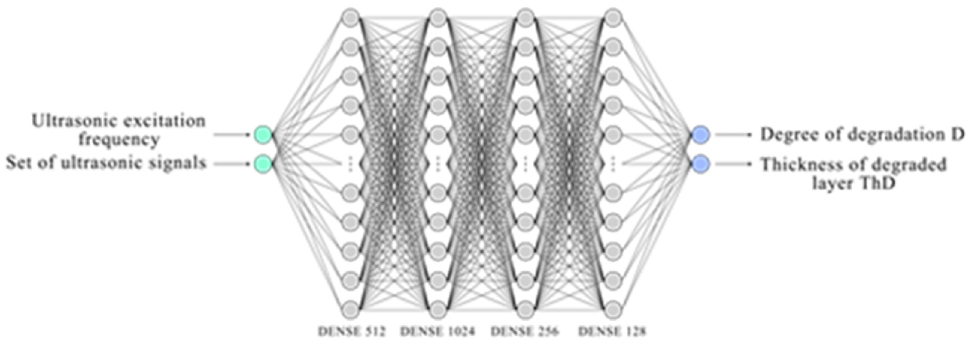
Figure 6.
Structure of dataset: black circles represent specimens for training and validation, empty circles represent specimens for testing
Figure 6.
Structure of dataset: black circles represent specimens for training and validation, empty circles represent specimens for testing
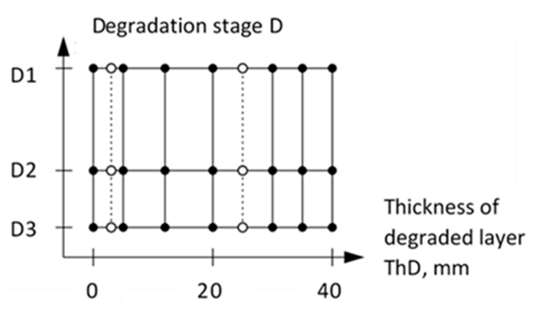
Figure 7.
Typical ultrasonic signals in a concrete specimen at 50, 100, and 200 kHz (left column) and spatiotemporal waveform profiles formed by step-by-step profiling of the specimen’s surface (right column).
Figure 7.
Typical ultrasonic signals in a concrete specimen at 50, 100, and 200 kHz (left column) and spatiotemporal waveform profiles formed by step-by-step profiling of the specimen’s surface (right column).
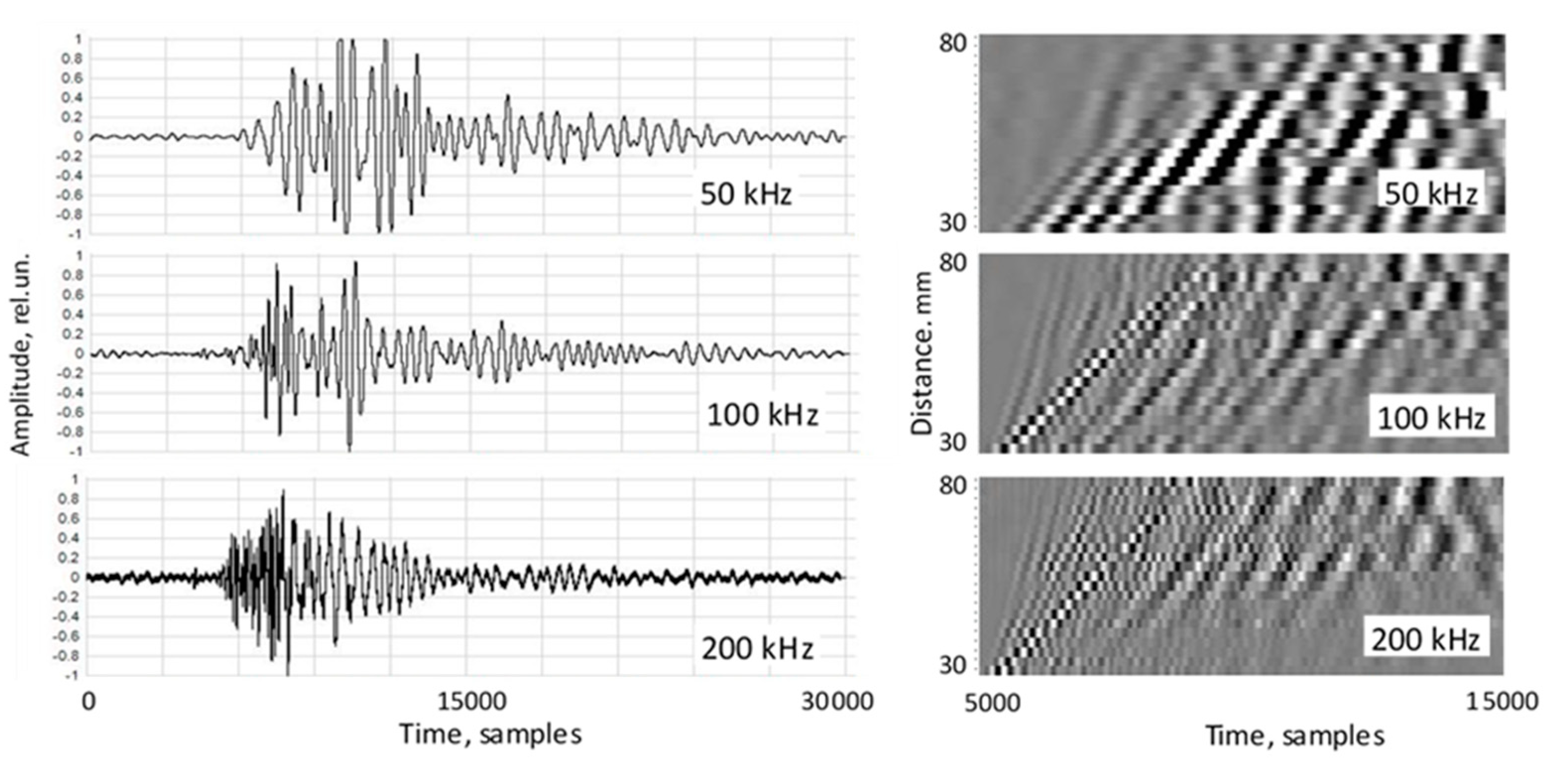
Figure 8.
Changes of spatiotemporal waveform profiles at 100 kHz with gradual increase of thickness of degraded layer ThD in specimens from the series with degradation degree D3: 1, 2 – wave front lines at ThD=0 mm and ThD=40 mm, correspondingly.
Figure 8.
Changes of spatiotemporal waveform profiles at 100 kHz with gradual increase of thickness of degraded layer ThD in specimens from the series with degradation degree D3: 1, 2 – wave front lines at ThD=0 mm and ThD=40 mm, correspondingly.
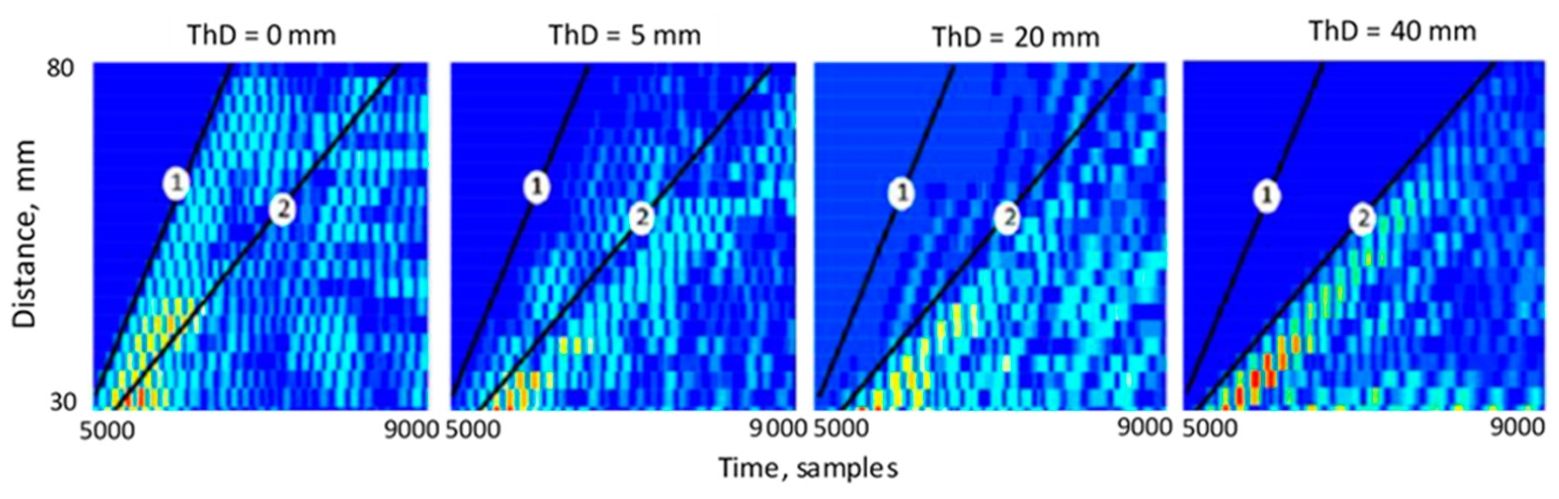
Figure 9.
Maximale for 3 degrees of deterioration relative errors for ThD.
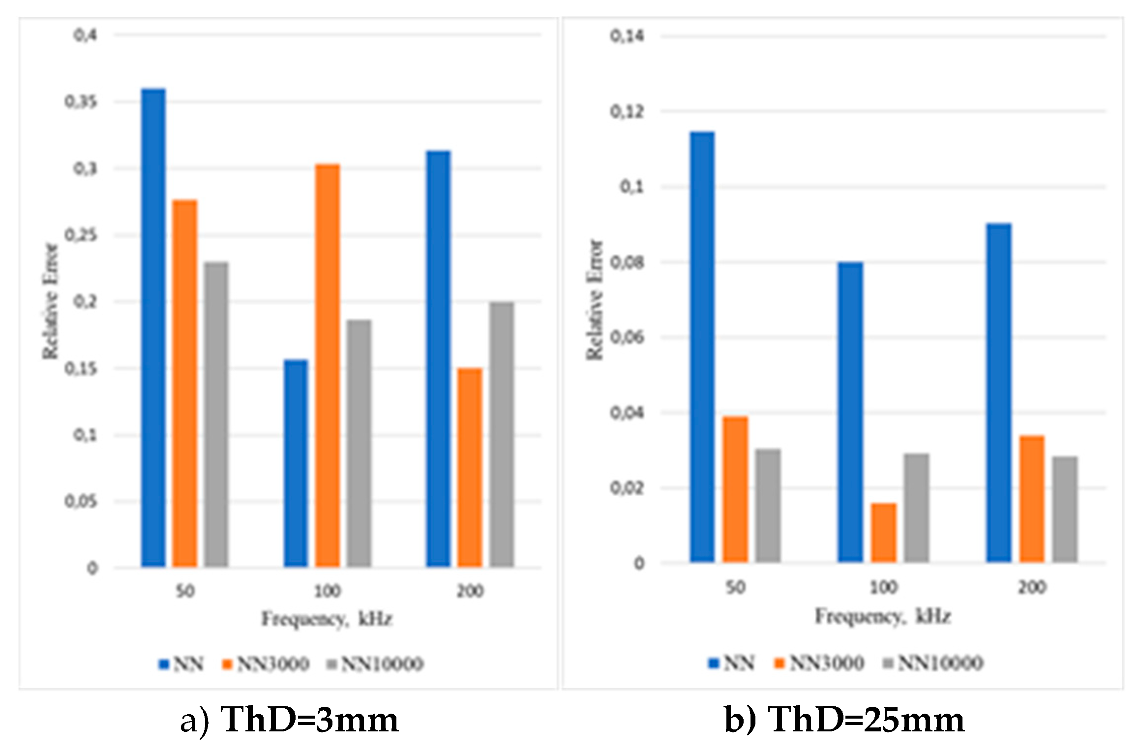
Figure 10.
Maximale for 3 degrees of deterioration relative errors for ThD.
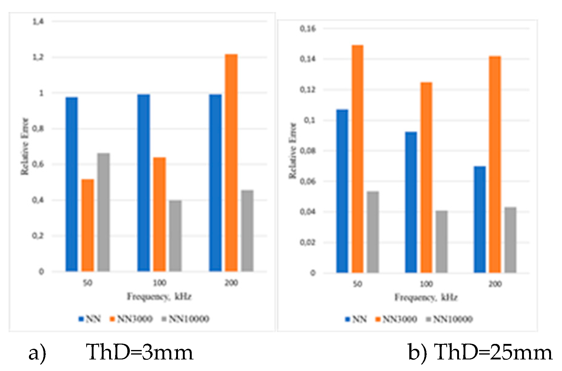
Figure 11.
Spectra of typical ultrasonic signals at carrier excitation frequencies 50, 100, and.200 kHz obtained by FFT: 1 – using cut signal length as for “NN10000” analysis; 2 – using entire signal length as for “NN” analysis; 3 – carrier excitation frequency.
Figure 11.
Spectra of typical ultrasonic signals at carrier excitation frequencies 50, 100, and.200 kHz obtained by FFT: 1 – using cut signal length as for “NN10000” analysis; 2 – using entire signal length as for “NN” analysis; 3 – carrier excitation frequency.
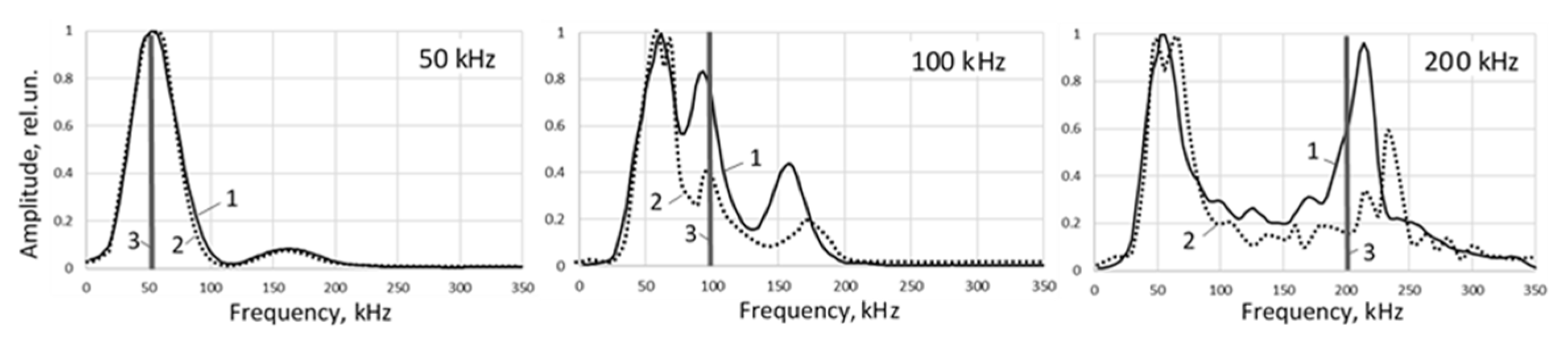

Table 1.
Parameters of ultrasonic acquisition.
| Parameter | Value |
|---|---|
| Applied ultrasonic frequencies | 50, 100, 200 kHz |
| Excitation waveform | 2-period sine tone-burst |
| Output voltage | 100 V p-t-p |
| ADC of received ultrasonic signals | 10-bit, 30 MHz |
| Length and step of scanning | 100 mm, 5 mm |
| Number of ultrasonic signals in a profile set | 21 |
Table 2.
Velocities of surface wave in monolithic specimens of S and D layers.
| Ultrasonic frequency, kHz | Velocity, m/s | |||
|---|---|---|---|---|
| S | D1 | D2 | D3 | |
| 50 | 2287 | 1916 | 1676 | 1266 |
| 100 | 2300 | 1978 | 1784 | 1278 |
| 200 | 2353 | 2020 | 1780 | 1318 |
Table 3.
Classification statistics for the applied network.
| Utrasonic frequency, kHz | Projected values | Predicted values with different networks | ||||||
|---|---|---|---|---|---|---|---|---|
| “NN” | “NN3000” | “NN10000” | ||||||
| D, degree | ThD, mm | D, degree | ThD, mm | D, degree | ThD, mm | D, degree | ThD, mm | |
| 50 | D1 | 3.0 | D3** | 3.67 | D1 | 2.31 | D1 | 3.69 |
| 50 | D2 | 3.0 | D2 | 4.08 | D2 | 3.83 | D2 | 3.09 |
| 50 | D3 | 3.0 | D1** | 3.99 | D3 | 2.91 | D3 | 2.44 |
| 100 | D1 | 3.0 | D1 | 3.34 | D1 | 2.36 | D1 | 3.50 |
| 100 | D2 | 3.0 | D2 | 3.44 | D2 | 2.60 | D2 | 3.56 |
| 100 | D3 | 3.0 | D3 | 2.53 | D3 | 3.91 | D3 | 3.06 |
| 200 | D1 | 3.0 | D1 | 2.84 | D1 | 3.40 | D1 | 2.80 |
| 200 | D2 | 3.0 | D2 | 3.94 | D2 | 3.45 | D2 | 2.84 |
| 200 | D3 | 3.0 | D3 | 2.94 | D3 | 3.40 | D3 | 3.60 |
| 50 | D1 | 25.0 | D1 | 23.64 | D1 | 25.98 | D1 | 25.65 |
| 50 | D2 | 25.0 | D2 | 25.32 | D2 | 24.99 | D2 | 24.63 |
| 50 | D3 | 25.0 | D3 | 27.87 | D3 | 25.73 | D3 | 25.76 |
| 100 | D1 | 25.0 | D1 | 26.44 | D1 | 24.60 | D1 | 24.84 |
| 100 | D2 | 25.0 | D2 | 27.00 | D2 | 25.04 | D2 | 24.27 |
| 100 | D3 | 25.0 | D3 | 25.67 | D3 | 25.34 | D3 | 24.50 |
| 200 | D1 | 25.0 | D1 | 27.26 | D1 | 25.85 | D1 | 25.19 |
| 200 | D2 | 25.0 | D2 | 27.09 | D2 | 25.66 | D2 | 25.42 |
| 200 | D3 | 25.0 | D3 | 24.70 | D3 | 24.53 | D3 | 24.29 |
**- deviation in D by 2 gradations
Table 4.
Classification statistics for the applied network.
| Utrasonic frequency,kHz | Projected values | Predicted values with different networks | |||||||
|---|---|---|---|---|---|---|---|---|---|
| “NNFT” | “NNFT3000” | “NNFT10000” | |||||||
| D, degree | ThD, mm | D, degree | ThD, mm | D, degree | ThD, mm | D, degree | ThD, mm | ||
| 50 | D1 | 3.0 | D2* | 0.99 | D3** | 3.92 | D1 | 4.99 | |
| 50 | D2 | 3.0 | D2 | 3.67 | D2 | 2.83 | D2 | 4.09 | |
| 50 | D3 | 3.0 | D1** | 5.93 | D3 | 4.55 | D3 | 1.37 | |
| 100 | D1 | 3.0 | D1 | 1.23 | D3** | 3.36 | D1 | 1.80 | |
| 100 | D2 | 3.0 | D3* | 0,024 | D3* | 4.34 | D2 | 1.87 | |
| 100 | D3 | 3.0 | D3 | 1.86 | D3 | 4.92 | D3 | 4.09 | |
| 200 | D1 | 3.0 | D1 | 3.95 | D3** | 6.65 | D1 | 2.19 | |
| 200 | D2 | 3.0 | D2 | 5.09 | D2 | 3.97 | D2 | 2.29 | |
| 200 | D3 | 3.0 | D2* | 5.98 | D3 | 4.87 | D2* | 4.37 | |
| 50 | D1 | 25.0 | D1 | 22.32 | D1 | 28.73 | D1 | 23.66 | |
| 50 | D2 | 25.0 | D3* | 22.89 | D2 | 27.47 | D3* | 25.00 | |
| 50 | D3 | 25.0 | D3 | 26.10 | D3 | 28.35 | D3 | 26.21 | |
| 100 | D1 | 25.0 | D1 | 24.91 | D1 | 26.88 | D1 | 23.98 | |
| 100 | D2 | 25.0 | D2 | 25.66 | D2 | 23.31 | D2 | 24.51 | |
| 100 | D3 | 25.0 | D1** | 22.69 | D3 | 28.12 | D1** | 24.55 | |
| 200 | D1 | 25.0 | D1 | 26.75 | D1 | 28.20 | D1 | 23.92 | |
| 200 | D2 | 25.0 | D2 | 23.42 | D2 | 28.55 | D2 | 24.47 | |
| 200 | D3 | 25.0 | D3 | 26.58 | D3 | 25.34 | D3 | 24.29 | |
*, **- deviation in D by 1 and 2 gradations, correspondingly.
Disclaimer/Publisher’s Note: The statements, opinions and data contained in all publications are solely those of the individual author(s) and contributor(s) and not of MDPI and/or the editor(s). MDPI and/or the editor(s) disclaim responsibility for any injury to people or property resulting from any ideas, methods, instructions or products referred to in the content. |
© 2024 by the authors. Licensee MDPI, Basel, Switzerland. This article is an open access article distributed under the terms and conditions of the Creative Commons Attribution (CC BY) license (http://creativecommons.org/licenses/by/4.0/).
Copyright: This open access article is published under a Creative Commons CC BY 4.0 license, which permit the free download, distribution, and reuse, provided that the author and preprint are cited in any reuse.


