
Submitted:
13 November 2024
Posted:
15 November 2024
You are already at the latest version
Abstract
This paper describes recent variations that have emerged in spatial patterns of retroflections in the monthly Gulf Stream (GS) path. They have become less frequent and also shifted further to the east; we find this in both reanalysis and free-running model data of the ocean. A suite of eddy-rich North Atlantic ocean ensemble simulations, forced with varying combinations of realistic and climatological boundary conditions, is used to diagnose the relative importance of atmospheric and oceanic drivers of these changes. It is implied that the majority of the shifts and changes in the number of retroflections throughout the five decades (1963-2012) are products of realistic atmospheric forcing and oceanic boundary conditions but only the latter is found to be statistically significant.
Keywords:
Gulf Stream
; Ensemble simulation
; Sea Surface Height
1. Introduction
The Gulf Stream (GS) constitutes a very important part of Earth’s ocean circulation. It is the western boundary current (WBC) of the North Atlantic (NA) subtropical gyre, transporting up to 150 Sv of warm waters from the tropics to the subpolar regions [1]. This in return affects Earth’s heat budget and influences the large-scale climate [2]. Despite decades of research having gone into GS, the study of its properties and how they change remains of importance. It has been documented that some of the GS properties may have changed over recent decades. For example, studies have reported that it is warming faster than the global ocean and shifting closer to the shore [3], which is known to impact the fishing industry [4]. Other examples include, the westward shift of the destabilization point [5,6], slow-down of the GS [7], shift in its position, speed and transport [8], or asymmetries in the warm and cold core GS eddy formation affecting the heat transfer in the region [9,10].
The property that we analyze in this study is the GS path. Recent work using satellite mapped mean sea level anomalies has revealed that after the point of separation from the U.S. coast near Cape Hatteras, the GS path exhibits two leading modes of variability: Meridional shifts and large-amplitude GS meanders [11]. These lateral shifts or low-frequency meridional movements in the position of the Gulf Stream path have been demonstrated to be product of oceanic processes such as baroclinic oceanic Rossby waves propagating westward [12], the influence of El Niño Southern Oscillation (ENSO) in the North Atlantic [13,14], reversals in the Atlantic Meridional Overturning Circulation AMOC [15], or changes in the atmosphere, for example, the response to wind curl variability associated with the North Atlantic Oscillation NAO [16,17]. These changes in GS have been further argued to influence the atmosphere. The work by Kwon and Joyce [18] showed that the extension and intensity of the NA storm track is sensitive to the meridional position of the GS. More recently, it was found that meridional shifts in the GS path are associated with deviations of the storm track to the northeast over the Labrador Sea and a reduction or enhancement in Greenland blocking [19]. Nevertheless, an emphasis in statistical details on large longitudinal changes in the GS path have not garnered adequate attention. Here, we are interested in the meandering nature of the GS paying attention to significant deviations of the GS trajectory. We shall refer to these as GS retroflections (cf. Figure 1a).
The nature of these retroflections can potentially impact the location of the GS temperature front. Thus, changing the spatial distribution of the regional sea-surface temperature (SST) and hence the gradient field. This is important because the strong GS SST gradient impacts the atmosphere on different scales. At scales greater than 100 km, differential heat fluxes induced by the strong SST gradient can act as a major restorative force for surface baroclinicity destroyed by the passage of strong atmospheric storm systems (via oceanic baroclinic adjustment) [20,21], effectively anchoring the mid-latitude storm-tracks [22]. At finer scales, these differential heat fluxes can also directly impact atmospheric fronts embedded within these storms [23,24], which can contribute up to 90% of the precipitation across the Euro-Atlantic sector [25]. In this manner, the effective SST gradient that an atmospheric front propagating across the GS will experience depends both on the local SST gradient as well as the “waviness” of the GS path. The latter will be impacted strongly by GS retroflections. Therefore, understanding how these have changed through time and their characteristics might be of interest for the air-sea interaction setting
Accordingly, the objective of this paper is to document how GS retroflections have changed over the last decades. Section 2 describes the data and methods used in this study. Section 3 examines the trends in GS retroflections in reanalysis, as well as in a suite of ocean ensemble models. We end with a Discussion in Section 4.
2. Data and Methods
Sea-surface data from the European Centre for Medium-Range Weather Forecasts (ECMWF) is used, specifically the Ocean Reanalysis System 5 ORAS5 [26] from 1963 to 2012. The variables used to identify the Gulf Stream (GS) are sea-surface height (SSH) and surface meridional and zonal velocities. The operational system OCEAN5 is used with a Behind-Real-Time component to provide an estimate from 1958 to present (with a few days of delay) and a Real-Time component for the latest ocean conditions. The model resolution in OCEAN5 is 1/4° in the horizontal and 75 levels in the vertical, improving the previous system, OCEAN4, with a new generic ensemble generation scheme [27] that accounts for both observational and forcing errors. ORAS5 uses Mercator coordinate grids south of the Arctic, and monthly temporal resolution. Therefore, the GS paths analyzed here represent the monthly mean for each specific year.
To further investigate the relative importance of atmospheric and oceanic drivers, a suite of eddy-rich (1/12°) ocean model ensembles of the North Atlantic (20°S-55°N) is examined using the Massachusetts Institute of Technology general circulation model MITgcm [28]. The same model outputs have been used to study the spatiotemporal characteristics of AMOC [29,30,31] and eddy-mean flow interactions [32,33,34]. The suite of ensembles are subject to various combinations of climatological and realistic forcings. The Ocean-Realistic, Atmosphere-Realistic (ORAR) simulations, which are the most realistic, prescribe full atmospheric variability and fully variable open ocean boundary conditions at the northern and southern boundaries and Strait of Gibraltar for the 50 years of 1963-2012. Other combinations include a climatological atmospheric state with fully varying open ocean boundary conditions (Ocean-Realistic, Atmosphere-Climatology; ORAC), fully varying atmosphere and climatological open ocean boundary conditions (Ocean-Climatology, Atmosphere-Realistic; OCAR) and climatological forcing conditions of all types (Ocean-Climatology, Atmosphere-Climatology; OCAC). Runs with a climatological boundary condition are subject to a “repeating year” whereby the atmospheric forcing and oceanic boundary conditions repeat the July 1, 2002 to June 30, 2003 conditions [30]. This year was chosen specifically as it was both relatively neutral with regards to NAO and ENSO, and the choice to repeat from summer to summer was to limit any impacts of a jump in the summertime mixed layer depth, which is shallow relative to that in winter. The entire set of ensembles consists of 24 members of ORAR, 12 members of ORAC, 12 members of OCAR, and 24 members of OCAC.
3. Results
3.1. Trend in Retroflection Patterns
The GS path characteristics can be described using a SSH isoline that follows the GS jet [5,6,35,36]. However, after the point of separation from the east coast of the USA, the Gulf Stream flows downstream having two recirculation pathways after approximately 55°W e.g. Figure 1a [37,38]. The interaction with the northern recirculation gyre (NRG) leads to a flow moving northward whereas a southward flow joins the so-called Worthington Gyre (WG). This bifurcation plus the meandering nature of the GS increase the variability of the GS path making it difficult to identify the path using just one isoline of SSH. Therefore, we examined a range of different SSH contours covering heights from −25 cm to 3 cm. These values showed very good agreement with the maximum of the SSH gradient up to 55°W (Figure A1). After this point, some of these isolines captured the northern trajectory and others the southern trajectory followed by the GS when recirculating. This identification might include closed contours that describe eddies, so, in order to avoid that, only the longest continuous contour is taken into account. We also examined the 25 cm isoline, which is the contour used by other studies [5,6,35,36], but this yielded contours local to the Straits of Florida. This discrepancy in the contour values likely has to do with whether the geoid is excluded or not from SSH. Figure 1b displays the mean over the 50-year record of the GS path and its variability for the −11 cm SSH isoline using the reanalysis product. The −11 cm isoline is the most southern isoline within a reasonable range of latitudes that captures the temporal shift in Gulf Stream retroflection patterns (Figures 1b and A3).
A retroflection will be defined as the first segment of the GS path where the overall eastward trajectory followed by the jet deflects westward for more than 260 km (~3° in longitude; e.g. green curve in Figure 1a). In other words, the length along the portion of the deflected trajectory to the west has to be longer than 260 km. In this sense, our definition of a retroflection is different from the ones used in other WBC circulation systems such as the Agulhas Current in the Southern Hemisphere where a retroflection is an extension of the current when separating from the shore [39]. The length of 260 km was set to ensure that the change in the Gulf Stream path was significantly greater than the average wavelength of GS meanders [40].
Each GS path is represented by two vectors of the same length, one containing the longitude and the other the latitude of each point in the path. To identify the retroflections we take the difference of the longitude vector for each GS path. The portions of the trajectory where this difference is negative represents a westward deflection and therefore it gives a suitable candidate for a retroflection. Then, the length along each of those segments is calculated. The first segment that is more than 260 km long is a retroflection and where it begins (i.e. its most eastward longitude) is saved.
The 50-year (1963-2012) record of reanalysis and ensemble simulations used in this paper is divided in two periods covering the first 25 years (1963-1987) and the latter 25 years (1988-2012) of data. This division was suggested by a first look at the ensemble results from the most realistic simulation (ORAR) where there was a distinct difference in the GS path length between these two periods (Figure 2a) when calculating it between 75°W and 50°W. This zonal range was initially chosen to be consistent with previous studies examining GS paths [5,6]. The −11 cm SSH isoline from the ORAS5 reanalysis is shown along with the 25 cm isolines from the four ensemble outputs (Figure 1b). As was also noted earlier, the choice of the 25 cm isoline of SSH is consistent with previous studies [5,6,35,36] and is in line with the behavior and variability of the one exhibited by the ORAS5 product (Figure 1b).
The time series in Figure 2 generally exhibit heightened temporal variability for the GS path length during the first 25 years when the analysis is confined between 75°W-50°W. However, the path lengths demonstrate no obvious temporal trend when analyzed over the entire North Atlantic zonal extent; this suggests that the retroflections have shifted further eastward of 50°W. We also find that the path lengths are significantly shorter in the ensemble mean than in ORAS5 (Figure 2f); this has to do with the fact that the ensemble-mean paths have fewer meanderings than a single realization particularly eastward of 50°W. Nonetheless, the transition in temporal variability is still observed in the ensemble mean of ORAR.
The histograms in Figure 3 describe the longitude of the first retroflection as a function of its relative probability for both of the periods. The relative probability is simply the ratio between the number of retroflections found in a 1° bin divided by the total amount of retroflections across all bins. A probability density function (PDF) is fit to each histogram using the fitdist and pdf functions in MATLAB and its first four central moments (mean, variance, skewness and kurtosis) are calculated. To see if the distributions for each period are actually different, the Kolmogorov-Smirnov test to the 95% confidence level between them was performed [41]. These results showed that from the range of SSH contours taken, only the interval from −25 cm to −11 cm proved to be statistically significant in distinguishing the PDFs (Figure A3). Namely, there is a distinction in the number of retroflections between the two periods with it being greater in the first 25 years. This is present in almost all the analyzed contours except in the −25 cm (Figure A2). It is worth noting that this specific isoline lies at the edge of the regime where the GS interacts with the NRG so this difference may be a product of this northward tendency of the flow. There is an eastward shift in the mean of the distribution of the first period (45°W) with respect to the second period (40°W) and the occurrence of retroflections becomes less frequent. This feature is captured by all of the other analyzed SSH contours (Figure A2). Looking at the other moments we see that the skewness and kurtosis are greater in the first period whereas the variance is greater in the second period meaning that the PDF is wider (Figure 3). It has to be noted that there is no clear pattern for skewness and kurtosis as they vary depending on the chosen contour (Figure A2). The retroflections appear to be more present east of 50°W peaking at around 40°W (Figures 3 and A2).
3.2. Potential Causes for the Retroflection Trend
We now examine our suite of North Atlantic simulations to investigate the potential driver of these retroflections. The ensemble mean of these simulations is used to better capture the oceanic response to the forcing of the system and minimize the signal of intrinsic variability present in each individual member. The resulting histograms for each of the four experiments are included in Figure 4. Similar to the ORAS5 case, the Kolmogorov-Smirnov test to the 95% confidence level was performed on the PDFs; the results are shown in Figure A4.
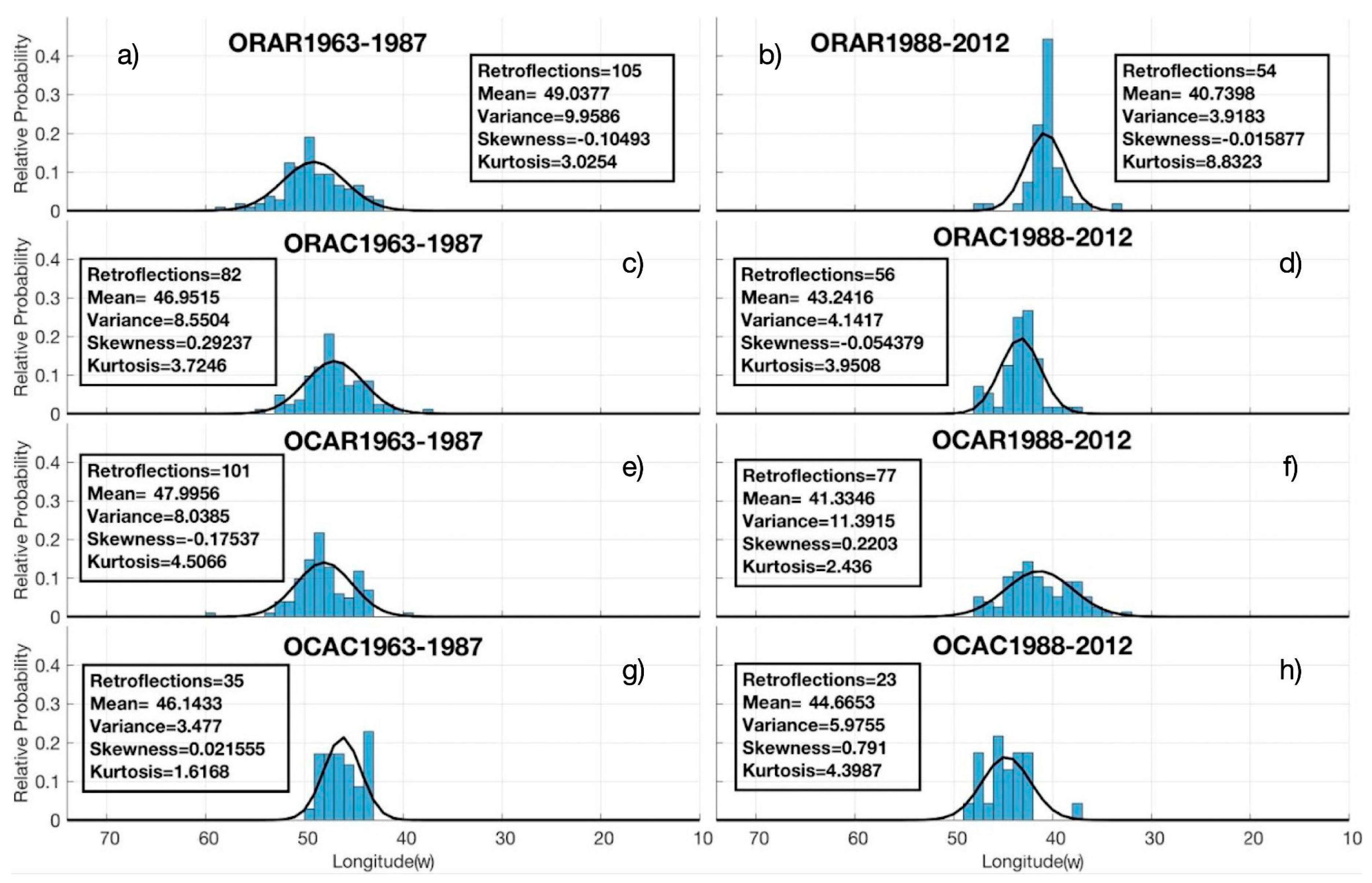
Each group of simulations provides a different perspective; for instance, the ensemble mean of ORAR represents the ocean response to a fully forced system capturing the most realistic oceanic and atmospheric variability in the boundary conditions and forcing. The ensemble mean of ORAC captures the response to an atmosphere fixed for the year of 2002 and fully varying oceanic boundary conditions. In the OCAR ensemble, the results will describe the retroflections in the presence of a realistic atmosphere interacting with an ocean with climatological boundaries of 2002. Lastly, OCAC depicts the oceanic response to the climatological boundary conditions and forcing specific to the repeating year of 2002. The fact that the mean path and variability about it remain similar amongst the ensembles (Figure 1b) permits us to intercompare them and suggest the driving factor in the shift of retroflections.
When oceanic boundary conditions are realistic in the simulations (ORAR and ORAC; Figure 4a-d), we see that the PDFs are wider in the first period and narrower in the second with a statistically significant eastward shift in the retroflections and fewer of them occurring in the second half. While there is also a shift in the mean of the PDF in OCAR (Figure 4e,f), the two PDFs are not statistically distinct from each other based on the Kolmogorov-Smirnov test (Figure A4). If both, the oceanic boundary conditions and prescribed atmosphere, are climatological (OCAC; Figure 4g,h), a large decrease in the number of retroflections and in the variance for the first period is observed (see variance in Figure 4g). In the OCAC case, the variance for the first and second half of the 50-year period is comparable; namely, their difference is ~2.5°, the smallest amongst all realizations, meaning that the two histograms are confined to a narrow range of longitudes (Figure 4g,h). What these differences between the ensembles demonstrate is that the realistic oceanic boundary conditions make the PDFs narrower over time whereas they become wider with realistic atmospheric forcing. One can corroborate this by looking at the change in variance for ORAR, ORAC and OCAR.
4. Conclusions and Discussion
This study presents the analysis of a very particular feature of the Gulf Stream (GS), namely westward deflections of its trajectory, called retroflections (Figure 1). Fifty years of reanalysis and ensemble simulation data were used to detect the GS path and its retroflections. Reanalysis data revealed that there is a clear distinction between the first and second half of the record; during the first half, the number of retroflections appears to be greater and contained to the west relative to the second half (Figure 2 and Figure 3). These results are relatively insensitive to the specific SSH isoline (Appendix A) and are consistent with observational data over recent decades that have exhibited a shift in the GS path and rings shed from it [6,9,10].
The importance of these findings are of potential interest from an air-sea interaction perspective given the tight relation between the GS and its impact on the atmosphere. The appearance of a retroflection can potentially modify the disposition of the GS front affecting the location of the surface heat fluxes from the ocean to the atmosphere and SST gradient. As such, tropical cyclones and atmospheric fronts might be affected by changes in the behavior of GS retroflections [42], since the evolution and frequency of these types of systems are sensitive to the location and sharpness of the SST gradients [43]. The specific impact of GS retroflections and their trend on altering the storm tracks and low-pressure systems will be left for future study.
Further analysis with a set of ocean model ensemble experiments unraveled that in the absence of a realistic oceanic boundary condition and atmospheric forcing: i) these retroflections did not significantly reduce in their number, and ii) there was no longer a noticeable eastward shift in the longitudes where they appear in the second period with respect to the first period (Figure 4). A composite mean of wind and SST anomalies when retroflections were detected were calculated between each halve of the ensemble outputs (Appendix B). As one may expect, there is the least amount of difference between the two periods in the OCAC case (Figure B1). The differences in Figure B1 amongst the ensemble experiments should not be interpreted as the definitive cause for the eastward shift or the reduction in number of the GS retroflections from the first half to the latter but, rather as the model pointing to the fact that the oceanic and atmospheric circulation patterns associated with retroflections have non-trivially altered over the five decades. This is a good motivation for future and different research avenues. One might be to test the actual response of atmospheric systems to the appearance of these retroflections and quantify the change of heat fluxes and the meridional SST gradient along the separated and retroflected GS versus the response to a less “wavy” GS. Relating the NAO and ENSO indices to the timing of retroflections may also be of potential interest [8,14,16]. Another avenue may be to examine whether the heat and salt transport associated with AMOC or through the Strait of Gibraltar have exhibited any significant trends in affecting the large-scale stratification of the North Atlantic [44,45]. The lanes that one can take are endless since very little is known about variability in GS retroflections; the main goal of the present work was to open the conversation and exploration around it.
Acknowledgements
This study is a contribution to the ‘Assessing the Role of forced and internal Variability for the Ocean and climate Response in a changing climate’ (ARVOR) project supported by the French ‘Les Enveloppes Fluides et l’Environnement’ (LEFE) program. W. Dewar is supported through National Science Foundation (NSF) grants OCE-1829856, OCE-1941963, and the French ‘Make Our Planet Great Again’ (MOPGA) program managed by the Agence Nationale de la Recherche under the Programme d'Investissement d'Avenir, reference ANR-18-MPGA-0002. Dewar, R. Parfitt and T. Uchida acknowledge support from the NSF grant OCE-2123632. Dewar and Parfitt acknowledge additional support from the NSF grant OCE-2023585. Parfitt also acknowledges NERC through Grant Ref: NE/V014897/1 and the NOAA Climate Variability and Predictability Program (NA22OAR4310617). High-performance computing resources on Cheyenne (doi:10.5065/D6RX99HX) used for running the Chaocean ensemble of the North Atlantic were provided by NCAR's Computational and Information Systems Laboratory, sponsored by NSF, under the university large allocation UFSU0011. We would like to extend our gratitude to Edward Peirce and Kelly Hirai for maintaining the Florida State University cluster on which the data were analyzed.
Appendix A. Sensitivity to the SSH Isoline
The range of isolines corresponding to the mean SSH are displayed in Figure A1. We provide the histograms and PDFs of the longitude associated with GS retroflections from ORAS5 when the SSH isolines range from −25 cm to 3 cm with 1 cm increments (Figure A2). There is a general tendency for the PDFs to shift westward with an increase in isolines. Figure A3 provides the Kolmogorov-Smirnov test at the 95% confidence level for the PDFs documented in Figure A2. The test results for the four ensemble experiments are given in Figure A4.
Figure A1.
The range of ORAS5 SSH contours examined in this study ([−25,3] cm) are presented in white curves. The −11 cm isoline adopted in the main text is shown in the black curve. The shading represents the magnitude of the mean SSH gradient calculated over the whole 50 years of record.
Figure A1.
The range of ORAS5 SSH contours examined in this study ([−25,3] cm) are presented in white curves. The −11 cm isoline adopted in the main text is shown in the black curve. The shading represents the magnitude of the mean SSH gradient calculated over the whole 50 years of record.
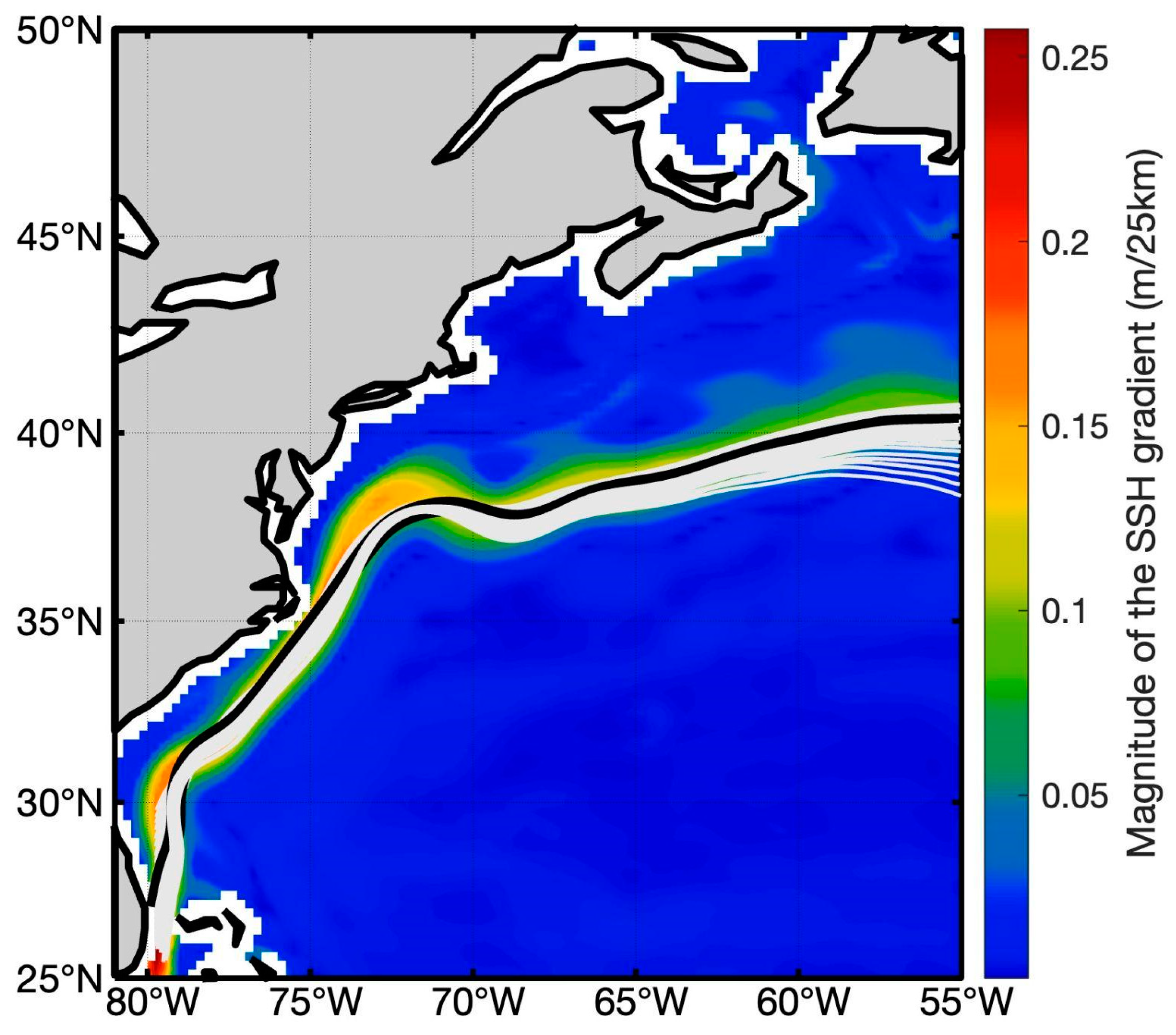
Figure A2.
Histograms of the longitude of GS retroflections from ORAS5 using SSH isolines ranging between −25 cm and 3 cm with 1 cm increments.
Figure A2.
Histograms of the longitude of GS retroflections from ORAS5 using SSH isolines ranging between −25 cm and 3 cm with 1 cm increments.
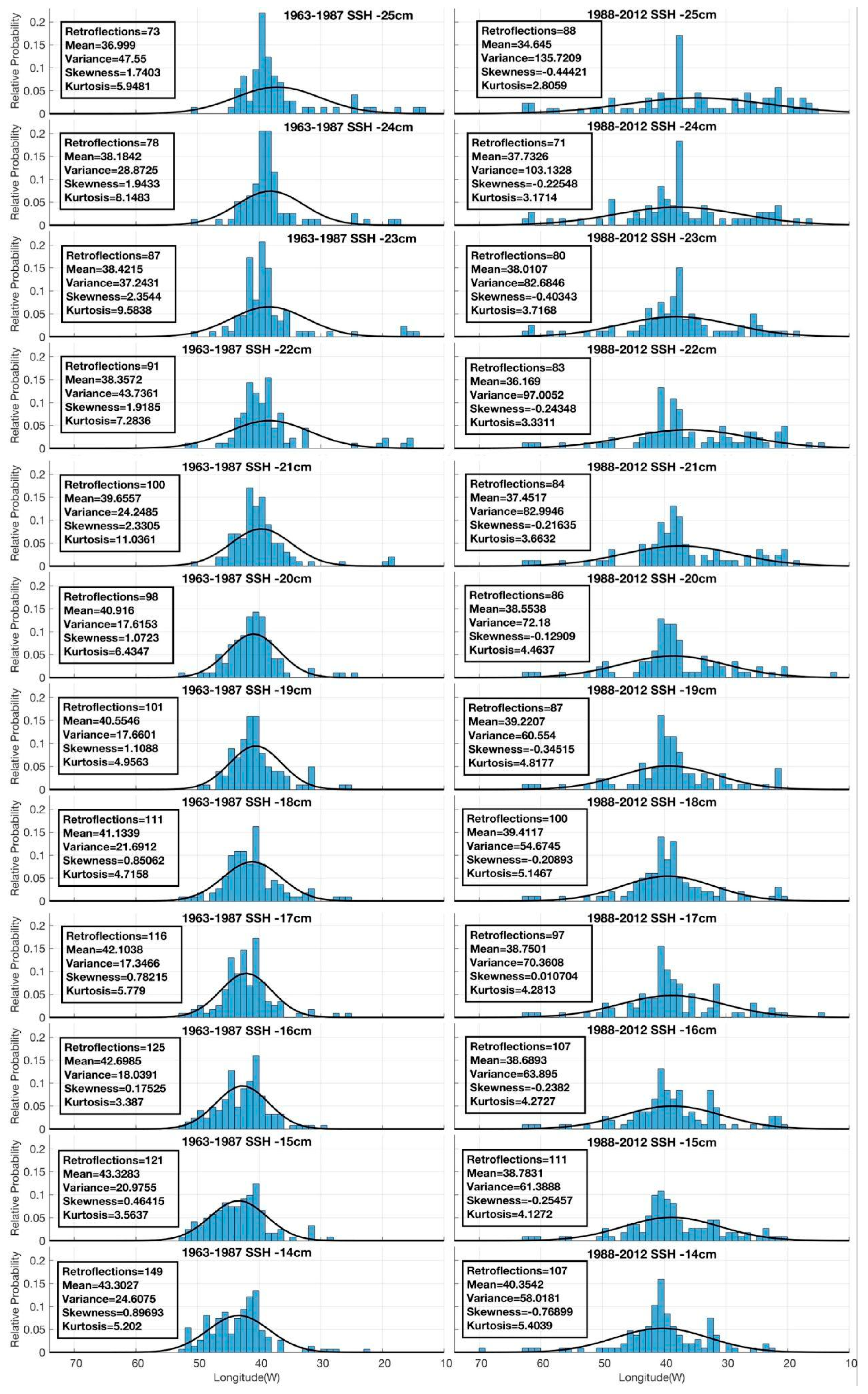
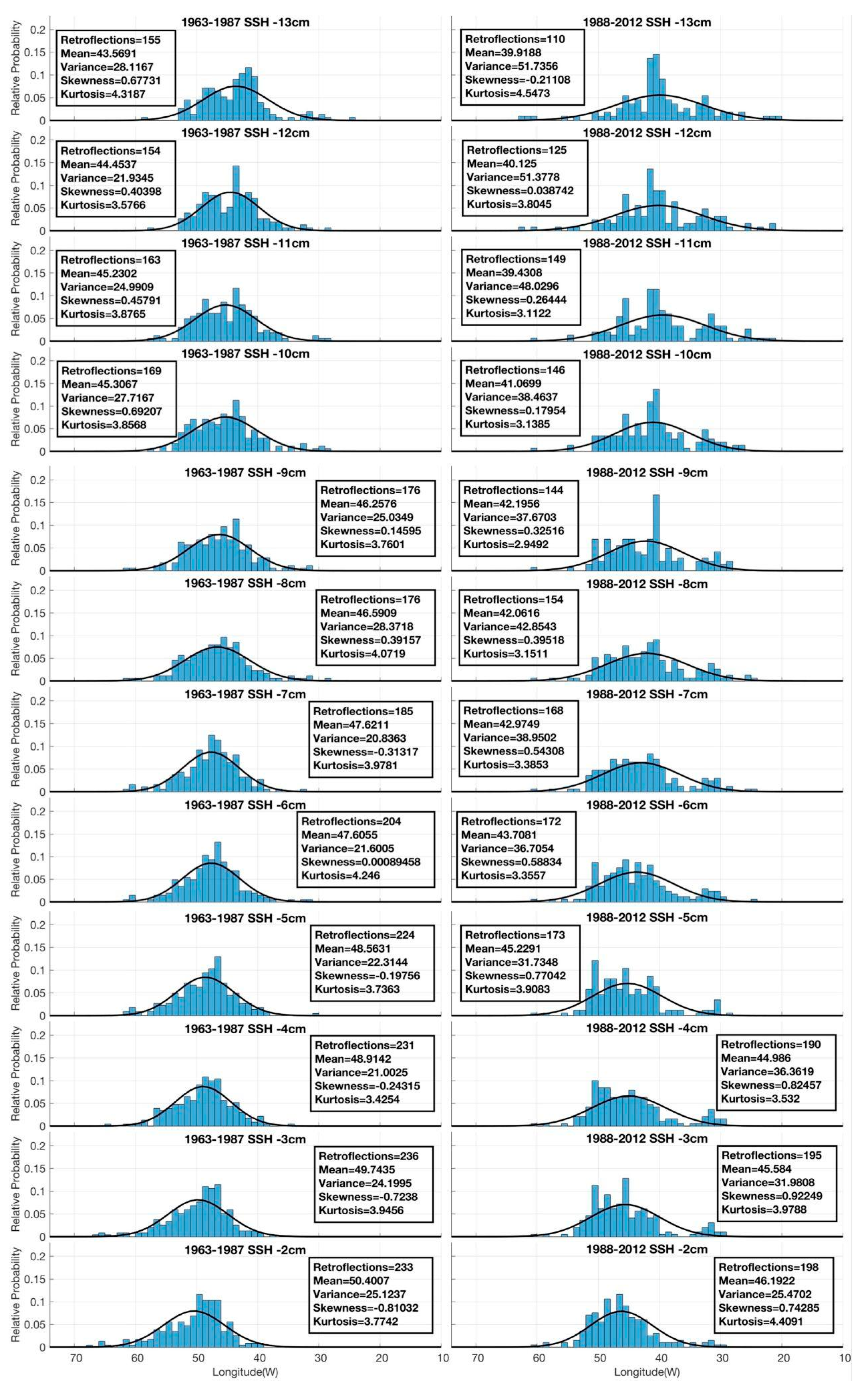
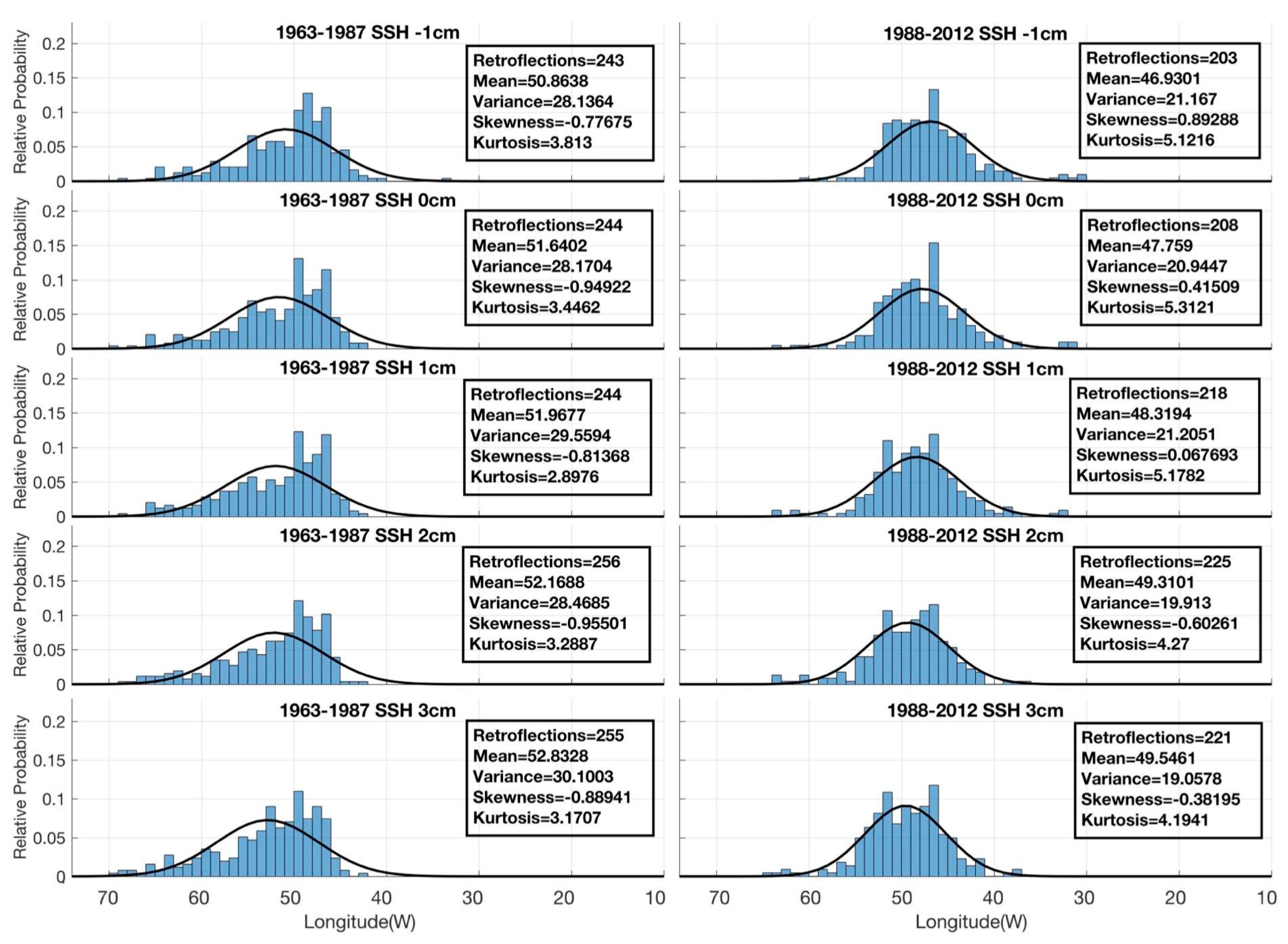
Figure A3.
Bar chart showing the results of the Kolmogorov-Smirnov test for the different SSH contours chosen from the ORAS5 dataset. The y axis documents the test result to the null hypothesis that the distribution from each half of the record comes from the same normal distribution; 1 means a rejection of the null hypothesis and 0 means that it cannot be rejected to the 95% confidence level.
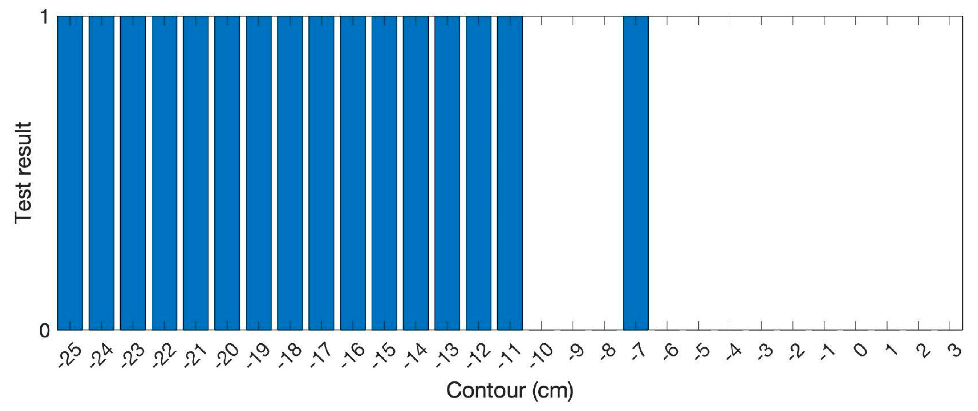
Figure A4.
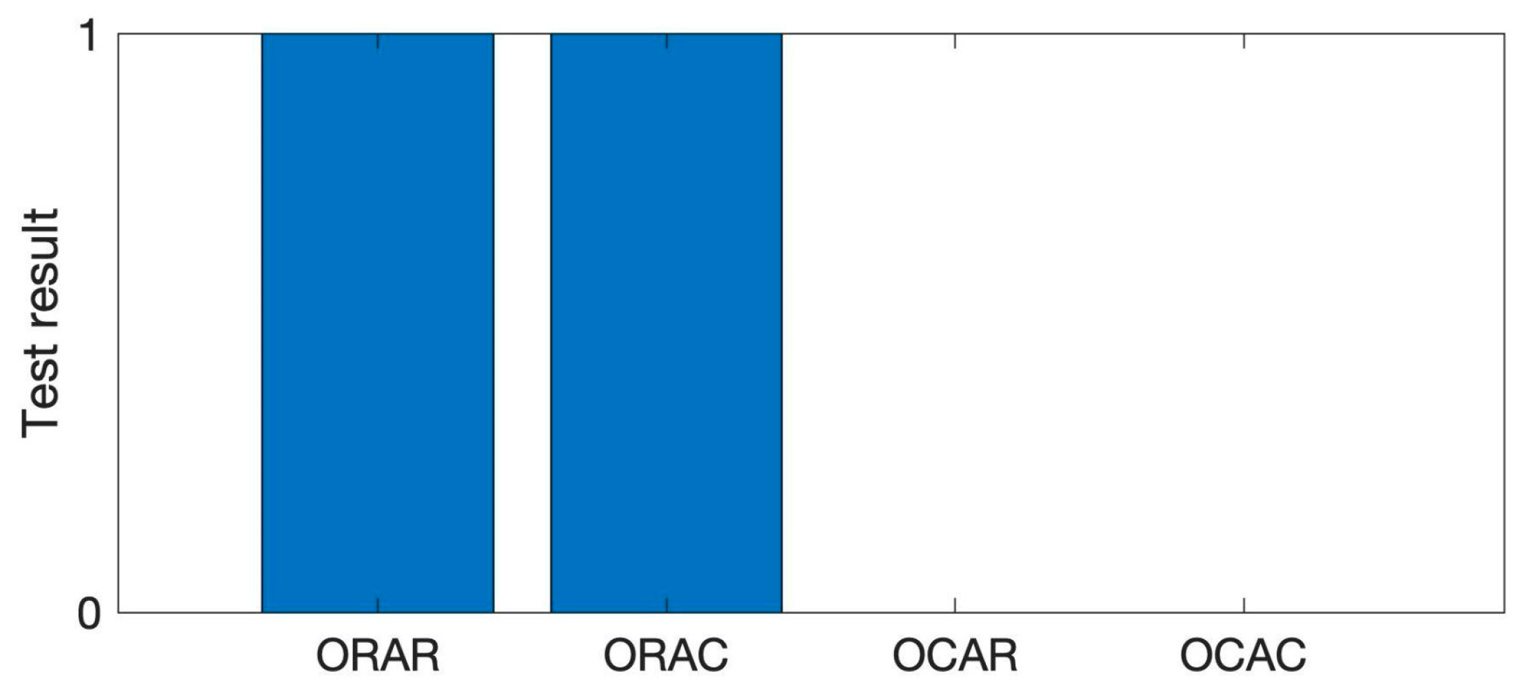
Same as Figure A3 but for the four ensemble experiments.
Figure A4.
Same as Figure A3 but for the four ensemble experiments.
Appendix B. Composite Mean of Wind and SST Anomalies
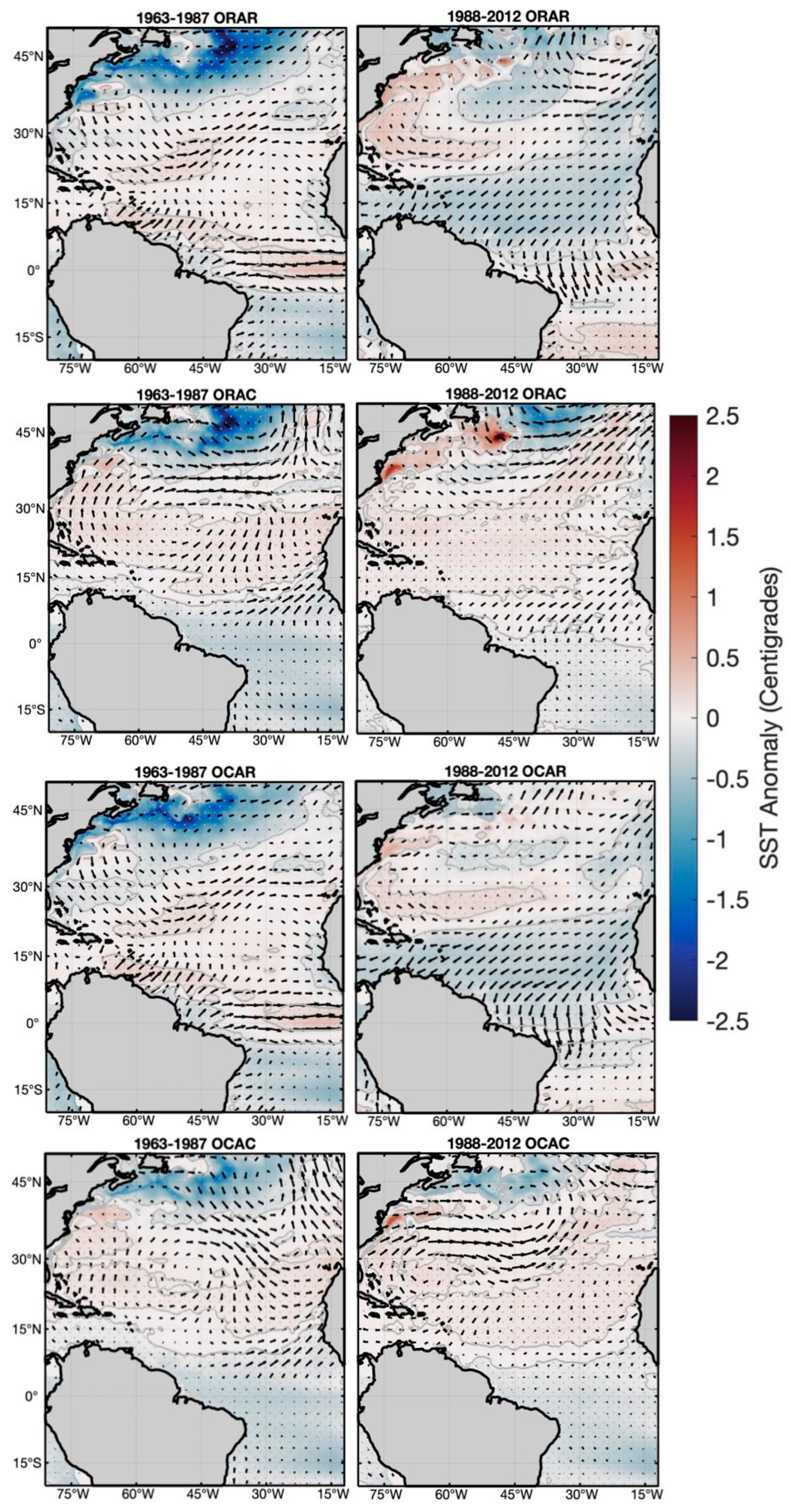
Given the likely significance of the large-scale ocean and atmospheric circulation to the noted change in GS paths, we investigated the modification in wind and SST between the two periods. The composite mean of wind and SST anomalies during times of existing retroflections for the four ensemble experiments are shown for both periods in Figure B1.
Figure B1.
Composite mean of wind and SST anomalies for each ensemble experiment. The anomalies were computed by removing the climatological 50-year averaged monthly mean from the monthly mean of each year. The monthly anomalies were then averaged for when retroflections were taking place.
Figure B1.
Composite mean of wind and SST anomalies for each ensemble experiment. The anomalies were computed by removing the climatological 50-year averaged monthly mean from the monthly mean of each year. The monthly anomalies were then averaged for when retroflections were taking place.
References
- Hogg, N.G. On the transport of the Gulf Stream between Cape Hatteras and the Grand Banks. Deep Sea Research Part A. Oceanographic Research Papers 1992, 39, 1231–1246. [Google Scholar] [CrossRef]
- Kohyama, T.; Yamagami, Y.; Miura, H.; Kido, S.; Tatebe, H.; Watanabe, M. The Gulf Stream and Kuroshio Current are synchronized. Science 374 2021, 341–346. [Google Scholar] [CrossRef] [PubMed]
- Todd, R.E.; Ren, A.S. Warming and lateral shift of the Gulf Stream from in situ observations since 2001. Nature Climate Change 2023, 13, 1348–1352. [Google Scholar] [CrossRef]
- Nye, J.A.; Joyce, T.M.; Kwon, Y.O.; Link, J.S. Silver hake tracks changes in Northwest Atlantic circulation. Nature communications 2011, 2, 412. [Google Scholar] [CrossRef]
- Andres, M. On the recent destabilization of the Gulf Stream path downstream of Cape Hatteras. Geophysical Research Letters 2016, 43, 9836–9842. [Google Scholar] [CrossRef]
- Sánchez-Román, A.; Gues, F.; Bourdalle-Badie, R.; Pujol, M.I.; Pascual, A.; Drévillon, M. Changes in the Gulf Stream path over the last 3 decades. State of the Planet 2024, 4, 1–11. [Google Scholar] [CrossRef]
- Dong, S.; Baringer, M.O.; Goni, G.J. Slow down of the Gulf Stream during 1993–2016. Scientific Reports 2019, 9, 6672. [Google Scholar] [CrossRef]
- Zhang, W.Z.; Chai, F.; Xue, H.; Oey, L.Y. Remote sensing linear trends of the Gulf Stream from 1993 to 2016. Ocean Dynamics 2020, 70, 701–712. [Google Scholar] [CrossRef]
- Silver, A.; Gangopadhyay, A.; Gawarkiewicz, G.; Silva, E.N.S.; Clark, J. Interannual and seasonal asymmetries in Gulf Stream Ring Formations from 1980 to 2019. Scientific Reports 2021, 11, 2207. [Google Scholar] [CrossRef]
- Perez, E.; Andres, M.; Gawarkiewicz, G. Is the regime shift in Gulf Stream warm core rings detected by satellite altimetry? An inter-comparison of eddy identification and tracking products. Journal of Geophysical Research: Oceans 2024, 129, e2023JC020761. [Google Scholar] [CrossRef]
- Pérez-Hernández, M.D.; Joyce, T.M. Two modes of Gulf Stream variability revealed in the last two decades of satellite altimeter data. Journal of Physical Oceanography 2014, 44, 149–163. [Google Scholar] [CrossRef]
- Gangopadhyay, A.; Cornillon, P.; Watts, D.R. A test of the Parsons–Veronis hypothesis on the separation of the Gulf Stream. Journal of Physical Oceanography 1992, 22, 1286–1301. [Google Scholar] [CrossRef]
- Lee, T.; Cornillon, P. Temporal variation of meandering intensity and domain-wide lateral oscillations of the Gulf Stream. Journal of Geophysical Research: Oceans 1995, 100, 13603–13613. [Google Scholar] [CrossRef]
- Taylor, A.H.; Jordan, M.B.; Stephens, J.A. Gulf Stream shifts following ENSO events. Nature 1998, 393, 638–638. [Google Scholar] [CrossRef]
- Joyce, T.M.; Zhang, R. On the path of the Gulf Stream and the Atlantic meridional overturning circulation. Journal of Climate 2010, 23, 3146–3154. [Google Scholar] [CrossRef]
- Taylor, A.H.; Stephens, J.A. The North Atlantic oscillation and the latitude of the Gulf Stream. Tellus A: Dynamic Meteorology and Oceanography 1998, 50, 134–142. [Google Scholar] [CrossRef]
- Gangopadhyay, A.; Chaudhuri, A.H.; Taylor, A.H. On the nature of temporal variability of the Gulf Stream path from 75° to 55°W. Earth Interactions 2016, 20, 1–17. [Google Scholar] [CrossRef]
- Kwon, Y.O.; Joyce, T.M. Northern Hemisphere winter atmospheric transient eddy heat fluxes and the Gulf Stream and Kuroshio–Oyashio Extension variability. Journal of Climate 2013, 26, 9839–9859. [Google Scholar] [CrossRef]
- Joyce, T.M.; Kwon, Y.O.; Seo, H.; Ummenhofer, C.C. Meridional Gulf Stream shifts can influence wintertime variability in the North Atlantic storm track and Greenland blocking. Geophysical Research Letters 2019, 46, 1702–1708. [Google Scholar] [CrossRef]
- Sampe, T.; Nakamura, H.; Goto, A.; Ohfuchi, W. Significance of a midlatitude SST frontal zone in the formation of a storm track and an eddy-driven westerly jet. Journal of Climate 2010, 23, 1793–1814. [Google Scholar] [CrossRef]
- Hotta, D.; Nakamura, H. On the significance of the sensible heat supply from the ocean in the maintenance of the mean baroclinicity along storm tracks. Journal of Climate 2011, 24, 3377–3401. [Google Scholar] [CrossRef]
- Nakamura, H.; Sampe, T.; Tanimoto, Y.; Shimpo, A. Observed associations among storm tracks, jet streams and midlatitude oceanic fronts. Earth’s Climate: The Ocean–Atmosphere Interaction, Geophys. Monogr 2004, 147, 329–345. [Google Scholar] [CrossRef]
- Parfitt, R.; Czaja, A.; Minobe, S.; Kuwano-Yoshida, A. The atmospheric frontal response to SST perturbations in the Gulf Stream region. Geophysical Research Letters 2016, 43, 2299–2306. [Google Scholar] [CrossRef]
- Parfitt, R.; Czaja, A.; Kwon, Y.O. The impact of SST resolution change in the ERA-Interim reanalysis on wintertime Gulf Stream frontal air-sea interaction. Geophysical Research Letters 2017, 44, 3246–3254. [Google Scholar] [CrossRef]
- Soster, F.; Parfitt, R. On objective identification of atmospheric fronts and frontal precipitation in reanalysis datasets. Journal of Climate 2022, 35, 4513–4534. [Google Scholar] [CrossRef]
- Zuo, H.; Balmaseda, M.A.; Mogensen, K.; Tietsche, S. OCEAN5: the ECMWF Ocean Reanalysis System and its Real-Time analysis component. ECMWF Technical Memorandum 2018, 823. [Google Scholar] [CrossRef]
- Zuo, H.; Balmaseda, M.A.; Mogensen, K. The new eddy-permitting ORAP5 ocean reanalysis: description, evaluation and uncertainties in climate signals. Climate Dynamics 2017, 49, 791–811. [Google Scholar] [CrossRef]
- Marshall, J.; Adcroft, A.; Hill, C.; Perelman, L.; Heisey, C. A finite volume, incompressible Navier-Stokes model for studies of the ocean on parallel computers. Journal of Geophysical Research: Oceans 1997, 102, 5753–5766. [Google Scholar] [CrossRef]
- Dewar, W.K.; Parfitt, R.; Wienders, N. Routine reversal of the AMOC in an ocean model ensemble. Geophysical Research Letters 2022, 49, e2022GL100117. [Google Scholar] [CrossRef]
- Jamet, Q.; Dewar, W.K.; Wienders, N.; Deremble, B. Spatiotemporal patterns of chaos in the Atlantic overturning circulation. Geophysical Research Letters 2019, 46, 7509–7517. [Google Scholar] [CrossRef]
- Jamet, Q.; Dewar, W.K.; Wienders, N.; Deremble, B.; Close, S.; Penduff, T. Locally and remotely forced subtropical AMOC variability: A matter of time scales. Journal of Climate 2020, 33, 5155–5172. [Google Scholar] [CrossRef]
- Uchida, T.; Jamet, Q.; Dewar, W.K.; Le Sommer, J.; Penduff, T.; Balwada, D. Diagnosing the thickness-weighted averaged eddy-mean flow interaction from an eddying North Atlantic ensemble: The Eliassen-Palm flux. Journal of Advances in Modeling Earth Systems 2022, 14, e2021MS002866. [Google Scholar] [CrossRef]
- Uchida, T.; Jamet, Q.; Dewar, W.K.; Deremble, B.; Poje, A.C.; Sun, L. Imprint of chaos on the ocean energy cycle from an eddying North Atlantic ensemble. Journal of Physical Oceanography 2024, 54, 679–696. [Google Scholar] [CrossRef]
- Uchida, T.; Jamet, Q.; Poje, A.C.; Wienders, N.; Dewar, W.K. Wavelet-based wavenumber spectral estimate of eddy kinetic energy: Application to the North Atlantic. Ocean Modelling 2024, 102392. [Google Scholar] [CrossRef]
- Lillibridge, I.I.I.; JL; Mariano, A. J. A statistical analysis of Gulf Stream variability from 18+ years of altimetry data. Deep Sea Research Part II: Topical Studies in Oceanography 2013, 85, 127–146. [Google Scholar] [CrossRef]
- Rossby, T.; Flagg, C.N.; Donohue, K.; Sanchez-Franks, A.; Lillibridge, J. On the long-term stability of Gulf Stream transport based on 20 years of direct measurements. Geophysical Research Letters 2014, 41, 114–120. [Google Scholar] [CrossRef]
- Sheremet, V.A. Inertial gyre driven by a zonal jet emerging from the western boundary. Journal of Physical Oceanography 2002, 32, 2361–2378. [Google Scholar] [CrossRef]
- Worthington, L.V. On the north Atlantic circulation. John Hopkins Oceanographic Studies 1976, 6, 110. [Google Scholar]
- Schmitz Jr, W.J. On the eddy field in the Agulhas Retroflection, with some global considerations. Journal of Geophysical Research: Oceans 1996, 101, 16259–16271. [Google Scholar] [CrossRef]
- Hansen, D.V. Gulf stream meanders between Cape Hatteras and the Grand Banks. Deep Sea Research and Oceanographic Abstracts 1970, 17, 495–511. [Google Scholar] [CrossRef]
- Berger, V.W.; Zhou, Y. (2014). Kolmogorov–smirnov test: Overview. Wiley statsref: Statistics reference online. [CrossRef]
- Chakravorty, S.; Czaja, A.; Parfitt, R.; Dewar, W.K. (2024). Tropospheric response to Gulf Stream intrinsic variability: a model ensemble approach. Geophysical Research Letters. [CrossRef]
- Seo, H.; O’Neill, L.W.; Bourassa, M.A.; Czaja, A.; Drushka, K.; Edson, J.B.; Wang, Q. Ocean mesoscale and frontal-scale ocean–atmosphere interactions and influence on large-scale climate: A review. Journal of climate 2023, 36, 1981–2013. [Google Scholar] [CrossRef]
- Megann, A.; Blaker, A.; Josey, S.; New, A.; Sinha, B. Mechanisms for late 20th and early 21st century decadal AMOC variability. Journal of Geophysical Research: Oceans 2021, 126, e2021JC017865. [Google Scholar] [CrossRef]
- Aldama-Campino, A.; Döös, K. Mediterranean overflow water in the North Atlantic and its multidecadal variability. Tellus A: Dynamic Meteorology and Oceanography 2020, 72, 1–10. [Google Scholar] [CrossRef]
Figure 1.
Gulf Stream path given by the −11 cm SSH isoline in ORAS5 for November of 2012 is shown in white curve (a). The horizontal current speed is plotted in the background. The green portion of the trajectory about 57°W and 41°N is what we define in this study as a retroflection. Mean Gulf Stream path detected from the ORAS5 product and the four ensemble experiments (b). The thick curves represent the mean over the 50 years of record (1963-2012) of the −11 cm SSH isoline for the reanalysis and 25 cm for the ensemble mean. The intervals in shading represent one standard deviation.
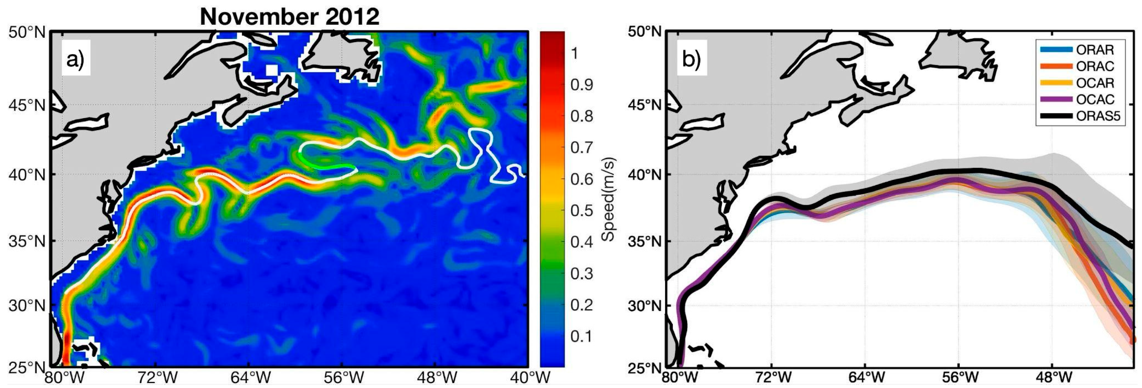
Figure 2.
GS path length computed for the four ensemble experiments (a-d) and the ORAS5 product (f). The blue time series represents the path length computed in the region defined zonally between 75°W-50°W and the orange line for the entire zonal extent of the SSH contour. We remind the reader that we are analyzing the ensemble-mean paths for the ensembles while the single (and ‘true’) realization from ORAS5. .
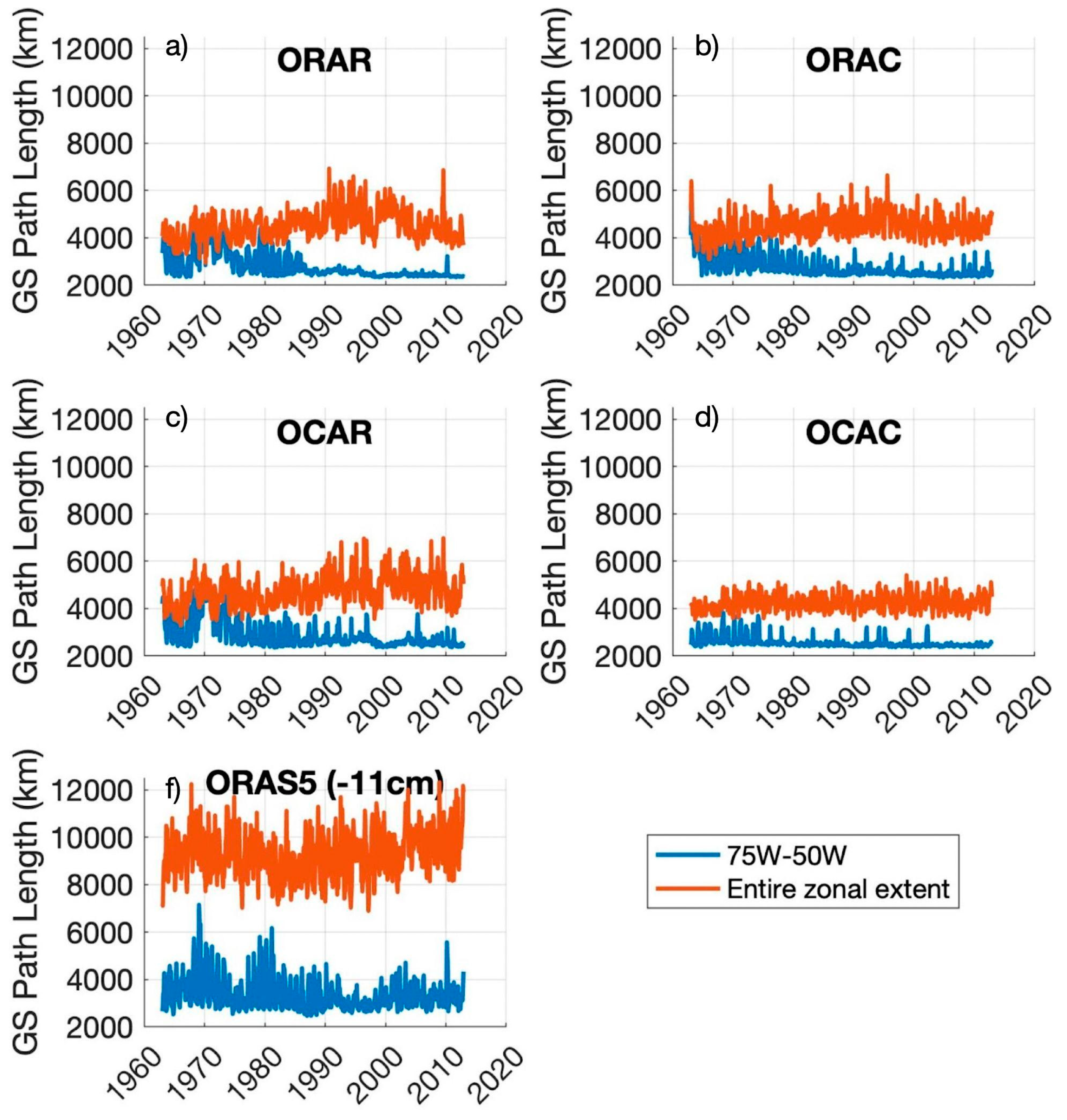
Figure 3.
Distribution of the longitude where the Gulf Stream path retroflection closest to its point of separation occurs in the ORAS5 data for the first 25 years (a) and latter 25 years (b). The histograms are displayed in blue and in black curve the associated probability density function (PDF) for the −11 cm SSH contour. The number of retroflections, the mean, variance, skewness and kurtosis of each PDF are shown. The same figure but for the other SSH contours analyzed is presented in Appendix A. .
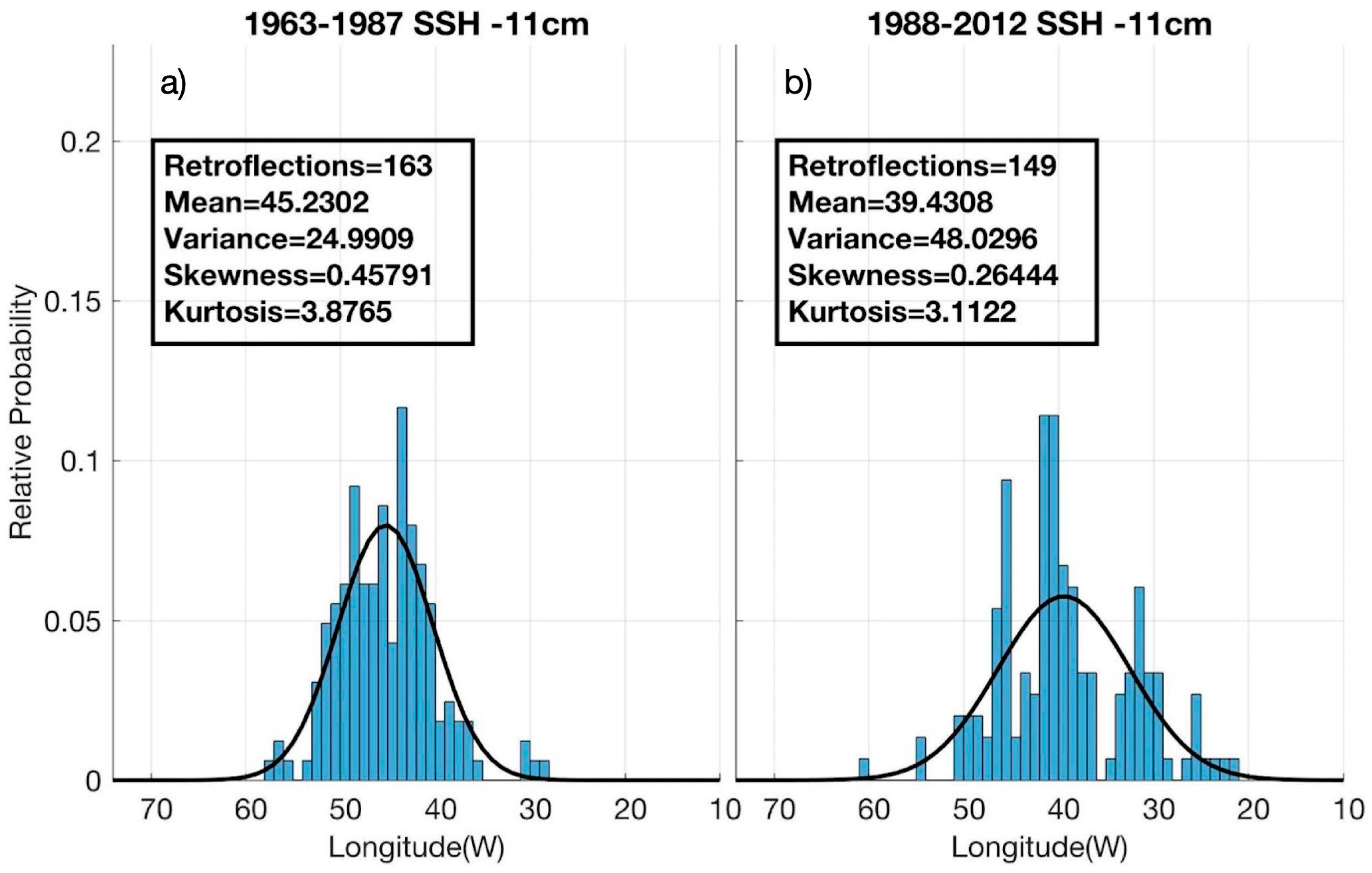
Figure 4.
Same as Figure 3 but for the ensemble-mean GS path from all four ensemble experiments (ORAR, ORAC, OCAR and OCAC).
Figure 4.
Same as Figure 3 but for the ensemble-mean GS path from all four ensemble experiments (ORAR, ORAC, OCAR and OCAC).
Disclaimer/Publisher’s Note: The statements, opinions and data contained in all publications are solely those of the individual author(s) and contributor(s) and not of MDPI and/or the editor(s). MDPI and/or the editor(s) disclaim responsibility for any injury to people or property resulting from any ideas, methods, instructions or products referred to in the content. |
© 2024 by the authors. Licensee MDPI, Basel, Switzerland. This article is an open access article distributed under the terms and conditions of the Creative Commons Attribution (CC BY) license (http://creativecommons.org/licenses/by/4.0/).
Copyright: This open access article is published under a Creative Commons CC BY 4.0 license, which permit the free download, distribution, and reuse, provided that the author and preprint are cited in any reuse.


