
Submitted:
14 November 2024
Posted:
18 November 2024
You are already at the latest version
Abstract
Accurate localization is crucial for numerous applications. While several methods exist for out-door localization, typically relying on GPS signals, these approaches become unreliable in indoor environments due to weak GPS signal or GPS outage. Many researchers have attempted to ad-dress this limitation, primarily focusing on real-time solutions. However, for applications that do not require real-time localization, these methods remain suboptimal. This paper presents a novel Transformer-based bidirectional encoder approach to address indoor localization challenges in postprocessing. Our method predicts velocity during periods of weak or lost GPS signal and calculates position through bidirectional velocity integration. Additionally, it incorporates posi-tion interpolation to ensure smooth transitions between active GPS and GPS outage phases. Applied to a dataset tracking horse positions—which features velocities up to 10 times those of pedestrians and higher acceleration—our approach achieved an average trajectory error below 3 meters, while maintaining stable relative distance errors regardless of GPS outages duration.
Keywords:
indoor localization reconstruction
; transformer
; bidirectional encoder
; deep learning
; time series
1. Introduction
A widely used approach for 3D localization is the Inertial Measurement Unit (IMU) [1], which typically includes accelerometers, gyroscopes, and occasionally magnetometers. IMUs provide 3D acceleration and orientation data. However, due to inherent noise, IMU-based localization (which requires double integration of acceleration) is prone to significant temporal drift [2], making reliable positioning feasible for only brief periods. To address this, IMU data are often combined with Global Positioning System (GPS) data through a Kalman Filter (KF) [3].
In outdoor environments, combining IMU and GPS data with a KF enables accurate localization. However, in indoor settings, this approach is limited by GPS signal issues, such as weak signal or signal loss. Since the sensor’s localization depends heavily on GPS data, its accuracy declines sharply indoors.
Deep learning-based methods have been developed to provide real-time localization during GPS outages by leveraging information from past data. Although these methods can also offer localization for applications that do not require real-time processing, they have a limitation: they cannot utilize future data. Thus, these approaches lead to suboptimal localization when both past and future data can be used.
In this paper, we present a novel deep learning approach using a Transformer-based bidirectional encoder to reconstruct indoor localization during postprocessing. This approach employs raw IMU and GPS data, along with the KF output, to predict velocity. Position is then obtained by bidirectional integration of this velocity data. We also incorporate position interpolation to ensure smooth transitions between recorded and predicted positions during GPS outages.
The proposed approach is tested using the Alogo Move Pro sensor, a device specifically designed for equestrian applications. This device uses an Inertial Navigation System (INS) that combines IMU and GPS data through a KF, enabling 3D localization of a horse during training and competition. Based on this localization, the device generates various metrics such as stride analysis, power, and maximum jump height. Riders typically review session data after training or competition, allowing for postprocessing and enabling to leverage information from both past and future data when applying localization reconstruction.
The sensor’s outdoor accuracy has been validated [4]. However, in indoor environments, the sensor experiences GPS outages, compromising the precision required for effective analysis of horse behaviors. GPS outages in the sensor occur in three main cases: at the start, during, or at the end of a session. Additionally, GPS outages duration can be categorized into short outages (10 to 20 seconds) and medium outages (30 seconds to 2 minutes).
2. Related Works
Many researchers have explored ways to reduce noise in IMU data by investigating alternative fusion methods that do not rely on GPS data. Several factors may drive the choice to use only IMU data, including the cost of adding a GPS receiver and the impracticality of GPS in certain contexts, such as indoor localization within buildings. Sun et al. [5] proposed a two-stage pipeline to address this challenge: first predicting device orientation and then estimating position based on IMU data from a smartphone. Their approach utilized a Long Short-Term Memory (LSTM) network in the first stage and a bidirectional LSTM network in the second. Chen et al. [6] introduced a method that segments IMU data into windows, applying an LSTM network to learn the relationship between raw acceleration data and the polar delta vector, from which localization is derived. Brossard et al. [7] took a different approach, presenting a Convolutional Neural Network (CNN) to correct gyroscope noise in raw IMU signals.
In another study [8], the authors proposed an extended KF based on a 1D version of ResNet18 to fuse IMU data for localization estimation. A more lightweight adaptation of this approach, compatible with standard smartphones, was developed in [9]. Similarly, Wang et al. [10] proposed a ResNet18-inspired network for fusing IMU data. Cioffi et al. [11], focusing on drones, adopted a Temporal Convolutional Network (TCN), citing studies showing that TCNs perform comparably to Recurrent Neural Networks (RNNs) for temporal sequences, with the added advantages of easier training and deployment on robotic platforms. Rao et al. [12] introduced a contextual transformer network with a spatial encoder and a temporal decoder to fuse IMU data for velocity prediction, which allowed localization via velocity integration. Wang et al. [13] achieved high localization accuracy from IMU data using a network with convolution blocks, a bidirectional LSTM, and a Multi-Layer Perceptron (MLP), incorporating an attention mechanism.
Other studies have aimed to improve the fusion of IMU and GPS data, which is traditionally managed through a KF. Hosseinyalamdary [14] presented a deep KF using an LSTM to fuse IMU and GPS data, achieving better localization than the conventional KF. Wu et al. [15] replaced the KF with a TCN for position and velocity prediction, adopting a multitask strategy to reduce prediction errors. Lastly, Kang et al. [16] developed a model combining a CNN with a Gated Recurrent Unit (GRU) to predict pedestrian velocity.
This literature review indicates that extensive efforts have been made to either predict localization from IMU data alone or enhance GPS and IMU data fusion. However, the problem of GPS signal loss has received limited attention, with most studies addressing GPS outages in real-time applications. As a result, these real-time methods cannot leverage the benefits of a postprocessing bidirectional perspective. While such methods may work for applications not requiring real-time localization, they yield suboptimal results. To address this gap, we propose a deep learning approach for localization reconstruction in postprocessing, utilizing both past and future data to improve localization accuracy.
3. Materials
3.1. Data
To develop our deep learning approach, we collected data from the Alogo Move Pro device during outdoor sessions. The data capture a variety of contexts, including training sessions, equestrian trails, and competition courses. In total, 53 sessions were recorded, amounting to 29 hours and 4 minutes of data. The shortest session lasted 27 seconds, while the longest extended to 49 minutes and 57 seconds. The average session duration was 32 minutes and 54 seconds, with a standard deviation of 12 minutes and 48 seconds. The sessions were divided into three datasets: training (64%), validation (18%), and testing (18%).
Each session consists of 100 timestamps per second, and for each timestamp, the device provides the following data:
- AXIMU, AYIMU, AZIMU: Acceleration measured by the IMU
- RAIMU, RBIMU, RCIMU: Rate of rotation measured by the IMU
- MXIMU, MYIMU, MZIMU: Magnetic field measured by the IMU
- PXGPS, PYGPS, PZGPS: Position measured by the GPS
- VXGPS, VYGPS, VZGPS: Velocity measured by the GPS
- EGPS: Position accuracy estimation provided by the GPS (PDOP)
- PXFUSION, PYFUSION, PZFUSION: Position computed by the sensor fusion algorithm
- VXFUSION, VYFUSION, VZFUSION: Velocity computed by the sensor fusion algorithm
- OAFUSION, OBFUSION, OCFUSION: Orientation computed by the sensor fusion algorithm
- EFUSION: Position accuracy estimation provided by the sensor algorithm
GPS data are refreshed at a frequency of 5 Hz, while IMU and sensor fusion algorithm data are refreshed at 100 Hz. Table A1 presents various statistical details about these features across the entire dataset.
The PFUSION, VFUSION and OFUSION values are computed by the sensor fusion algorithm using IMU data (AIMU, RIMU, and MIMU) and GPS data (PGPS and VGPS). During GPS outages or periods of weak GPS signal, the accuracy of PGPS and VGPS declines, which affects PFUSION, VFUSION and OFUSION due to error propagation. In this study, our primary goal is to accurately reconstruct PFUSION during these GPS outage phases.
3.2. Testing Subdatasets
As outlined in the introduction, there are three primary cases of GPS outages: at the beginning of the session, during the session, and at the end of the session. Additionally, GPS outages can be categorized by duration into two types: short outages (10 to 20 seconds) and medium outages (30 seconds to 2 minutes). To simulate these scenarios, we created three masking schemas to generate testing subdatasets from the original testing dataset:
- Schema 1: The beginning of the session is masked
- Schema 2: A section within the session is masked, while the beginning and end of the session remain unmasked (at least 2 seconds are left unmasked at both the start and end).
- Schema 3: The end of the session is masked
The lengths of the masked sections (denoted as Lmask) and the positions of the mask within the session (denoted as Pmask) for schema 2 were randomly sampled from a uniform distribution. To expand the testing subdatasets, each session was duplicated multiple times, with each duplicate receiving a different mask sampled from the same distribution (see Figure 1).
For each schema, we created two subdatasets: one simulating short GPS outages (10 s < Lmask < 20 s) and another simulating medium GPS outages (30 s < Lmask < 120 s). The masking process was implemented by setting the following features to null values, preventing the model from accessing this information during localization reconstruction:
- GPS features: PXGPS, PYGPS, PZGPS, VXGPS, VYGPS, VZGPS, EGPS
- Sensor fusion algorithm output features: PXFUSION, PYFUSION, PZFUSION, VXFUSION, VYFUSION, VZFUSION, OAFUSION, OBFUSION, OCFUSION, EFUSION
3.3. Preprocessing
Since the sensor is used across multiple countries, the GPS and sensor fusion algorithm positions (PGPS and PFUSION) vary significantly in range. To address this, we converted all positions to relative positions. For the training and validation datasets, as well as the testing subdatasets based on schemas 2 and 3, relative positions were calculated using each session’s first position. For testing subdatasets based on schema 1, relative positions were calculated based on the first position after the masked section.
Next, we applied normalization [17] to scale the features to the range [0, 1]. Additionally, we created a separate velocity vector (a duplicate of VXFUSION, VYFUSION, VZFUSION) to serve as the target for training our neural network, with normalization applied in the range [-1, 1].
4. Approach
4.1. Flow
To reconstruct the localization of a horse during a GPS outage, we propose a six-step process, illustrated in Figure 2.
Extracting the GPS outage section: The GPS outage section is isolated from the session to create a window of size Lseq, containing all sensor features (listed in Section 3.1. Data) at a frequency of 100 Hz. For short GPS outages (up to 20 seconds), we define Lseq = 2400 (24 seconds). For medium GPS outages (up to 120 seconds), Lseq = 12400 (124 seconds). This ensures that the window includes at least 4 seconds of data not recorded during a GPS outage. For outages at the beginning or end of a session, the valid GPS data will be positioned at one extremity of the window. For outages occurring mid-session, valid data will be available at both sides, allowing the network access to past and/or future data to inform its predictions.
Masking GPS outage timestamps: Timestamps within the GPS outage are selected, and features dependent on GPS are masked to signify the outage to the neural network. Masking is applied by replacing values with -1.
Neural network processing: The processed window is fed into the neural network, which outputs velocity predictions across three axes. Tests indicated that directly predicting positions resulted in poor performance. As illustrated in Figure 3, velocity distributions are consistently centered around 0 across sessions, while position distributions are highly variable due to differences in session types and distances covered. Therefore, predicting velocities—constrained within a typical range—is more stable than predicting positions, which may vary extensively.
Integrating velocities: Positions are derived by integrating the predicted velocities. For outages at the beginning or end of a session, positions are computed unidirectionally. For mid-session outages, a bidirectional integration (forward and backward) is performed, and the results are averaged to distribute position errors more evenly across the GPS outage section.
Applying interpolation (only for GPS outage in the middle of a session): Because bidirectional integration can create discontinuities with the rest of the session, an interpolation step is applied at the boundaries of the GPS outage. To achieve smooth junctions, we calculate the duration of data to be interpolated at each extremity of the GPS outage section, denoted as tinterp (illustrated in Figure 4). Two quadratic interpolation functions are fitted—one at each boundary. The first function is fitted using data from the 20 ms before the outage and the 20 ms after tinterp seconds at the beginning of the outage. The second function uses data from the 20 ms preceding tinterp seconds at the end of the outage and the 20 ms following the outage. These functions are then applied to the first and last tinterp seconds of the predicted positions. The process is illustrated in Figure 5.
Merging results: The final integrated (and interpolated, if applied) positions are merged back into the session.
As we might note, our approach is based on a Transformer network, which poses training challenges due to high computational demands and GPU memory requirements. Given the complexity of Transformers concerning input sequence length, we also propose a lighter variant of our approach that processes data at a frequency of 10 Hz instead of 100 Hz. In this version, the network outputs the average velocities over 10 timestamps rather than per timestamp.
4.2. Network Architecture
Our proposed network architecture is inspired by the BERT model [18]. The network consists of multiple Transformer encoder layers stacked sequentially, followed by a feed-forward layer. To improve precision, the model uses a learnable positional encoding that is updated during training. The architecture is shown in Figure 2. We define dmodel as the dimension of the embedding, Nhead the number of head in the multi head attentions, dhidden the size of the inner layer of the feed forwards and Nencoder the number of encoder layers.
The network takes as input a sequence where is the dimension of the input sequence and Lseq is the length of the sequence as defined in section 4.1. Flow. Initially, the input sequence is projected into the embedding space :
where and Then, the learnable positional encoding is added to the projected input:
After the input projection and positional encoding, the sequence is processed through Nencoder encoder layers. Each encoder layer has an identical structure but unique weights and biases. Each layer consists of a residual multi-head attention mechanism followed by a residual feed-forward network.
The residual multi-head attention mechanism, as described by Vaswani et al. in the original Transformer paper [19], is defined as follows:
where , , , and The residual feed-forward network, as described by Vaswani et al. in [19], is given by:
where , , , and After processing through the Nencoder encoder layers, the sequence passes through a final feed-forward network that projects it into , representing the velocities along the x, y, and z axes for the entire sequence:
where , , , and .
4.3. Network Training
The network was trained for up to 500 epochs, with early stopping applied if no improvement was observed for 20 consecutive epochs [20].
To train and validate the network, sequences of length Lseq were extracted from the training and validation sessions. For small GPS outage sections (10 to 20 seconds), Lseq was set to 2400 (or 240 for the lighter network version). For medium GPS outage sections (30 seconds to 2 minutes), Lseq was set to 12400 (or 1240 for the lighter version). To extract sequences, we sampled 1/5000th of the timestamps in training sessions as sequence starting points, while 1/1000th of timestamps were sampled in validation sessions. During training, the sampled timestamps were rotated through the dataset every 20 epochs, while validation timestamps remained fixed. This process is illustrated in Figure 6.
Each sequence was assigned a mask of size Lmask, where Lmask was sampled from a uniform distribution. For small GPS outage training, (for the lighter version: ), and for medium GPS outage training, (for the lighter version: ). We explored several masking strategies (where Pmask is the first index of the mask on the sequence):
- Strategy 1: Mask applied at the start of the sequence,
- Strategy 2: Mask applied in the center of the sequence,
- Strategy 3: Mask applied at the end of the sequence,
- Strategy 4: Mask applied at a random position,
Strategies 1, 2, and 3 were tailored for schemas 1, 2, and 3, respectively, while strategy 4 was intended for use across all schemas. During training, the mask length (and position for strategy 4) was regenerated at each epoch, while validation masks remained constant. Masking was performed by setting GPS and sensor fusion features to -1:
- GPS features: PXGPS, PYGPS, PZGPS, VXGPS, VYGPS, VZGPS, EGPS
- Sensor fusion algorithm output features: PXFUSION, PYFUSION, PZFUSION, VXFUSION, VYFUSION, VZFUSION, OAFUSION, OBFUSION, OCFUSION, EFUSION
The network was trained to reconstruct the velocity using the Adam optimizer with weight decay [21]. To emphasize minimizing large prediction errors, we selected the Mean Square Error (MSE) loss function. Additionally, we hypothesized that encouraging the network to predict velocity in both the masked and unmasked sections could improve results by promoting continuity. Therefore, we constructed a dual-objective function that considers both masked and unmasked sections:
where is the masked part of the sequence and is a hyperparameter, and are respectively the ground truth velocity and the predicted velocity of the ith timestamp of the sequence.
4.4. Hyperparameter Tuning
4.5. Evaluation
To evaluate our approach, we defined three metrics:
- The Absolute Trajectory Error (ATE): Measures the discrepancy between the ground truth and the predicted trajectories. This metric is sensitive to outliers. Therefore, it is common that this metric increases with prediction duration and length.
- The Relative Trajectory Error (RTE): Quantifies the relative error in the distance between the ground truth and predicted start/end points.
- The Relative Distance Error (RDE): Calculates the relative error between the total predicted and ground truth distances.
- is the ground truth position in 3D at instant t:
- is the predicted position in 3D at instant t:
- is the Euclidean norm between and
5. Results
Our approach achieves an ATE of approximately 3 meters for small GPS outages across the entire testing dataset. For medium GPS outages, the ATE is around 12 meters. This means that, on average, the predicted positions for small GPS outages are within 3 meters of the actual position of the horse, and for medium GPS outages, within 12 meters. In comparison, state-of-the-art methods on pedestrian datasets, which feature shorter distances, lower velocities (up to 10 times slower), and reduced acceleration, report ATE values mostly between 4 and 9 meters for GPS outages of several seconds to minutes [5,9,10,12].
For the RTE, our approach yields values ranging from 0.2 to 0.7. This implies that the ratio of the distance between the predicted end point and the predicted start point relative to the distance between the actual end point and start point falls between 0.2 and 0.7. In contrast, state-of-the-art methods report RTE values ranging from 0.9 to 6 for one-minute GPS outages in pedestrian contexts [5,9,10,12].
In terms of RDE, our approach also performs well, averaging 0.3 regardless of GPS outage duration, highlighting stable performance across various outage lengths. A summary of these results is provided in Table 2 and Table 3.
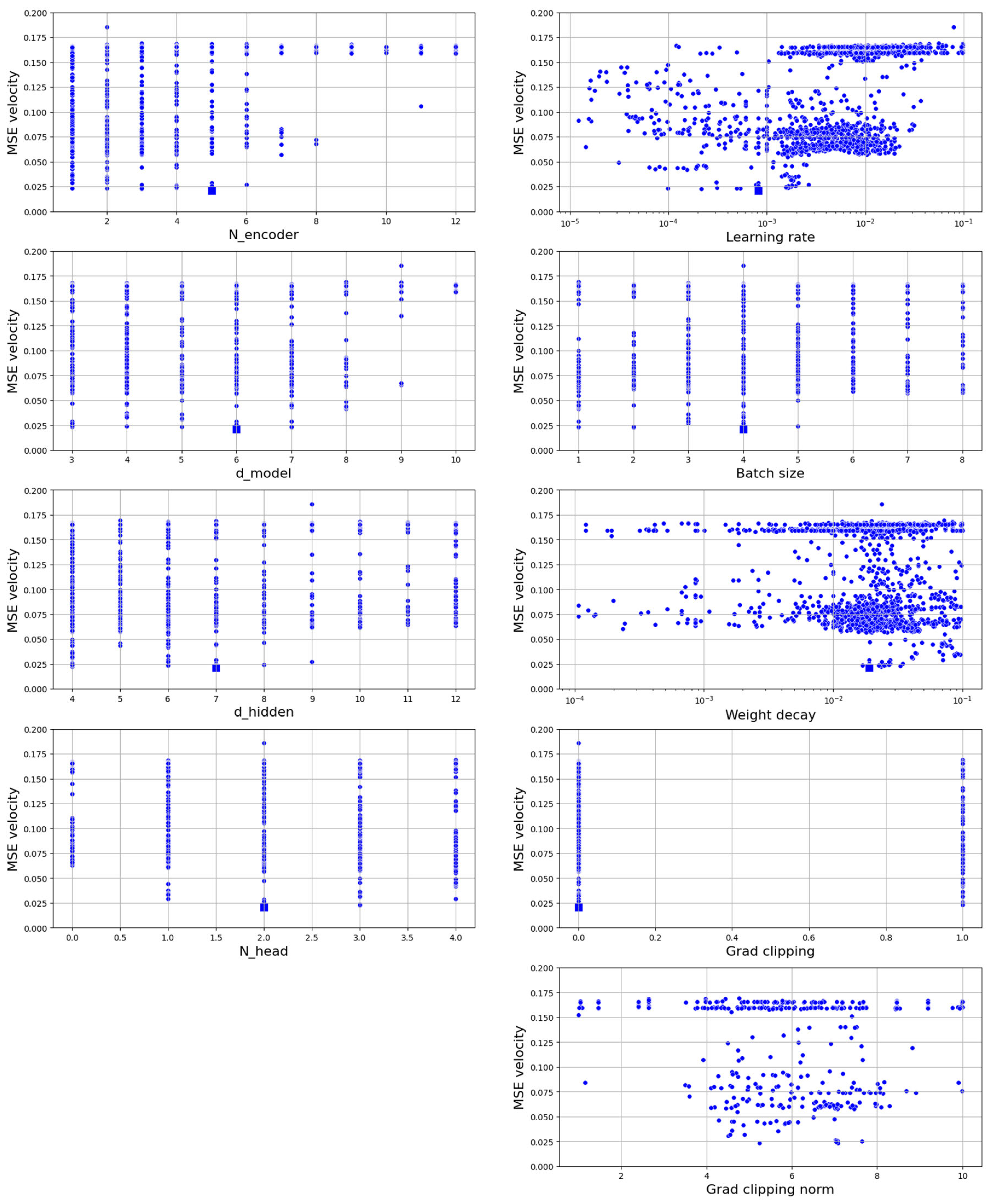
Regarding the hyperparameters space, we determined an optimal subspace and the best hyperparameters set, available in Table 4. A more detailed illustration of the results of the hyperparameters search is available in Figure B1.
Another crucial aspect for real-world applications is quantifying the processing time of the deep neural network, which represents the majority of our approach’s computation time, and assessing memory consumption.
With the best-performing hyperparameter configuration, the network can make an inference on a CPU in 160 ms for small GPS outages and 5.01 s for medium GPS outages. For applications requiring more rapid responses, the lighter network version completes predictions on a CPU in 4.14 ms for small GPS outages and 49 ms for medium GPS outages. On a GPU, prediction times decrease significantly: 3.05 ms (1.76 ms for the lighter version) for small GPS outages and 57.8 ms (1.80 ms for the lighter version) for medium GPS outages. GPU memory consumption is relatively low, with most modern GPUs having ample memory for this task.
Using the best hyperparameter configuration, training on a CPU is impractically slow. However, on a GPU, even a basic model with a few GB of RAM is sufficient. Table 5 provides detailed specifications of the network with the optimal hyperparameters.
For applications requiring hyperparameter searches in the explored space, we recommend a high-performance GPU, as larger networks may demand up to several dozen GB of RAM. Additional information on processing time and memory usage for various network sizes is available in Appendix C.
As shown in Figure 7, our approach accurately predicts the velocity trends and amplitudes, while avoiding adherence to velocity noise, demonstrating the network’s robustness. For position predictions, there is a close alignment with the ground truth signal. Although minor deviations exist at certain points, they appear to be well-balanced by the positive and negative errors within the velocity signals, with occasional accumulations being compensated over time.
From a top-view perspective (illustrated in Figure 8, as seen by riders in the sensor application), the predicted positions align well, and the interpolation step following position integration creates a seamless transition between the GPS outage section and the rest of the session.
6. Discussion
In this research, we compared fixed masking strategies (strategies 1, 2, and 3) with a random masking strategy (strategy 4) to train the network. Each fixed strategy is designed for a specific schema, while the random strategy is applicable across all three schemas. On average, both fixed and random strategies produced nearly identical results in most cases. Depending on the schema, either a fixed or random strategy yielded the best results (see Figure 9). Thus, while training all four strategies achieves highly accurate results, training only the random strategy can achieve good results with a quarter of the computational cost.
Regarding input frequency (100 Hz for the base version, 10 Hz for the lighter version), we observed similar results for both, with better outcomes in some cases at 10 Hz (see Figure 9). This may seem surprising at first, but is logical: a lower frequency reduces precision in velocity predictions (predicting the mean over 100 ms rather than every 10 ms). However, velocity errors are well-distributed (balanced between positive and negative errors) over the 100 ms period, so after integration, they cancel out, preventing drift. The only noticeable errors are short-lived (within 100 ms) and correlate with the duration before positive and negative velocity errors balance out. Additionally, the lighter network’s reduced input sequence length allows for faster training, freeing up resources to explore more hyperparameter sets and increasing the chance of finding an optimal configuration. Moreover, even with a GPU with 25 GB of RAM, some configurations remain untested on the base version due to excessive memory requirements, especially for sequences up to 2 minutes in length.
We computed hyperparameter importance (shown in Figure 10). For model architecture, the number of encoder layers Nencoder and the embedding dimension dmodel were the most impactful hyperparameters. In training configuration, the learning rate was the most influential, followed by batch size and weight decay.
Despite these promising results, several areas of our approach warrant further exploration.
Validation in indoor environments: Our approach, designed to predict velocity during GPS outages, was trained on sequences extracted from outdoor sessions. However, horses can exhibit different behaviors (in stride, jump, velocity, and acceleration) between indoor and outdoor environments. Thus, results based on outdoor data do not guarantee accuracy indoors. To validate our approach for indoor use, data would need to be collected in indoor settings, with performance evaluated on masked sequences from those sessions. If indoor performance proves less accurate, retraining the network with both outdoor and indoor data may be necessary. However, because accurate ground truth cannot be obtained in indoor settings with our sensor due to GPS outages, recording such sessions would require a more sophisticated setup not reliant on GPS and IMU. For example, a combination of UWB and LiDAR could provide reliable ground truth in indoor environments. We did not conduct this experiment due to the high cost of such setups, which can reach hundreds of thousands of euros.
Computational requirements for longer GPS outages: The computational resources required for training and predicting velocity during GPS outages increase exponentially with input sequence length. We introduced a lighter version of our approach, which achieved similar accuracy by reducing the input frequency by a factor of ten. However, even with this adjustment, handling large GPS outages (e.g., 5 to 10 minutes) is challenging and demands substantial computational infrastructure. Preliminary attempts to reduce input frequency further (by a factor of hundred) compromised accuracy. For longer GPS outage duration, future work could explore advanced attention mechanisms that replicate the performance of standard Transformer attention while reducing computational costs.
Validation across different devices and use cases: We validated our approach on a dataset of horse positions recorded using the Alogo Move Pro device. Future work could expand validation to different devices and various types of motion (e.g., pedestrians, cyclists, racing dogs, drone) to assess the generalizability of the approach.
Conclusions
This paper presents a novel Transformer-based approach to reconstruct indoor localization during postprocessing. Our method leverages a neural network to predict velocity, from which position is then obtained through bidirectional integration (or unidirectional when bidirectional is not feasible) to better distribute position errors. A final interpolation step ensures smooth transitions between known and predicted positions.
Experiments demonstrate that our approach achieves an ATE of approximately 3 meters for short GPS outages (10 to 20 seconds) and around 12 meters for medium GPS outages (30 seconds to 2 minutes), which is highly encouraging compared to state-of-the-art results primarily focused on pedestrians rather than horses.
Despite the neural network's computational complexity, predictions can be made on both CPU and GPU without specialized requirements. For applications needing rapid predictions, we also propose a lighter version that achieves accuracy close to the base model while reducing the required sequence length by a factor of ten for the same GPS outage duration. However, training on a CPU remains impractical. Moreover, for hyperparameter exploration, we recommend a high-performance GPU with substantial RAM capacity.
While this research introduces a novel and effective solution that addresses a gap in existing literature, several areas remain for future exploration: evaluating the model on indoor data acquired with a UWB and LiDAR setup, reducing the model’s computational complexity to handle longer GPS outages, and extending validation to other types of motion beyond horses.
Author Contributions
Conceptualization, Kévin Guyard and Jonathan Bertolaccini; Data curation, Kévin Guyard; Formal analysis, Kévin Guyard; Funding acquisition, Stéphane Montavon and Michel Deriaz; Investigation, Kévin Guyard; Methodology, Kévin Guyard; Project administration, Kévin Guyard and Jonathan Bertolaccini; Software, Kévin Guyard; Supervision, Kévin Guyard and Jonathan Bertolaccini; Validation, Kévin Guyard; Visualization, Kévin Guyard; Writing – original draft, Kévin Guyard; Writing – review & editing, Kévin Guyard and Jonathan Bertolaccini.
Funding
This work was carried out as part of the project Alina, supported by Innosuisse.
Institutional Review Board Statement
This study was conducted during regular training of riders with their horses. It complies with the Code of Conduct of the Federation Equestre Internationale (FEI) and the Swiss legislation concerning the codes of ethical behavior in the animal and human domains.
Informed Consent Statement
Informed consent was obtained from all riders involved in the study.
Data Availability Statement
The raw data supporting the conclusions of this article will be made available by the authors on request.
Acknowledgments
The authors thank David Deillon for loaning an Alogo Move Pro sensor used to collect the data for this study.
Appendix A

Table A1.
Statistic of the dataset features (statistics for position features are given after the transformation from absolute to relative position).
Table A1.
Statistic of the dataset features (statistics for position features are given after the transformation from absolute to relative position).
| Mean | Std | Min | Q1 | Median | Q3 | Max | |
|---|---|---|---|---|---|---|---|
| AXIMU | −2.35 × 10⁻¹ | 4.53 × 100 | −1.10 × 10² | −1.95 × 100 | −7.50 × 10⁻² | 1.80 × 100 | 1.03 × 10² |
| AYIMU | 1.32 × 10⁻¹ | 3.32 × 100 | −8.73 × 101 | −1.53 × 100 | 1.55 × 10⁻¹ | 1.81 × 100 | 1.60 × 10² |
| AZIMU | −9.97 × 100 | 6.06 × 100 | −1.10 × 10² | −1.17 × 101 | −9.85 × 100 | −8.12 × 100 | 9.98 × 101 |
| RAIMU | −8.93 × 10⁻² | 2.61 × 101 | −3.27 × 10² | −1.24 × 101 | −4.00 × 10⁻² | 1.23 × 101 | 3.25 × 10² |
| RBIMU | 6.47 × 10⁻¹ | 3.92 × 101 | −3.27 × 10² | −2.54 × 101 | −1.71 × 100 | 2.49 × 101 | 3.27 × 10² |
| RCIMU | −7.51 × 10⁻¹ | 2.74 × 101 | −3.08 × 10² | −1.81 × 101 | −3.90 × 10⁻¹ | 1.68 × 101 | 3.20 × 10² |
| MXIMU | −4.09 × 10⁻¹ | 7.57 × 101 | −2.36 × 10² | −4.99 × 101 | −2.65 × 100 | 4.84 × 101 | 2.04 × 10² |
| MYIMU | 6.04 × 101 | 8.75 × 101 | −2.00 × 10² | −5.74 × 100 | 6.09 × 101 | 1.25 × 10² | 3.02 × 10² |
| MZIMU | −1.78 × 101 | 1.22 × 10² | −2.30 × 10² | −1.49 × 10² | 9.66 × 100 | 8.06 × 101 | 2.54 × 10² |
| PXGPS | −5.64 × 101 | 2.62 × 10² | −1.72 × 10³ | −4.50 × 101 | −2.06 × 100 | 3.23 × 101 | 4.97 × 10² |
| PYGPS | −2.86 × 101 | 8.49 × 101 | −3.64 × 10² | −7.95 × 101 | −2.66 × 101 | 7.44 × 100 | 4.73 × 10² |
| PZGPS | 5.90 × 101 | 2.46 × 10² | −4.43 × 10² | −2.37 × 101 | 8.74 × 100 | 4.75 × 101 | 1.58 × 10³ |
| VXGPS | 7.03 × 10⁻² | 1.50 × 100 | −7.40 × 100 | −7.80 × 10⁻¹ | 4.00 × 10⁻² | 9.00 × 10⁻¹ | 9.02 × 100 |
| VYGPS | 3.40 × 10⁻³ | 2.01 × 100 | −8.36 × 100 | −1.02 × 100 | −1.00 × 10⁻² | 1.03 × 100 | 8.71 × 100 |
| VZGPS | 4.79 × 10⁻² | 1.45 × 100 | −7.68 × 100 | −7.40 × 10⁻¹ | 2.00 × 10⁻² | 8.20 × 10⁻¹ | 7.61 × 100 |
| EGPS | 1.50 × 100 | 2.90 × 10⁻¹ | 9.40 × 10⁻¹ | 1.29 × 100 | 1.47 × 100 | 1.66 × 100 | 4.43 × 100 |
| PXFUSION | −5.66 × 101 | 2.62 × 10² | −1.71 × 10³ | −4.49 × 101 | −2.19 × 100 | 3.24 × 101 | 4.93 × 10² |
| PYFUSION | −2.85 × 101 | 8.48 × 101 | −3.64 × 10² | −7.93 × 101 | −2.63 × 101 | 7.60 × 100 | 4.72 × 10² |
| PZFUSION | 5.88 × 101 | 2.46 × 10² | −4.43 × 10² | −2.39 × 101 | 8.77 × 100 | 4.61 × 101 | 1.58 × 10³ |
| VXFUSION | 5.93 × 10⁻² | 1.44 × 100 | −6.91 × 100 | −7.50 × 10⁻¹ | 3.00 × 10⁻² | 8.50 × 10⁻¹ | 6.99 × 100 |
| VYFUSION | 4.40 × 10⁻⁴ | 2.00 × 100 | −8.90 × 100 | −1.00 × 100 | −1.00 × 10⁻² | 1.01 × 100 | 8.95 × 100 |
| VZFUSION | 3.72 × 10⁻² | 1.39 × 100 | −6.85 × 100 | −6.90 × 10⁻¹ | 1.00 × 10⁻² | 7.70 × 10⁻¹ | 6.92 × 100 |
| OAFUSION | −1.85 × 10⁻² | 9.20 × 10⁻² | −6.43 × 10⁻¹ | −6.60 × 10⁻² | −1.01 × 10⁻² | 4.07 × 10⁻² | 7.29 × 10⁻¹ |
| OBFUSION | −2.99 × 10⁻² | 7.45 × 10⁻² | −7.33 × 10⁻¹ | −7.98 × 10⁻² | −3.02 × 10⁻² | 1.73 × 10⁻² | 9.34 × 10⁻¹ |
| OCFUSION | −6.94 × 10⁻² | 1.84 × 100 | −3.14 × 100 | −1.69 × 100 | −8.20 × 10⁻² | 1.47 × 100 | 3.14 × 100 |
| EFUSION | 4.56 × 100 | 2.16 × 100 | 1.60 × 100 | 3.11 × 100 | 4.10 × 100 | 5.28 × 100 | 1.84 × 101 |
Appendix B
Figure B1.
Hyperparameters space versus velocity MSE. Each dot represents a hyperparameter set tested. The square signifies the optimal velocity MSE attained during hyperparameter tuning. The x-scale for the hyperparameters Nencoder, dmodel, dhidden, and Nhead is in the base-2 logarithm.
Figure B1.
Hyperparameters space versus velocity MSE. Each dot represents a hyperparameter set tested. The square signifies the optimal velocity MSE attained during hyperparameter tuning. The x-scale for the hyperparameters Nencoder, dmodel, dhidden, and Nhead is in the base-2 logarithm.
Appendix C
Table C1.
Processing time and memory consumption for inference (forward pass without gradient computation) with a batch size of 1 and for training (forward pass with gradient computation, backward pass and network optimization) with a batch size of 16. The performances have been established using a small network architecture (dmodel = 16, dhidden = 32, Nhead = 2 and Nencoder = 3) on a compute node (4 cores of AMD EPYC-7742 2.25 GHz, 40 Go of RAM and NVIDIA GeForce RTX 3090).
| Inference (batch size 1) | ||||
| GPS outage duration |
Input frequence |
Processing time on CPU |
Processing time on GPU |
GPU memory consumption |
| small | 100 Hz | 41.4 ms / 448 µs 1 | 1.64 ms / 2.29 ms 1 | 34 Mo |
| small | 10 Hz | 1.91 ms / 1.41 µs 1 | 1.32 ms / 2.29 ms 1 | 32 Mo |
| medium | 100 Hz | 809 ms / 1.92 ms 1 | 20.7 ms / 1.12 ms 1 | 38 Mo |
| medium | 10 Hz | 9.15 ms / 1.12 ms 1 | 1.42 ms / 1.52 ms 1 | 34 Mo |
| Training (batch size 16) | ||||
| GPS outage duration |
Input frequence |
Processing time on CPU |
Processing time on GPU |
GPU memory consumption |
| small | 100 Hz | 4.48 s / 116 ms 2 | 14.5 ms / 1.70 ms 1 | 142 Mo |
| small | 10 Hz | 57.7 ms / 4.62 ms 2 | 12.6 ms / 1.68 ms 1 | 58 Mo |
| medium | 100 Hz | None 3 | 195 ms / 27.3 ms 1 | 584 Mo |
| medium | 10 Hz | 1.28 s / 29.0 ms 2 | 12.6 ms / 1.98 ms 1 | 110 Mo |
1 Mean / standard deviation of 20 loops of 100 repetitions each. 2 Mean / standard deviation of 20 loops of 10 repetitions each. 3 Total computation time for 200 repetitions greater than 12 hours or memory requirements superior to the configuration.
Table C2.
Processing time and memory consumption for inference (forward pass without gradient computation) with a batch size of 1 and for training (forward pass with gradient computation, backward pass and network optimization) with a batch size of 16. The performances have been established using a medium network architecture (dmodel = 32, dhidden = 64, Nhead = 4 and Nencoder = 6) on a compute node (4 cores of AMD EPYC-7742 2.25 GHz, 40 Go of RAM and NVIDIA GeForce RTX 3090).
| Inference (batch size 1) | ||||
| GPS outage duration |
Input frequence |
Processing time on CPU |
Processing time on GPU |
GPU memory consumption |
| small | 100 Hz | 185 ms / 21.9 ms 1 | 3.31 ms / 1.00 ms 1 | 36 Mo |
| small | 10 Hz | 4.71 ms / 616 µs 1 | 1.65 ms / 1.09 ms 1 | 32 Mo |
| medium | 100 Hz | 4.61 s / 413 ms 1 | 68.0 ms / 1.29 ms 1 | 54 Mo |
| medium | 10 Hz | 60.0 ms / 4.03 ms 1 | 1.69 ms / 966 µs 1 | 34 Mo |
| Training (batch size 16) | ||||
| GPS outage duration |
Input frequence |
Processing time on CPU |
Processing time on GPU |
GPU memory consumption |
| small | 100 Hz | 16.7 s / 259 ms 2 | 38.0 ms / 1.78 ms 1 | 344 Mo |
| small | 10 Hz | 139 ms / 3.74 ms 2 | 20.2 ms / 2.46 ms 1 | 78 Mo |
| medium | 100 Hz | None 3 | 630 ms / 1.36 ms 1 | 1660 Mo |
| medium | 10 Hz | 2.92 s / 22.1 ms 2 | 20.9 ms / 1.82 ms 1 | 206 Mo |
1 Mean / standard deviation of 20 loops of 100 repetitions each. 2 Mean / standard deviation of 20 loops of 10 repetitions each. 3 Total computation time for 200 repetitions greater than 12 hours or memory requirements superior to the configuration.
Table C3.
Processing time and memory consumption for inference (forward pass without gradient computation) with a batch size of 1 and for training (forward pass with gradient computation, backward pass and network optimization) with a batch size of 16. The performances have been established using a large network architecture (dmodel = 64, dhidden = 128, Nhead = 8 and Nencoder = 9) on a compute node (4 cores of AMD EPYC 7742 2.25 GHz, 40 Go of RAM and NVIDIA GeForce RTX 3090).
| Inference (batch size 1) | ||||
| GPS outage duration |
Input frequence |
Processing time on CPU |
Processing time on GPU |
GPU memory consumption |
| small | 100 Hz | 622 ms / 20.7 ms 1 | 8.84 ms / 1.14 ms 1 | 38 Mo |
| small | 10 Hz | 11.2 ms / 783 µs 1 | 2.64 ms / 1.55 ms 1 | 34 Mo |
| medium | 100 Hz | None 3 | 205 ms / 4.17 ms 1 | 54 Mo |
| medium | 10 Hz | 176 ms / 8.00 ms 1 | 3.05 ms / 1.51 ms 1 | 36 Mo |
| Training (batch size 16) | ||||
| GPS outage duration |
Input frequence |
Processing time on CPU |
Processing time on GPU |
GPU memory consumption |
| small | 100 Hz | None 3 | 98.7 ms / 1.58 ms 1 | 1002 Mo |
| small | 10 Hz | 873 ms / 19.5 ms 2 | 26.1 ms / 1.40 ms 1 | 142 Mo |
| medium | 100 Hz | None 3 | 1.87 s / 3.39 ms 1 | 4430 Mo |
| medium | 10 Hz | 19.5 ms / 393 ms 2 | 37.3 ms / 1.76 ms 1 | 538 Mo |
1 Mean / standard deviation of 20 loops of 100 repetitions each. 2 Mean / standard deviation of 20 loops of 10 repetitions each. 3 Total computation time for 200 repetitions greater than 12 hours or memory requirements superior to the configuration.
Table 4.
Processing time and memory consumption for inference (forward pass without gradient computation) with a batch size of 1 and for training (forward pass with gradient computation, backward pass and network optimization) with a batch size of 16. The performances have been established using an extra-large network architecture (dmodel = 128, dhidden = 256, Nhead = 16 and Nencoder = 12) on a compute node (4 cores of AMD EPYC 7742 2.25 GHz, 40 Go of RAM and NVIDIA GeForce RTX 3090).
| Inference (batch size 1) | ||||
| GPS outage duration |
Input frequence |
Processing time on CPU |
Processing time on GPU |
GPU memory consumption |
| small | 100 Hz | 1.66 s / 138 ms 1 | 22.7 ms / 1.02 ms 1 | 38 Mo |
| small | 10 Hz | 27.8 ms / 274 µs 1 | 3.09 ms / 957 µs 1 | 40 Mo |
| medium | 100 Hz | None 3 | 539 ms / 9.48 ms 1 | 100 Mo |
| medium | 10 Hz | 493 ms / 1.45 ms 1 | 6.91 ms / 1.47 ms 1 | 42 Mo |
| Training (batch size 16) | ||||
| GPS outage duration |
Input frequence |
Processing time on CPU |
Processing time on GPU |
GPU memory consumption |
| small | 100 Hz | None 3 | 242 ms / 958 µs 1 | 2374 Mo |
| small | 10 Hz | 1.78 s / 8.73 ms 2 | 27.8 ms / 1.33 ms 1 | 308 Mo |
| medium | 100 Hz | None 3 | 4.9 s / 8.75 ms 1 | 11032 Mo |
| medium | 10 Hz | None 3 | 81.7 ms / 1.69 ms 1 | 1290 Mo |
1 Mean / standard deviation of 20 loops of 100 repetitions each. 2 Mean / standard deviation of 20 loops of 10 repetitions each. 3 Total computation time for 200 repetitions greater than 12 hours or memory requirements superior to the configuration.
References
- Ahmad, N.; Ghazilla, R.A.R.; Khairi, N.M.; Kasi, V. Reviews on various inertial measurement unit (IMU) sensor applications. Int. J. Signal Process. Syst. 2013, 1, 256–262. [Google Scholar] [CrossRef]
- Neto, P.; Pires, J.N.; Moreira, A.P. 3-D position estimation from inertial sensing: Minimizing the error from the process of double integration of accelerations. In : IECON 2013-39th Annual Conference of the IEEE Industrial Electronics Society. IEEE, 2013. 4026–4031.
- Neto, P.; Pires, J.N.; Moreira, A.P. GPS/IMU data fusion using multisensor Kalman filtering: introduction of contextual aspects. Inf. Fusion 2006, 7, 221–230. [Google Scholar]
- Guyard, K.C.; Montavon, S.; Bertolaccini, J.; Deriaz, M. Validation of Alogo Move Pro: A GPS-Based Inertial Measurement Unit for the Objective Examination of Gait and Jumping in Horses. Sensors 2023, 23, 4196. [Google Scholar] [CrossRef] [PubMed]
- Sun, Scott, Melamed, Dennis, et Kitani, Kris. IDOL: Inertial deep orientation-estimation and localization. In : Proceedings of the AAAI Conference on Artificial Intelligence. 2021. p. 6128-6137.
- Chen, C.; Lu, X.; Markham, A.; et al. Ionet: Learning to cure the curse of drift in inertial odometry. In : Proceedings of the AAAI Conference on Artificial Intelligence.; p. 2018.
- Guyard, K.C.; Montavon, S.; Bertolaccini, J.; Deriaz, M. Denoising imu gyroscopes with deep learning for open-loop attitude estimation. IEEE Robot. Autom. Lett. 2020, 5, 4796–4803. [Google Scholar]
- Liu, W.; Caruso, D.; Ilg, E.; Dong, J.; Mourikis, A.I.; Daniilidis, K.; Kumar, V.; Engel, J.; Valada, A.; Asfour, T. Tlio: Tight learned inertial odometry. IEEE Robot. Autom. Lett. 2020, 5, 5653–5660. [Google Scholar] [CrossRef]
- Wang, Y.; Kuang, J.; Niu, X.; Liu, J. LLIO: Lightweight learned inertial odometer. IEEE Internet Things J. 2022, 10, 2508–2518. [Google Scholar] [CrossRef]
- Wang, Y.; Cheng, H.; Wang, C.; Meng, M.Q.-H. Pose-invariant inertial odometry for pedestrian localization. IEEE Trans. Instrum. Meas. 2021, 70, 1–12. [Google Scholar] [CrossRef]
- Cioffi, G.; Bauersfeld, L.; Kaufmann, E.; Scaramuzza, D. Learned inertial odometry for autonomous drone racing. IEEE Robot. Autom. Lett. 2023, 8, 2684–2691. [Google Scholar] [CrossRef]
- Rao, B.; Kazemi, E.; Ding, Y.; Shila, D.M.; Tucker, F.M.; Wang, L. Ctin: Robust contextual transformer network for inertial navigation. In : Proceedings of the AAAI Conference on Artificial Intelligence.; pp. 20225413–5421.
- Wang, Y.; Cheng, H.; Meng, M.Q.-H. Spatiotemporal co-attention hybrid neural network for pedestrian localization based on 6D IMU. IEEE Trans. Autom. Sci. Eng. 2022, 20, 636–648. [Google Scholar] [CrossRef]
- Hosseinyalamdary, S. Deep Kalman filter: Simultaneous multi-sensor integration and modelling; A GNSS/IMU case study. Sensors 2018, 18, 1316. [Google Scholar] [CrossRef] [PubMed]
- Wu, F.; Luo, H.; Jia, H.; Zhao, F.; Xiao, Y.; Gao, X. Predicting the noise covariance with a multitask learning model for Kalman filter-based GNSS/INS integrated navigation. IEEE Trans. Instrum. Meas. 2020, 70, 1–13. [Google Scholar] [CrossRef]
- Kang, J.; Lee, J.; Eom, D.-S. Smartphone-based traveled distance estimation using individual walking patterns for indoor localization. Sensors 2018, 18, 3149. [Google Scholar] [CrossRef] [PubMed]
- Sola, J.; Sevilla, J. Importance of input data normalization for the application of neural networks to complex industrial problems. IEEE Trans. Nucl. Sci. 1997, 44, 1464–1468. [Google Scholar] [CrossRef]
- Devlin, J.; Chang, M.; Lee, K.; et al. Bert: Pre-training of deep bidirectional transformers for language understanding. arXiv, 2018; arXiv:1810.04805. [Google Scholar]
- Vaswani, A.; Shazeer, N.; Parmar, N.; Uszkoreit, J.; Jones, L.; Gomez, A.N.; Kaiser, Ł.; Polosukhin, I. . Attention is all you need. In Proceedings of the 31st International Conference on Neural Information Processing Systems (NIPS'17); Curran Associates Inc.: Red Hook, NY, USA, 2017; pp. 6000–6010. [Google Scholar]
- Prechelt, L. Early stopping-but when. In Neural Networks: Tricks of the trade; Springer: Berlin/Heidelberg, 2002. [Google Scholar]
- Loshchilov, Ilya et HUTTER, Frank. Decoupled weight decay regularization. arXiv, 2017; arXiv:1711.05101.
- Turner, R.; Eriksson, D.; Mccourt, M.; et al. Bayesian optimization is superior to random search for machine learning hyperparameter tuning: Analysis of the black-box optimization challenge 2020. In NeurIPS 2020 Competition and Demonstration Track; PMLR, 2021; pp. 3–26.
Figure 1.
Left: Illustration of the three masking schemas for the testing subdatasets. Right: Representation of session duplication with different mask sampled from the same distribution.
Figure 1.
Left: Illustration of the three masking schemas for the testing subdatasets. Right: Representation of session duplication with different mask sampled from the same distribution.
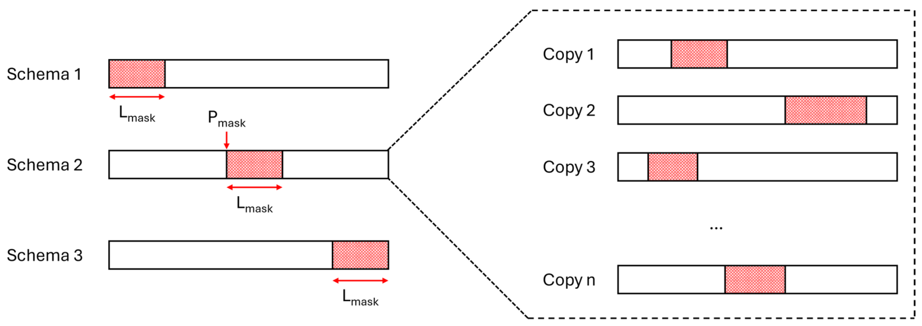
Figure 2.
Diagram of the proposed approach. Left: (1) A window containing a GPS outage section (highlighted in red) is extracted from the session. (2) GPS and fusion data for timestamps during the outage are masked by replacing values with -1 (highlighted in black). (3) The window is fed into the neural network. (4) The network outputs velocity predictions. (5) Velocities are integrated to compute positions, with an interpolation step applied to ensure smooth transitions for schema 2 (where the GPS outage occurs neither at the beginning nor end of the session). (6) Predicted positions are integrated back into the original session. Right: The architecture of the neural network.
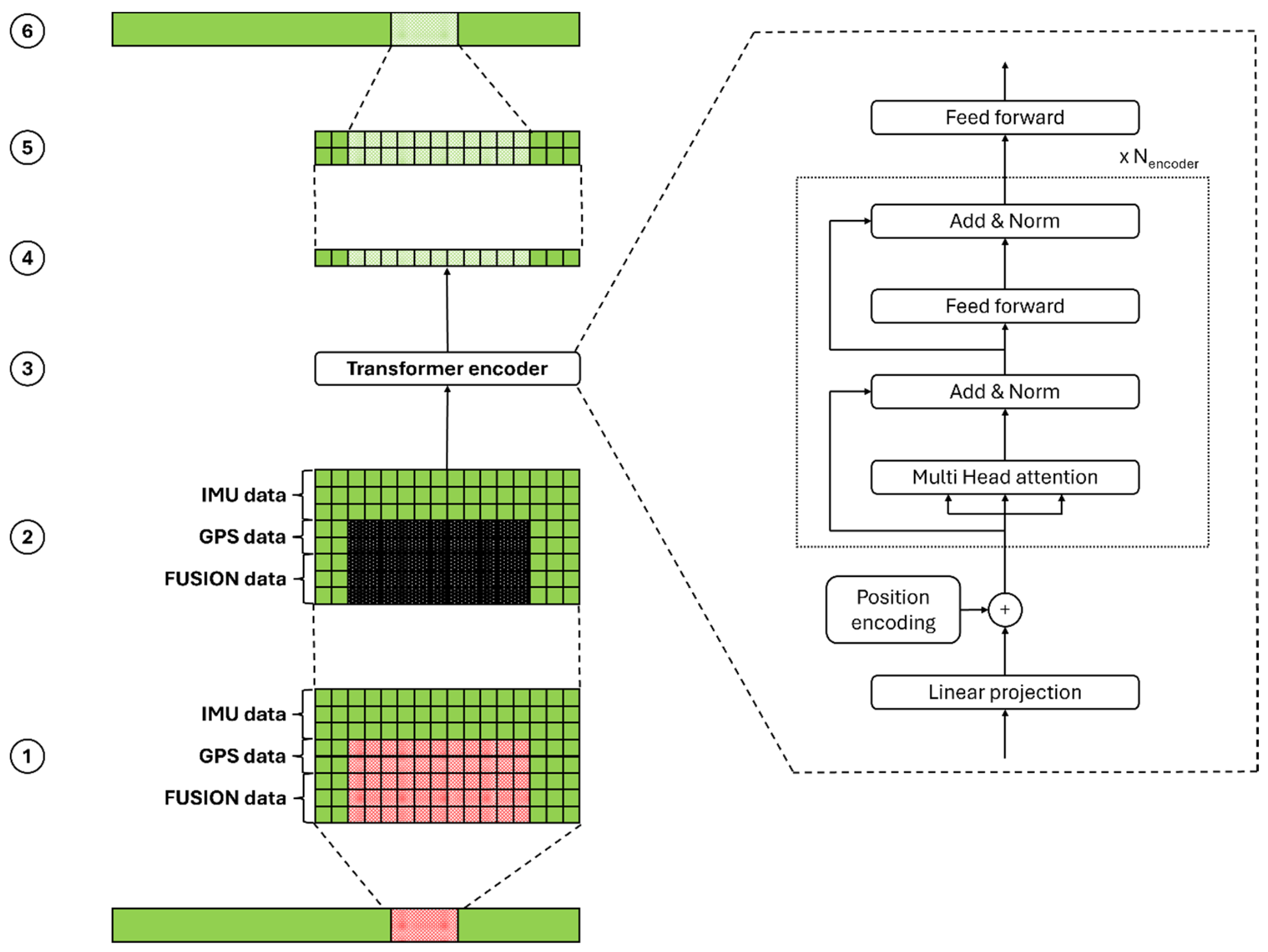
Figure 3.
Position in m (top) and velocity in m/s (bottom) distributions across the full dataset.
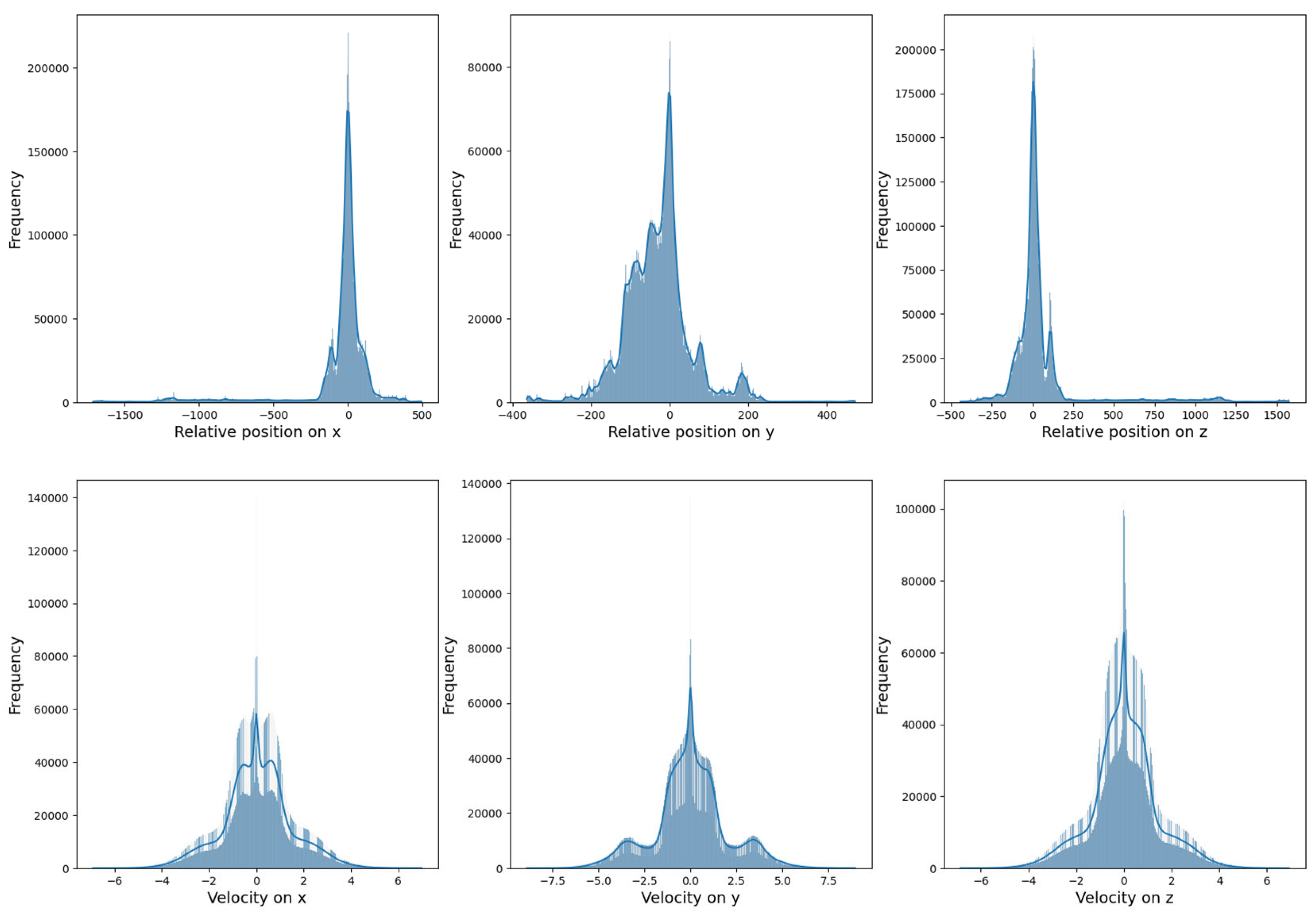
Figure 4.
Function defining tinterp based on the GPS outage duration.
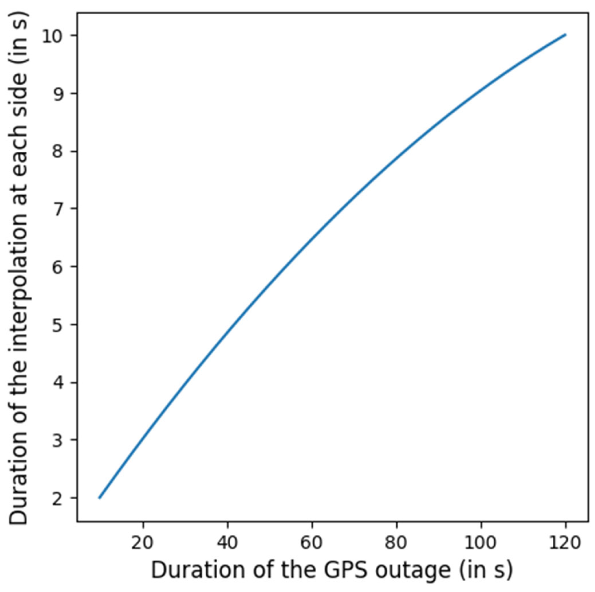
Figure 5.
Illustration of the interpolation process following bidirectional integration. Top: Quadratic interpolation functions fitted at the boundaries of the GPS outage section. Bottom: Interpolations applied to the GPS outage boundaries.
Figure 5.
Illustration of the interpolation process following bidirectional integration. Top: Quadratic interpolation functions fitted at the boundaries of the GPS outage section. Bottom: Interpolations applied to the GPS outage boundaries.
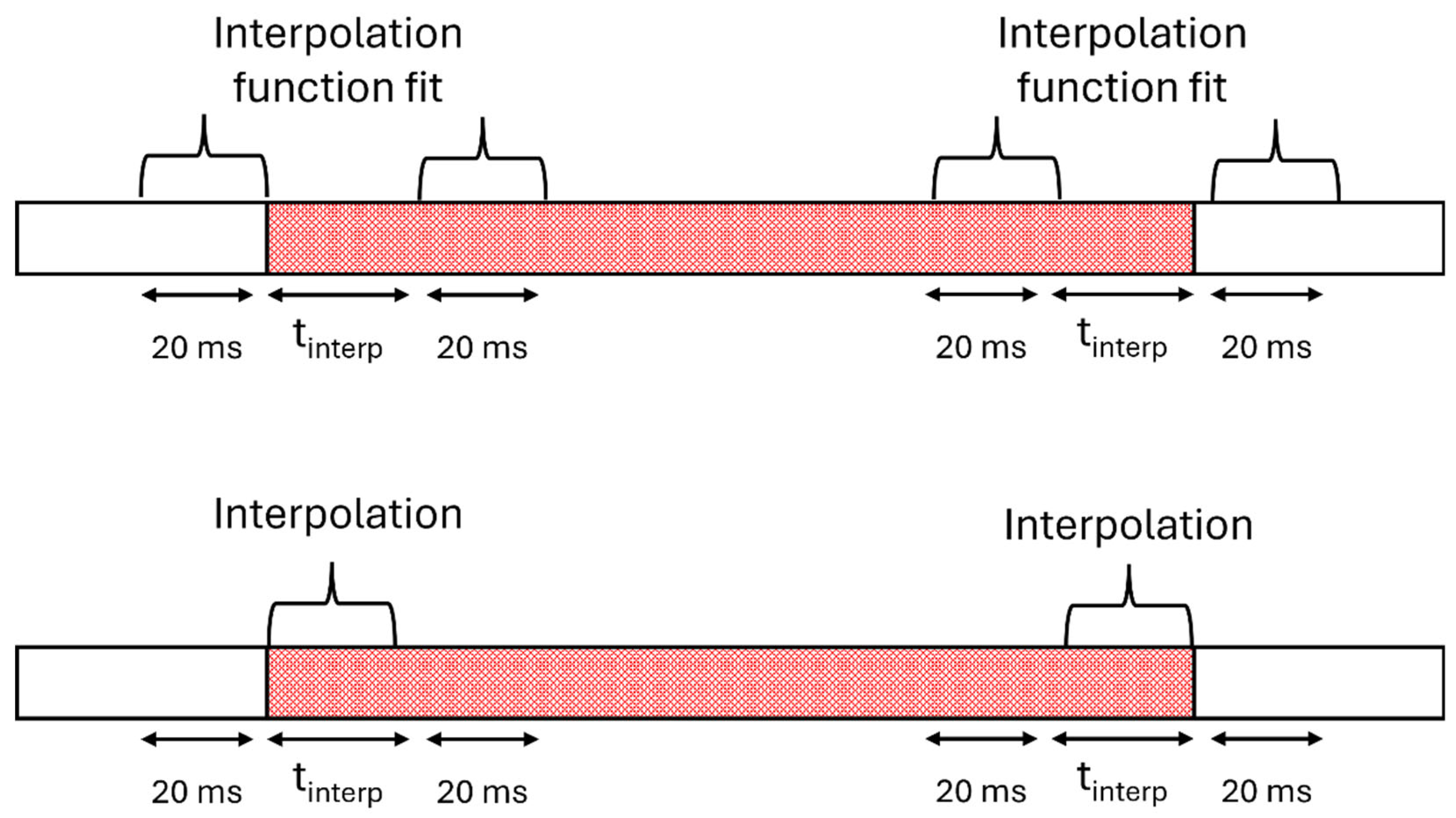
Figure 6.
Sequence extraction mechanism for training and validation.
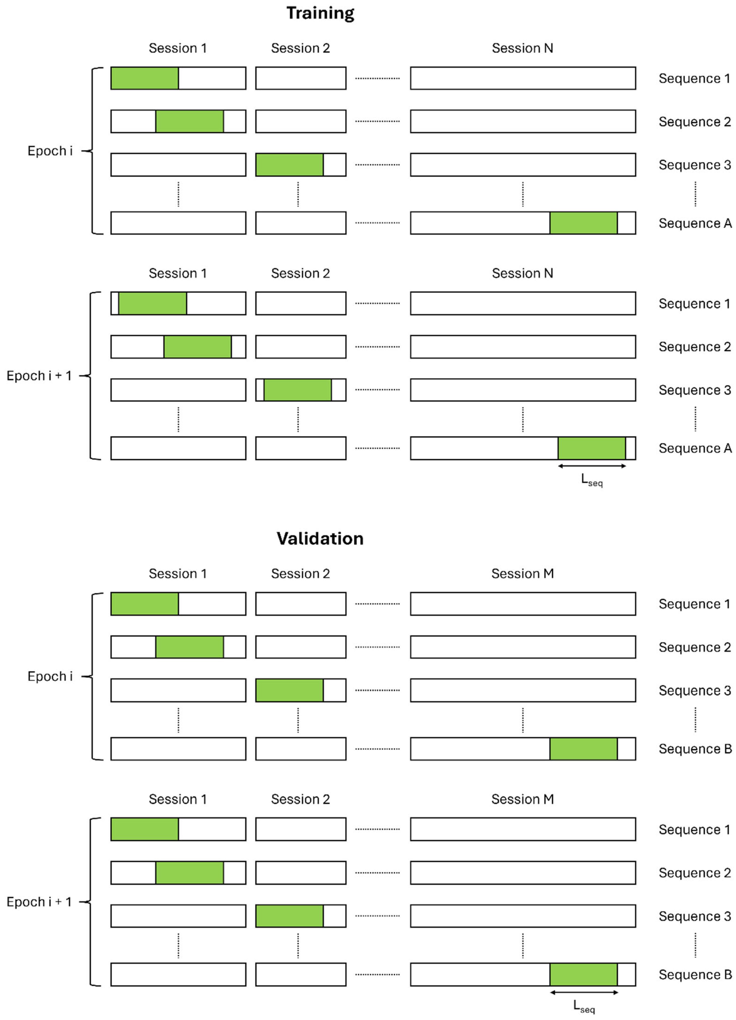
Figure 7.
Velocities (first three) and positions (last three) across three axes over time for a 38-second masked section. Green indicates the ground truth (masked before network input to simulate the GPS outage), red indicates network predictions, and blue indicates the unmasked part of the session. Positions are shown post-interpolation.
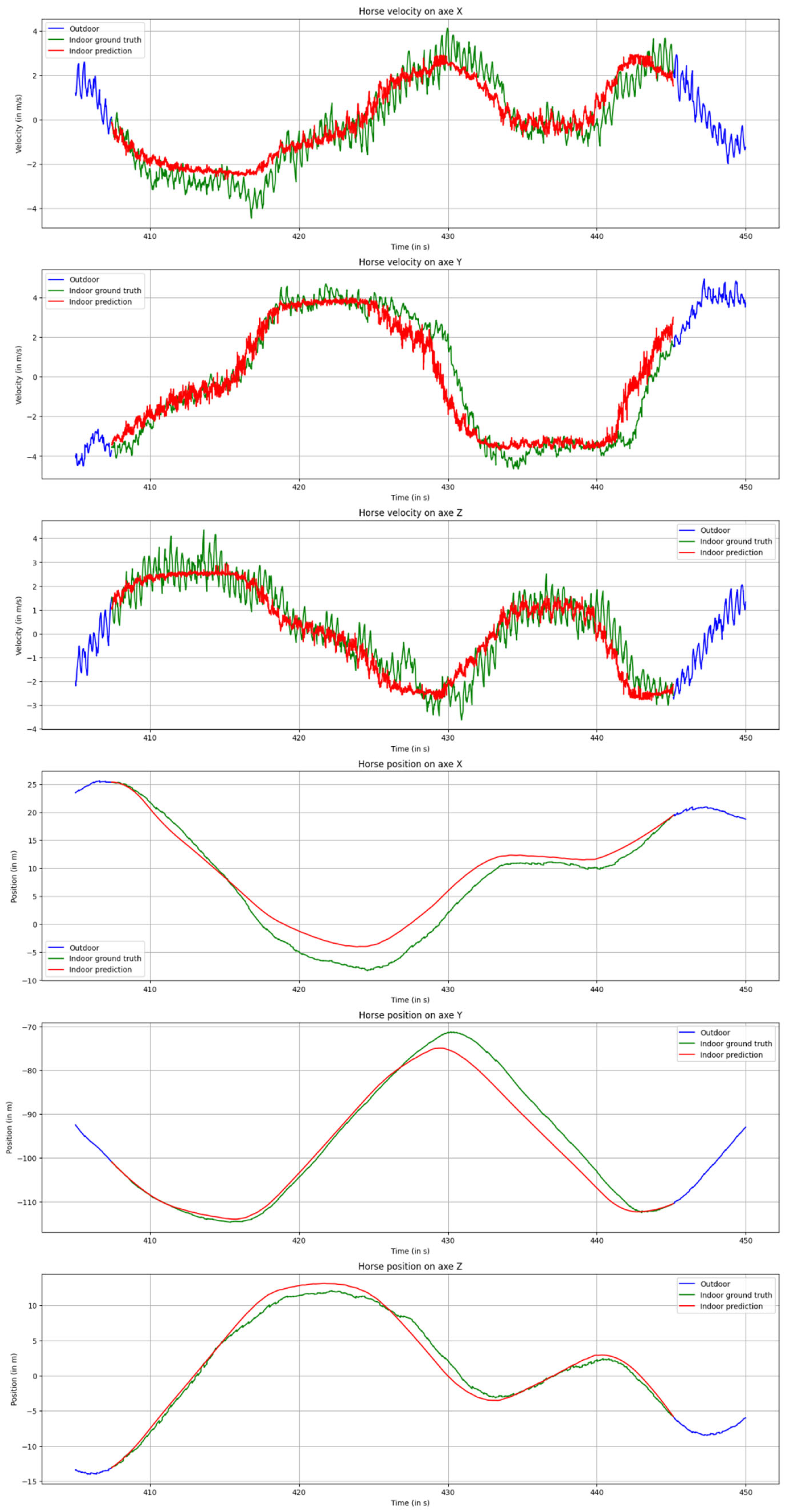
Figure 8.
Position on the x-axis versus the y-axis (top view) for a 38-second masked section. Green indicates the ground truth (masked before network input to simulate the GPS outage), red indicates network predictions, and blue indicates the unmasked part of the session. Positions are shown post-interpolation.
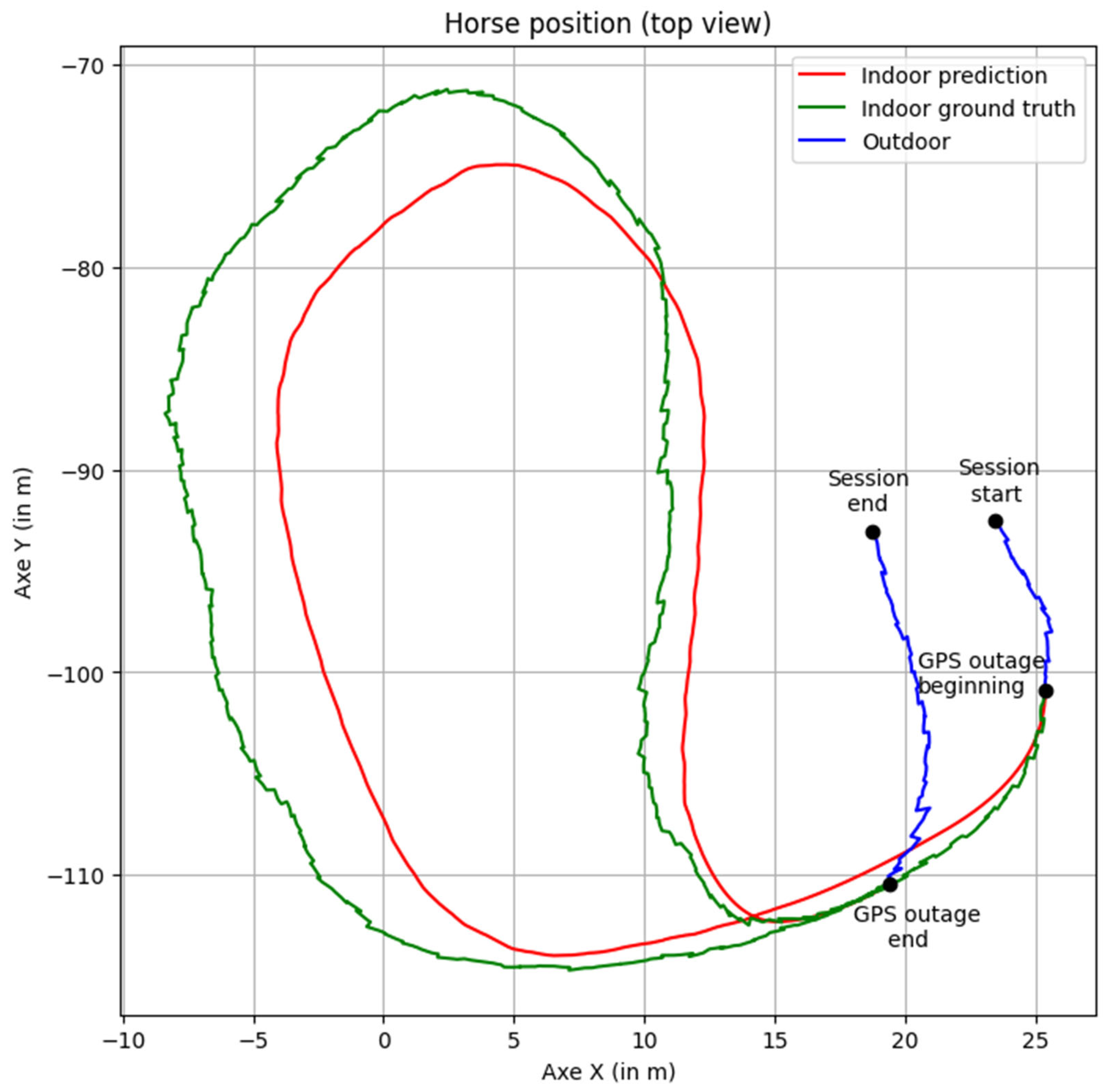
Figure 9.
Comparison of the best ATE achieved by the network across three schemas, categorized by strategies and input frequencies. Fixed strategies correspond to strategy 1 for schema 1, strategy 2 for schema 2, and strategy 3 for schema 3. The random strategy represents strategy 4 for all schemas.
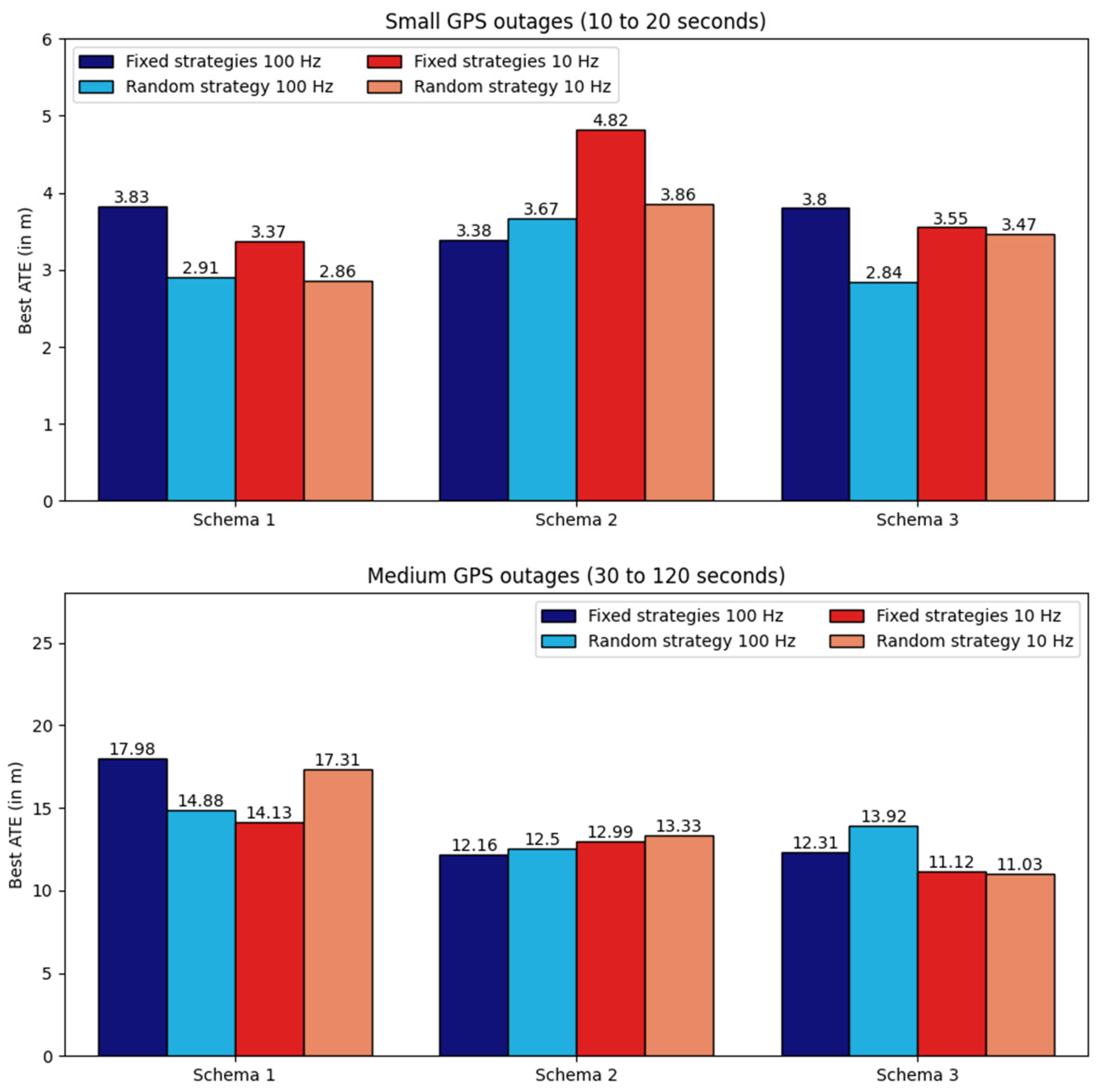
Figure 10.
Hyperparameter importance.
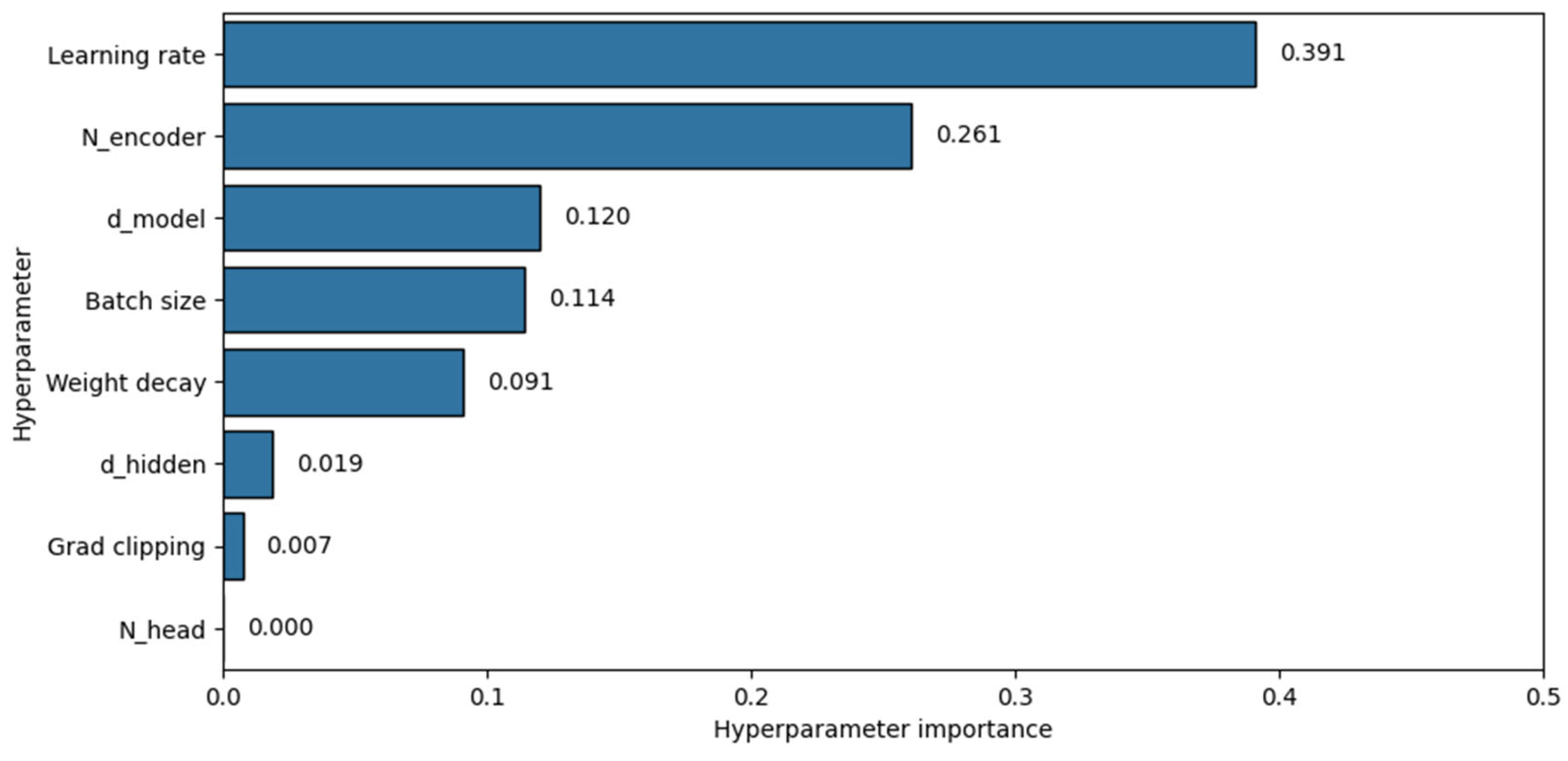
Table 1.
Hyperparameter space for the Bayesian search.
| Hyperparameter | Space |
|---|---|
| Batch size | [2, 4, 8, 16, 32, 64, 128, 256] |
| Learning rate | [1 * 10-5; 1 * 10-1] |
| Weight decay | [1 * 10-4; 1 * 10-1] |
| Gradient clipping | [True, False] |
| Gradient clipping max norm | [1; 10] |
| [0.5, 0.75, 0.9, 0.999] | |
| dmodel | [8, 16, 32, 64, 128, 256, 512, 1024] |
| Nhead | [1, 2, 4, 8, 16] |
| dhidden | [16, 32, 64, 128, 256, 512, 1024, 2048, 4096] |
| Nencoder | [1; 12] |
Table 2.
ATE, RTE, and RDE for localization reconstruction of small GPS outages (10 to 20 seconds). Results for schema 2 are presented before interpolation. The best results per schema and metric are highlighted in bold.
Table 2.
ATE, RTE, and RDE for localization reconstruction of small GPS outages (10 to 20 seconds). Results for schema 2 are presented before interpolation. The best results per schema and metric are highlighted in bold.
| Input frequence |
Schema 1 | Schema 2 | Schema 3 | ||||||
| ATE 1 | RTE 2 | RDE 2 | ATE 1 | RTE 2 | RDE 2 | ATE 1 | RTE 2 | RDE 2 | |
| Strategy 1 | Strategy 2 | Strategy 3 | |||||||
| 100 Hz | 3.83 | 0.62 | 0.39 | 3.38 | 0.20 | 0.28 | 3.80 | 0.88 | 0.32 |
| 10 Hz | 3.37 | 0.41 | 0.26 | 4.82 | 0.31 | 0.29 | 3.55 | 0.73 | 0.32 |
| Strategy 4 | Strategy 4 | Strategy 4 | |||||||
| 100 Hz | 2.91 | 0.34 | 0.35 | 3.67 | 0.20 | 0.31 | 2.84 | 0.53 | 0.30 |
| 10 Hz | 2.86 | 0.24 | 0.38 | 3.86 | 0.26 | 0.33 | 3.47 | 0.51 | 0.32 |
1 ATE is expressed in meters. 2 RTE and RDE are ratio and do not have unit.
Table 3.
ATE, RTE, and RDE for localization reconstruction of medium GPS outages (30 seconds to 2 minutes). Results for schema 2 are presented before interpolation. The best results per schema and metric are highlighted in bold.
Table 3.
ATE, RTE, and RDE for localization reconstruction of medium GPS outages (30 seconds to 2 minutes). Results for schema 2 are presented before interpolation. The best results per schema and metric are highlighted in bold.
| Input frequence |
Schema 1 | Schema 2 | Schema 3 | ||||||
| ATE 1 | RTE 2 | RDE 2 | ATE 1 | RTE 2 | RDE 2 | ATE 1 | RTE 2 | RDE 2 | |
| Strategy 1 | Strategy 2 | Strategy 3 | |||||||
| 100 Hz | 17.98 | 0.91 | 0.30 | 12.16 | 0.53 | 0.31 | 12.31 | 0.35 | 0.25 |
| 10 Hz | 14.13 | 0.73 | 0.28 | 12.99 | 0.64 | 0.30 | 11.12 | 0.23 | 0.24 |
| Strategy 4 | Strategy 4 | Strategy 4 | |||||||
| 100 Hz | 14.88 | 1.08 | 0.30 | 12.50 | 0.55 | 0.35 | 13.92 | 0.34 | 0.30 |
| 10 Hz | 17.31 | 1.18 | 0.27 | 13.33 | 0.54 | 0.30 | 11.03 | 0.28 | 0.28 |
1 ATE is expressed in meters. 2 RTE and RDE are ratio and do not have unit.
Table 4.
Optima hyperparameters subspace and best hyperparameters set.
| Hyperparameter | Optima subspace | Best set |
| Batch size | [2, 4, 8, 16, 32] | 16 |
| Learning rate | [1 * 10-5; 5 * 10-3] | 8.5 * 10-4 |
| Weight decay | [1 * 10-2; 1 * 10-1] | 1.95 * 10-2 |
| Gradient clipping | False | False |
| Gradient clipping max norm | None | None |
| [0.5, 0.75] | 0.5 | |
| dmodel | [8, 16, 32, 64, 128] | 32 |
| Nhead | [2, 4, 8, 16] | 4 |
| dhidden | [16, 32, 64, 128, 256, 512] | 64 |
| Nencoder | [1; 6] | 5 |
Table 5.
Processing time and memory consumption for inference (forward pass without gradient computation) with a batch size of 1 and for training (forward pass with gradient computation, backward pass and network optimization) with a batch size of 16. The performances have been established using the best hyperparameters found during the hyperparameter tuning phase (dmodel = 32, dhidden = 64, Nhead = 4 and Nencoder = 5) on a compute node (4 cores of AMD EPYC-7742 2.25 GHz, 40 Go of RAM and NVIDIA GeForce RTX 3090).
| Inference (batch size = 1) | ||||
| GPS outage duration |
Input frequence |
Processing time on CPU |
Processing time on GPU |
GPU memory consumption |
| small | 100 Hz | 160 ms / 1.61 ms 1 | 3.05 ms / 2.09 ms 1 | 36 Mo |
| small | 10 Hz | 4.44 ms / 217 µs 1 | 1.76 ms / 2.29 ms 1 | 32 Mo |
| medium | 100 Hz | 5.01 s / 521 ms 1 | 57.8 ms / 244 µs 1 | 54 Mo |
| medium | 10 Hz | 49.0 ms / 822 µs 1 | 1.80 ms / 2.21 ms 1 | 34 Mo |
| Training (batch size = 16) | ||||
| GPS outage duration |
Input frequence |
Processing time on CPU |
Processing time on GPU |
GPU memory consumption |
| small | 100 Hz | 8.42 s / 28.0 ms 2 | 30.9 ms / 1.43 ms 1 | 304 Mo |
| small | 10 Hz | 172 ms / 5.35 ms 2 | 16.2 ms / 1.40 ms 1 | 74 Mo |
| medium | 100 Hz | None 3 | 527 ms / 1.81 ms 1 | 1448 Mo |
| medium | 10 Hz | 4.15 s / 40.0 ms 2 | 19.1 ms / 1.69 ms 1 | 184 Mo |
1 Mean / standard deviation of 20 loops of 100 repetitions each. 2 Mean / standard deviation of 20 loops of 10 repetitions each. 3 Total computation time for 200 repetitions greater than 12 hours or memory requirements superior to the configuration.
Disclaimer/Publisher’s Note: The statements, opinions and data contained in all publications are solely those of the individual author(s) and contributor(s) and not of MDPI and/or the editor(s). MDPI and/or the editor(s) disclaim responsibility for any injury to people or property resulting from any ideas, methods, instructions or products referred to in the content. |
© 2024 by the authors. Licensee MDPI, Basel, Switzerland. This article is an open access article distributed under the terms and conditions of the Creative Commons Attribution (CC BY) license (http://creativecommons.org/licenses/by/4.0/).
Copyright: This open access article is published under a Creative Commons CC BY 4.0 license, which permit the free download, distribution, and reuse, provided that the author and preprint are cited in any reuse.


