
Submitted:
13 November 2024
Posted:
13 November 2024
You are already at the latest version
Abstract
Air pollution represents one of the most complex problems of the modern industrialized world, as, practically, all sectors of human activity can be sources of polluting emissions and greenhouse gases. In this context, traffic must be remembered as having a significant contribution to this, although active and passive technologies have been implemented to reduce fuel consumption and emissions, but the increase in the number of vehicles in traffic has almost canceled these reductions. Air quality in urban areas is generally monitored with specialized equipment in fixed measuring stations without a selective analysis of the origin of the pollutants, so when the tolerance limits of the pollutants are exceeded, the car is generally unfairly penalized, due to the fact that the traffic road is a source of pollution visible to anyone compared to other sources, such as: industry, agriculture, energy, domestic heating, construction, road infrastructure maintenance operations, and other ones. This paper primarily presents the influence of different classic propulsion systems in relation to the geometry of the road infrastructure and the characteristics of urban road traffic where there is a high frequency of changes in the dynamics of vehicle movement on the levels of polluting emissions and fuel. In addition, the influence of various factors on emissions and fuel consumption in extra-urban road traffic conditions is also examined. The objective of the research carried out and presented in this paper clarifies some aspects regarding the participation of motor vehicles in air pollution and targeted three aspects with different weights in terms of importance:
1) to collect real data on fuel consumption and emissions of cars in traffic in the city of Brașov (RO) and its surroundings;
2) to gain insight into the relationship between fuel consumption and emissions, on the one hand, and road traffic characteristics, on the other hand;
3) to gather the necessary data for the realization of a real road traffic simulation tool incorporated in a test driving cycle for bench testing in the laboratory by which one can evaluate the behavior of any car in traffic and compare it with other vehicles and, through simulating traffic on different driving conditions, fuel consumption and emission levels through road traffic management interventions could be reduced. This phase represents the essence of this paper as it is based on the data collected in real urban and extra-urban traffic conditions by using the "Driving Cycle" software available at the test bench, consequenly, the urban and extra-urban test driving cycles containing the maps will be modeled (speed, time, speed change, road gradient, etc.) identically to the data recorded in real traffic. By identifying routes that represent the characteristics of traffic flows and (traffic volume, traffic light phasing, regulatory strategies and so on) representing traffic in urban and extra-urban areas and by transposing these routes in test cycles in the laboratory, it will be possible to analyze the behavior of any type of vehicle in terms of fuel consumption and traffic emissions.
Keywords:
Fuel Consuption
; Pollutant Emissions
; Driving Cycles
; Test Cycles
1. Background
Over recent decades, the modern world has faced an increase in the number of personal vehicles per capita (considered as motorisation indicator), which serves as the main way of transporting people and goods, both in developed countries and in many developing countries.
This trend can be related to the increase in the income of the population and the increased mobility needs of households. The analyzes carried out show that there are other factors that contribute to the increase of the indicator named vehicles per capita, namely: the availability of quality road infrastructure, the offer and provision of efficient services by public transport, policy decisions affecting vehicle ownership such as: taxation rules and insurance levels, car cost policies, policies regarding the price of fuels and lubricants, costs and, the last but not least, the decisions regarding the expenses associated to alternative modes of transport, [24,25,26,27,32,33,34,35].
EU member states reported an average increase of 14.3[%] in car motorization rates over the last 10 years (2012–2022), with the highest increase being recorded in Romania (86.2[%]), reaching a number of 417 cars per 1000 inhabitants, compared to 560 cars per 1000 inhabitants, the average value in the EU, and Italy had the highest number with 684 passenger cars per 1 000 inhabitants, [37,38,39,40,41,42].
The increase in the number of vehicles indicates a certain level of development of society and a high standard of living, fact that brings with it a large number of disadvantages that can have adverse effects on the standard of living. First of all, the urban road infrastructure was designed and built, in many cities, a long time ago, this fact causes congested traffic, difficult to manage the traffic, and the result is reflected in low travel speeds. Secondly, the large number of vehicles in congested traffic causes high fuel consumption and increased levels of polluting emissions (NOx - nitrogen oxides, CO – carbon monoxide, HC- hydrocarbons and PM – particulate mattj n ner) and greenhouse gases (CO2 - carbon dioxide, N2O - nitrous oxide, etc.).
It should be noted that during the same period in which the number of vehicles increased, a great diversity of vehicle propulsion systems appeared in response to the regulations regarding the protection of the environment. So, at this moment, vehicle propulsion systems can be divided into three broad categories in various configurations: 1) classic propulsion system vehicles (spark ignition engine vehicles - SIEV, compression ignition engine vehicles - CIEV), 2) vehicles with electric hybrid propulsion systems (HEV) and, 3) vehicles with electric propulsion systems (BEV).
The analysis of the structure in the Brasov region (RO) vehicle fleet shows that it is predominantly equipped with classic propulsion systems, i.e. an internal combustion engine (petrol engine or diesel engine) associated with a manual gearbox or automatic gearbox. The number of vehicles with electric propulsion systems (full hybrid, plug-in hybrid and electric vehicle with battery) is relatively small but has a dynamic growth in the future [36] .
Over time, the test driving cycles in different areas of the world (North America, Europe and Asia) have evolved due to changes in traffic and the emission limits related to testing with the cycles in force have been continuously decreasing. The last major change in the field imposed a harmonized test cycle of vehicles, valid all over the world, to which regulations regarding emission and consumption limits are applied. In order to be put into circulation, vehicles must be homologated, for this process they are subject to the WLTP (Worldwide Harmonized Light Vehicles Test Procedure) test driving cycle, which is a cycle with global applicability and involves testing vehicles in laboratory conditions with driving similar to traffic real-world driving that includes accelerations, decelerations and variable speeds, and then, by measuring pollutant emissions and fuel consumption during the cycle and comparing them to regulated limits provides an insight into the vehicle’s environmental performance under standardized test conditions. The WLTP test cycle was built on the basis of real recorded data describing urban and extra-urban road traffic for all categories of vehicles under general conditions accepted by all countries of the world [1].
The imposition by successive legislative regulations of increasingly strict limits on the emissions of vehicles equipped with internal combustion engines have determined serious concerted actions by the main actors in the field (research-development, manufacturing) to implement active and passive technologies so that the engines correspond to the limits in force at that time[1]. The stages of the legal framework regarding vehicle emissions in the European Union have been standardized under the name Euro 1(1992), Euro 2(1996), Euro 3(2000), Euro 4(2005), Euro 5(2009), Euro 6(2014), Euro 7 (2024). In order to meet the requirements for limiting emissions, a series of active technologies were successively implemented, aimed at reducing the rate of formation of polluting substances and reducing fuel consumption, and passive technologies for treating exhaust gases. Active technologies have been applied to both types, spark ignition engine (SIE) and compression ignition engines (CIE) of engines with their specificity, as follows; the gas exchange systems (variable gas distribution systems) and fuel systems were improved (injection systems with electronic control were introduced for both types of engines), the use of quick-response sensors, on-board diagnostics (OBD), the exhaust gas recirculation (EGR), the improved engine performance control systems, the use of variable geometry turbochargers, etc[1,2,5]. Passive technologies applied to the treatment of exhaust gases have undergone changes aimed at increasing the pollutant conversion rate, especially at low exhaust gas temperatures and in the case of net oxidizing burnt gases (the case of engines that use lean air-fuel mixtures) [4,15].
The emissions of vehicles with internal combustion engines are dependent on the processes that take place during engine operation, generally characterized by parameters such as: engine load determined by the nominal power delivered, which is proportional to engine speed and torque, thermal state of the engine[21,22,23].
The thermal state of the engine is indirectly assessed by a set of temperatures of some environments that operate in its systems, e.g. coolant and lubricating oil [14]. The influence of the thermal state of the internal combustion engine on the emission of pollutants in the air in traffic manifests itself more intensively in the engine warm-up phase, up to a certain constant temperature established by the engine manufacturer [3]. After stabilizing the thermal state of the engine, the level of polluting emissions depends mainly on the speed and torque of the engine, which are also the parameters that concern the traction of the vehicle, and on these conditions the traction of the vehicle can be determined by the speed of the car [9,10,11,12,13,14].
Evaluating the share of pollutants released by each source of pollution to this global pollution at the level of a city presents a major difficulty, as it requires environmental studies for rigorous analyzes or emission factors are used that appreciate the participation of each source. In general, without an analysis of the contribution of each source to the global air pollution in the urban area, the source invariably incriminated by some citizens, the media and politicians is the road traffic (as mobile source), because it is visible and there are also some negative effects of it (agglomeration , low travel speeds and frequent stops at traffic lights, noise, etc.) despite the fact that vehicles in recent years have adopted effective depollution devices [16,17].
Over time, numerous scientific studies were carried out and were dedicated to researching the impact of pollutant emissions on the environment, especially analyzing traffic flows and ways to improve them [5,6,7,8,28,29,30,31,32,33,34,35,36].
The "Integrated Air Quality Plan in the Municipality of Brașov for PM10 and NO2 /NOx 2023 - 2027" made by the authorized bodies (Brasov City Hall and the Environment Agency of the city of Brasov) [43], provides data on pollutant emissions of NOx and particles from different sources in previous years, and the trends and measures to be applied.
The regulations in force provide the following thresholds for the concentration of Nitrogen Oxides (NOx) in the atmospheric air:
- -
- Limit values 200 [μg/m3] NO2 - the hourly limit value for the protection of human health;
- -
- The annual limit value of 40 [μg/m3] NO2 for the protection of human health; and
- -
- Critical Level of 30 [μg/m3] NOx - for protection of fauna and flora;
In Figure 1. the maximum values of the NOx concentration in the air recorded by the air quality monitoring stations in Brașov are presented.
In this plan, the distribution of NOx concentration at the level of Brașov municipality in 2019, as a reference, calculated with the COPERT program, was as follows: static sources =12.71[%], surface sources = 14.02[%], mobile sources = 73.27[%].
In the field of transport, the vehicle is considered a mobile source of pollution that discharges gaseous pollutants into the atmosphere: NOx, CO, HC and PM 2.5 solids which are found in the pollutants monitored by urban measuring stations for air quality
In this plan, the mobile sources of pollution are represented by the following categories of vehicles equipped with internal combustion engines: cars, vans, heavy vehicles including buses and motorcycles.
Within the category of mobile pollution sources, the distribution of NOx calculated with the same COPERT program for each vehicle class is as follows: passenger cars = 30[%], vans = 16[%]. heavy vehicles including buses = 53[%], and motorcycles = 1[%.]
The CO2 emission must be analyzed carefully, because, most of the time, the transports, which include road transports, are criminalized as belonging to the category of large emission sources. Nevertheless, it is not taken into account that, in recent years, solutions have been implemented in vehicles that have aimed at reducing fuel consumption in order to reach the CO2 emission target, the increase in the share of the global emission of the transport sector belonging to road transport is mainly due to the increase of the number of vehicles.
2. Methodology
2.1. Experimental Framework
The experimental tests have as the main objective the modelling of a vehicle driving cycle, based on real experimental data obtained on routes that comprise global urban and an extra-urban traffic. These cycles will be implemented in the dynamometric stage memory to test other vehicles on the same traffic conditions and to compare the results regarding emissions and fuel consumption.
- In order to achieve this objective, the experimental research will be carried out in three stages:
- In the first stage, data will be collected regarding traffic characteristics, emissions, and fuel consumption on the routes selected for the vehicles under consideration.
- In the second stage, the data recorded on the chosen routes are entered as input data in the Driving cycle software of the dynamometric stand to obtain the real driving cycles that represent the research objectives.
In the third stage, the selected vehicles are tested on the dynamometric stand using the driving cycle obtained in the previous stage.
For validation, the values of emissions and fuel consumption obtained with the measuring equipment provided on board of the vehicles when travelling in real traffic are compared with the values measured for emissions and fuel consumption by the dynamometric test stand equipment (Figure 2).
2.2. Analysis of Representative Test Routes
The process of choosing the research routes requires a very careful analysis because they must be representative for the city of Brasov and the adjacent areas. The difficulty lies in the fact that some streets were laid out a few hundred years ago and others a few decades ago, and on these streets, which have a limited width, a huge number of vehicles travel. Another characteristic is represented by the wide variety of restrictions without adequate management that affect traffic flows, such as: intersections controlled by traffic lights, intersections controlled by signal boards, intersections controlled by roundabouts, pedestrian crossings controlled by traffic lights, crossings of pedestrians controlled only by signal boards, bus stops, etc.
When selecting the routes for the tests, it was considered that they should be representative for the city of Brasov and respond to the transport needs for population and for goods to reach administrative institutions, kindergartens, hospitals, economic units (production, sales, etc.) and, not in the end, making connections with other transport routes. To achieve this goal, a traffic study was initiated and carried out.
The mixed route is 5.4 km long and includes both low and higher travel speeds (the travel speed was respected throughout the tests according to the restrictions encountered). The starting point is on Castelului str. (one-way street) and continues on Politehnicii str. (one-way street), Nicolae Balcescu str. (two-way street), 15 Noiembrie Bd. (one-way street), Agriselor str. (one-way street ), Iuliu Maniu str. (two-way street ), A.I. Cuza str. (two-way street ), Avram Iancu str. (two-way street ), Stadionului str. (two-way street), Calea Fagarasului (two-way street), Fanarului str. (two-way street), Institutlui str. (two-way street), return point (Institute of Research and Developpement), Fanarului str. (two-way street), Curmaturii str. (two-way street), DN 73 (two-way street), Ioan Clopotel str. (two-way street), Brasov Belt E574 (one-way street) (Figure 3a).
The selected mixed route is characterized by a high uncertainty regarding stops at pedestrian crossings signaled by warning signs that depend on the intensity of pedestrian traffic and at intersections with roundabouts that depend on the intensity of vehicle traffic entering the intersection from adjacent streets . Consequently, travelling this route can generate 34 stops, of which 30 stops can be of variable duration (20 pedestrian crossings, 2 intersections without traffic lights and 8 roundabouts) and which cause variations in perceptible intervals of travel speed, fuel consumption fuel and emissions, and weather changes can amplify or diminish these variations as well.
The route selected to generate the real extra-urban driving cycle was selected outside the town, being a part (7.1 km) of the Brașov city belt (Figure 3b). Along the extra-urban route, there are five roundabouts that intersect secondary roads with a relatively high flow of vehicles at peak hours (this flow is high in the morning hours from outside the city to the city center and vice versa, from the city to outside areas.
The study of the behaviour of vehicles in extra-urban traffic is imposed by the bypass belt of the city of Brasov which is placed nearby and which supports the traffic of vehicles of all categories in transit to other localities and which partially influences the state of the environment in the city.

Table 1.
Characteristics of routes selected to generate the proposed actual driving cycles (mixed cycle and extra-urban cycle).
Table 1.
Characteristics of routes selected to generate the proposed actual driving cycles (mixed cycle and extra-urban cycle).
| Route Characteristics | Mixed Route | Extra-urban Route |
|---|---|---|
| Traffic lighted intersections | 3 | - |
| Roundabout circulation | 8 | 5 |
| Intersections directed by road signs | 2 | 1 |
| Pedestrian crossings with traffic lights | 1 | - |
| Pedestrian crossings without traffic lights | 20 | 2 |
| Brasov bypass exits/entrances | - | 3 |
2.3. Test Vehicles and Their Characteristics
The tests were carried out on a number of 4 new generation vehicles (SUV, Sedan and Van), having the Euro 6 pollution standard which is representative for urban traffic.
Table 2 shows the technical characteristics of the vehicles, which constitute input data for the software used during the tests on the dynamometer stand.
Due to fleet renewal programs, the vehicles in traffic are relatively new, the average mileage of the vehicles chosen for testing is 31.500 [km], the maintenance work on these vehicles was carried out on time by authorized specialized car units. On these conditions, hidden defects on car engines are excluded; therefore, the results obtained on pollutant emissions and fuel consumption were not influenced in any way by other factors.
2.4. Traffic Conditions
The chosen routes for our research study were travelled on four weekdays during peak traffic conditions between 11:30 a.m. and 1:00 p.m.
Traffic studies have identified that in this time interval the intensity of traffic increases, reaching the figures of the morning and evening peak hours, this intensification of traffic is generated by the pick-up of young students from schools and kindergartens and by the traffic during the lunch break. Rush hour traffic is characterized by congestion, low travel speeds that can generate negative effects on emissions and fuel consumption.
2.5. Modelling of the Real Driving Cycle
Mathematical modelling is an essential tool in scientific research, providing a robust framework for understanding, analyzing and forecasting complex phenomena in various fields. The mathematical model used has the potential to contribute to the specification of the impact or the benefits brought, such as improving the understanding, efficiency or solutions for the problems identified regarding the parameters that directly influence the pollutant emissions and fuel consumption in the case of the tested vehicles.
This paper presents a mathematical model used by the "Driving Cycle" software, which is implemented in the dynamometric stand calculation system used for road tests, intended for the creation of new test driving cycles using real data collected in traffic on a predetermined route, to be used to understand and analyze the graphics made with the help of a calculation algorithm based on tables in different formats (Excel, Notepad, csv.) and which later performs the modelling using AutoCad 2023 software.
The forces that determine the dynamics of the vehicles being tested on the stand are calculated using the dynamometer software library by inputting the requested customized data of the target vehicles.
F - Value of traction load (constant),
Cf A - Rolling resistance coefficient (constant),
Cf B – Flexible power coefficient (linear),
Cf C – Air resistance coefficient (n≈2),
Cf D - Air resistance coefficient (with variable n exponential),
exp. D – Exponent D(1 ≤ n ≤ 3)
mautov – Mass of the vehicle
mrol - Mass of the dynamometer rollers (moment of inertia of the rollers reduced to the translational movement),
v – Roller speed.
dv/dt – Acceleration of the rollers,
g - Gravitational acceleration,
α – Angle of inclination (+⁄-).
A reference speed (90[ km/h]) will be chosen for coefficients Cf A and CfD.
a) The rolling resistance coefficient Cf A [kW].
In the second phase, the resistance power of the roller (2) will be calculated, and derives from changes at the level of the tire and the road surface depending on the speed of the vehicle.
where: µr = 0.012 (Coefficient of adhesion of the tire with the stand roller), m = 1050 kg (Mass of the vehicle),
g = 9.81 [m/s2] (Gravitational acceleration)
v = 100 [km/h] (Travel speed), 100∙1000/3600 = 100∙ 0.277=28 [m/s]
Cf A = 0.012 · 1050 · 9.81 · 28 = 3.46 ≈ 3.5 [kW]
This represents a small value of the total road load and a standard value will be adopted for radial tires ≈2.5 [kW] and winter tires ≈3.75 [kW].
b) Flexible power factor (Cf B)
The calculation of the power coefficient is the next phase and it represents a linear component of the rolling resistance power for a reference speed. This coefficient is defined as the power loss that occurs when the tire flexes on the road or roller surface.
In general, the value of this coefficient does not significantly change the test results due to the minimum resistance coefficient of the tire’s flexibility.
c) Air resistance coefficient (n≈2) Cf C
This coefficient is directly proportional to the front surface of the vehicle and the resistance coefficient cw.
where: ρ = 1.1 [kg/m3] – Air density,
aw=0.38 – Air resistance coefficient,
frontal = 1.77[m] ∙ 1.55[m]=2.743 [m2]≈2.7 [m2] – Frontal area of the vehicle (l x h),
v = 100 [km/h] = 28 [m/s] – Travel speed
v0= 0 [km/h] = 0 [m/s]
Cf C = 0.5∙1.1∙0.38∙2.7∙〖28〗^2∙28= 12.387 [kW] at 100 [km/h].
Cf C = 12.387 [kW].
d) Vehicle mass "m" [kg].
Determining the coefficients based on the characteristic parameters of the tested vehicles and inserting the obtained data into the stand program are necessary to initialize the load modelling according to each vehicle.
In the lines below, some of the calculation formulas used by the analyzer software [14] will be presented. To find out the carbon dioxide in the exhaust gases, the following formula will be used.
CO2 = Carbon dioxide [%],
CO2max= The characteristic parameter of the fuel used (SIE = 15.4 [%] and CIE = 15.7 [%]),
O2 = Oxygen content of exhaust gases.
During the combustion process that takes place in the Diesel engine cylinders, in addition to NO (nitrogen oxide) already formed, NO2 (nitrogen dioxide) is also present. The concentration of NOx (nitrogen oxides) can be calculated as the sum of the concentrations of NO and NO2. The nitrogen oxide measured in the exhaust gases can reach a percentage of up to 95% of the total NOx (the remaining 5% remain for NO2). The formula for NOx used by the analyzer is [14]:
where:
NOx = Nitrogen oxides[ ppm],
NO = Nitric oxide [ppm].
The concentration of a certain substance such as CO (carbon monoxide) regarding the oxygen content can be described by the formula below [14].
where:
COrel = Carbon content in relation to oxygen,
O2ref = Reference oxygen, conventional parameter, chosen according to the fuel [%],
O2meas = Oxygen content measured in exhaust gases [%],
20.95 [%] = Oxygen concentration in pure air,
CO = Total concentration of carbon monoxide (absolute concentration).
The formula [14] is used for the concentration of undiluted carbon dioxide (COned):
CO ned= CO ⋅ λ
CO = Carbon monoxide concentration (parts per million),
λ = Coefficient of excess air.
The excess air coefficient (λ) is ratio of the amount of air entering the engine cylinders at the end of the intakes troke to participate in combustion of 1 [kg] of fuel relative to the amount of air required to burn one kilogram of fuel and is calculated according to the formula:
where:
L= The amount of air entering the engine cylinders at the end of the intake stroke participating in combustion of 1 [kg] of fuel,
Lmin= The amount of air required to burn one kilogram of fuel.
or,
CO2 = Carbon dioxide [%],
CO = Total concentration of carbon monoxide (absolute concentration) [%],
O2 = Oxygen content measured in exhaust gases [%],
HC = Unburned hydrocarbons [ppm].
The amount of air required for the complete combustion of one kilogram of fuel can vary depending on the type of fuel, namely, for the combustion of gasoline, the stoichiometric ratio for air is approximately 14.7 kilograms of air. It is important to note that these calculations are theoretical and may vary depending on the actual combustion conditions (such as pressure, temperature, etc.) and the exact composition of the fuel, and in practice, a varied ratio may be obtained depending on the specific conditions of the combustion process.
3. Measurement Equipments
The experimental research was carried out in two phases, in the first phase, the outdoor one, data were collected that focused on the characteristics of road traffic on the chosen routes, in the second phase, the indoor one, the targeted vehicles were subjected to have a simulated traffic research on the stand based on the test cycle, generated and implemented on the stand with the collected data in the first phase (Figure 2).
3.1. On Board Measurement System
To measure and store fuel consumption data, a BC 3329 on-board computer connected to an AIC1200 fuel flowmeter mounted on the vehicle’s fuel supply circuit was used Figure 4. The data from the flowmeter are transmitted to the BC 3329 on-board computer, they are stored and provided in tabular format (csv.) with the possibility of processing them.
The assembly diagram of the fuel consumption measurement system on the vehicle is presented in Figure 5a, for gasoline vehicles and Figure 5b, for diesel powered vehicles. As can be seen in Figure 5a, in the case of the SIE it is used the pressure regulator mounted before the fuel flow meter, and in the case of the CIE (Figure 5b) a fitting (M16x1.5/ s380 100) for return of excess fuel from the engine is used.
The data provided by the on-board computer are stored on a memory stick (csv.) so that they can later be analyzed in parallel with the data provided by Portable Emission Measurement System for emissions.
In the first phase of the experimental research, the tests were carried out on the road (transient regime) on a predefined route, and the data depending on the speed, time, the thermal regime of the engine, the temperature of the aspirated air and the calculated load value could be recorded with the help of the software diagnostic Bosch KTS 560.
The values of NOx, CO and CO2 emissions are recorded with the GA 21 Plus portable gas analyzer, and the fuel consumption with the AIC 1200 Series fuel flowmeter providing the data to a Board Computer BC 3329.
3.2. Dynamometric Bench for Measurement in the Laboratory
During the experimental research, equipment was used to obtain the necessary data for the analysis of emissions and fuel consumption, such as: the Maha LPS 3000 dynamometer stand, the Madur GA21 Plus Gas Analyzer, the AIC 1200 fuel flowmeter (transferring the recorded data to a Board Computer, BC3329 LOG 20 ) and car diagnosis Bosch KTS 560 model.
The Madur GA 21 Plus gas analyzer model is subject to periodic calibrations in accordance with SR EN ISO 9001:201 and SREN ISO/CEI 17025:2018, in order to maintain the accuracy of the measured data [19,20].
The possibilities offered by the gas analyzer regarding the measurement data are numerous and with a possibility of modelling in different formats, namely: data recording/viewing can be done both in graphic and tabular format, both can be inserted/saved under other extensions, e.g. - from csv. to Excel, from Excel to SPSS, etc.
The values of the measured emissions are rich and the accuracy of the results is very high. Carbon monoxide (CO), nitrogen oxide (NO), nitrogen oxides (NOx), unburned hydrocarbons (HC), carbon dioxide (CO2) and the lambda parameter (λ) are just some of the quantities that can be analyzed both in tabular and graphic format. The recording/storage time of these values is once every 2 seconds.
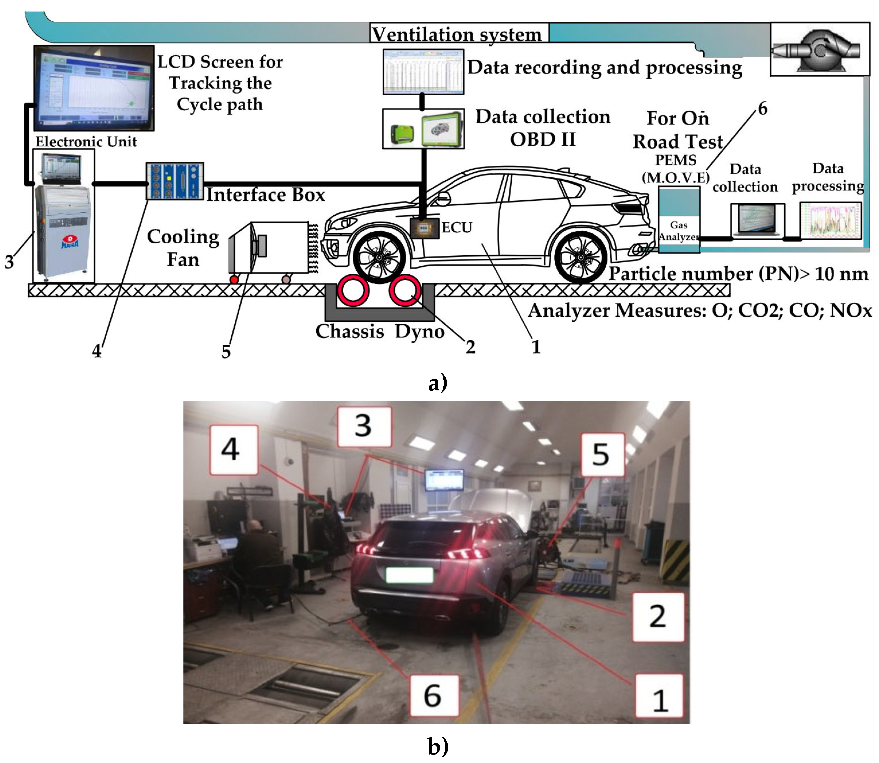
Figure 6.
Organization of the Maha LPS 3000 dynamometer stand: a) Scheme of the research stand; b) View of the research stand; 1.Tested vehicle, 2. Rollers with eddy current braking systems, 3. Control system, 4. Connection box with vehicle system (OBD II), 5. Fans (2 pieces), 6. Analyzer sampling probe [16].
4. Analysis of Experiments and Results
4.1. Real Modelled Driving Cycle
In the first stage of the experimental research, the main purpose is the collection of data when driving on the selected routes to generate the real driving cycles necessary for the research of the behavior of the vehicles selected in the first phase and of others depending on the needs of the subsequent research. Since the selected routes have a vehicular and pedestrian traffic sign that introduces a series of uncertainties regarding the speed and travel time of these routes, it was decided that the two routes (mixed and extra-urban) should be covered four days a week in the same time interval to choose the convenient travel option to obtain a real usable driving cycle for the city of Brasov.
The experimental research on data collection with the help of the portable emissions measurement system (PEMS) by travelling the two selected routes was carried out in four days of the week during the same time intervals.This approach highlights the influence of traffic intensity, stops at pedestrian crossings due to their presence and stops at intersections with other streets.
In the second stage of the research, the experimental data collected during running on the selected routes were carried out, the tests that were carried out in the special laboratory set up on the dynamometer bench after a cycle in which the conditions were reproduced in a similar manner to those carried out in real traffic through the processing of the collected data are inserted in tabular format according to speed and time, thus obtaining maps that, through the bench software, more precisely the Driving Cycle option, create the real driving cycle that will be able to use subsequent tests on the dynamometric bench. Accelerations, decelerations, gradients, ramps and idle to idle were taken into account when creating the drive cycle. It was mentioned that during the journey of the selected routes, the thermal regime of the engine did not reach the optimal temperature for the activation of the Start/Stop function, so that the engine of the test vehicle was running during stops.
In order to obtain final results and conclusions as truthful as possible, during the tests several extremely important factors regarding their influence directly on pollutant emissions and fuel consumption were permanently monitored, namely: ambient temperature and air intake in engine cylinders, coolant temperature (motor vehicle thermal regime), travel speed, engine load, travel speed/time and engine speed.
After processing the data collected on different days, four sets of real mixed + extra-urban driving cycles were obtained (Figure 7) with different characteristics (Table 4) due to the different influencing factors.
The analysis of the characteristics of the four real mixed driving cycles obtained highlights the main influencing factors on road traffic in the city of Brașov and provides information that can be taken into account to decide the current real driving cycle and which is the closest of future traffic trends and which will be selected and implemented to be used to assess the behavior of vehicles in the same traffic regimes.
The real mixed driving cycle has as its component two categories of routes connected, one urban and one extra-urban route connecting with areas of interest outside the city (e.g. commercial or industrial areas or institutions of social interest, etc.). This cycle represents the probable daily journey of a owner of the car, a natural or legal person.
Carefully examining the four mixed driving cycles elaborated on the basis of the data acquired in the experimental research on the four different days, the influences of different factors can be highlighted, such as: the restrictions imposed by the route configuration (intersections, pedestrian crossings, etc.), the intensity of car traffic and the intensity of pedestrian traffic.
The mixed driving cycles elaborated on the basis of the data collected while driving on the selected route (Figure 7 and Table 4) have a deep transient character, which is generated by accelerations/decelerations caused by stops at intersections and pedestrian crossings, as well as by reducing speed of movement at the safety limit for the rest of the restrictions.
Thus, it is found that:
- -
- the duration of the route (5.4 km) of the four cycles varies from the shortest 528 [s] to the longest 692 [s], which shows a difference of 31.06 [%];
- -
- the total duration of the stops in the cycle is between 33 [s] and 120 [s] in the variation range, the other two cycles being included (of 72.50 [%]), this variation is induced by the number of stops and their duration;
- -
- the number of stops in the cycle is between 4 (1 cycle) and 9 (3 cycles), the range of variation being of 55.55 [%], and if it is related to the possible number of stops (34), they represent 11.76 [%] and 26.47 [%] respectively;
- -
- the average speed of traveling the entire distance of the cycle (5.4 km) with stops is between 28.10 [km/h] and 36.82 [km/h], the other cycles showing average speeds between these limits and representing a variation of 31.03 [% ];
- -
- the average speed of the urban route sector with the related stops was between 26.60 [km/h] and 33.60 [km/h], which represents a range of variation of 26.32 [%];
- -
- the average speed of the entire route of the mixed cycle with stops was between 28.10 [km/h] and 36.83 [km/h], the size of the interval where the other two cycles fall being of 23.70 [%].
The analysis of the characteristics of real extra-urban driving cycles modeled after the data recorded after driving on the route selected for this purpose (Figure 7 and Table 4.), highlights the following particularities:
- -
- the duration of the route (7.1 km) of the four cycles falls between 425 [s] and 481[s], which shows a difference of 13.18 [%];
- -
- the number of stops in the cycle varies depending on the test day, from 2 (2 cycles) to 4 (1 cycle) the range of variation being 100.00[%], and, if the number of stops is related to the possible number of stops (8), they represent 75.00 [%] and 50.00 [%] respectively, one of the cycle has 3 stops;
- -
- the total time allocated to stops in the cycle is between 13 [s] and 44 [s] in the variation range, being of 238.46 [%];
- -
- the average speed of the real extraurban cycle (7.1 km), taking into account the stops, is between 53.14 [km/h] and 60.17[km/h], and the other cycles showing average speeds between these limits of 56.22 [km/ h] respectively 58.10 [km/h]. The range of variation being of 13.23 [%].
Following the analysis of the particularities of the four real mixed driving cycles and four real extra-urban driving cycles, the following possible scenarios can be highlighted to select the cycles to be implemented on the dynamometer bench for testing the ecological performances and fuel consumption of the selected vehicles to determine the contribution to air pollution.
When formulating these scenarios, the following parameters are taken into account: cycle durations, cycle speeds, the number of stops within the cycles and their duration. Taking into account these aspects, the following scenarios can be formulated:
- -
- the optimistic scenario, in this case the number of vehicles remains constant or increases slightly and an intelligent stop management system is implemented that can reduce the time allocated to trips and increase speeds, according to this scenario, short-duration cycles should be selected.
- -
- the pessimistic scenario in this situation, the number of vehicles will increase according to trends to the EU average value, and the stop management system remains unchanged, according to this scenario, cycles with long durations and low average speeds should be chosen.
At a short term, the pessimistic scenario has a high probability to occur, so they were selected for testing the selected vehicles the mixed cycle "M-2 Cycle" and the extraurban cycle "E-2 Cycle". In the future, during the tests and analyzes carried out on the dynamometric bench, these cycles will bear the names: the mixed cycle "M-BV Cycle" and the extraurban cycle "E-BV Cycle".
4.2. The Influence of Thermal Regime on Emissions When Idling
An important step in the experimental research is the determination of emissions according to the thermal regime of the engine at idle (0 [%] load), a regime that characterizes the operation of the engine during stops at pedestrian crossings and street intersections.
The experimental research included tests in the idling regime, until the thermal regime of the vehicle reached a temperature of 50 [0C] or close to this value, this situation was encountered in the case of vehicles with compression ignition engines where the time to reach this temperature was longer (Figure 8c,d).
The experimental data presented into the form of diagrams show that the variations of NOx emissions during tests at the idle regime show evolutions that take into account the processes that take place in the engine cylinders, such as: the formation of the air-fuel mixture and the development of the combustion process , a determining role in the NOx formation mechanism being given by: either the quality of the mixture or the combustion temperature and the temperature of the hot gases, or both of them. Another important factor of NOx emissions is represented by the temperature level of the exhaust gases which will influence the dynamics of the NOx conversion rate by the catalytic converters (TWC or SCR system). In these conditions, it is found that, after starting, there is an increase of NOx emissions that can be explained by the effect of two influences, the first, the short-term increase in the fuel dose to achieve a safe start of the engine and which causes a increase in the combustion temperature, secondly, by the low rate of NOx conversion by the reduction systems due to the low temperatures of the exhaust gases. Further on, after a period of time, the fuel dosage decreases to a value that ensures the stable operation of the engine at idle and the NOx emissions decrease, after which the emissions begin to increase slightly as an effect of the increase in the temperature of the gases in the cylinders as a result of the increase in the regime thermal engine.
The process of CO formation is explained by an incomplete combustion of a part of the fuel dose on the engine cycle introduced into the cylinders of the internal combustion engine, generally, this occurs due to the rich air-fuel mixture, e.g. insufficient oxygen). In the case of the operating mode analyzed, starting followed by idling, in the case of vehicles with spark ignition engines (SIE), when starting, the supply can be made with an increased dose of fuel per engine cycle to have a mixture that ensures a start safe, this suggests operation with a rich mixture, and if the engine is turbocharged, the low energy level of the exhaust gases does not ensure the necessary flow of air given by the compressor, in addition, the compressor acts as a gas-dynamic resistance on the intake path, further reducing the amount of air that reaches the cylinders. And, in this case, the CO emissions are influenced by the low conversion rate of the catalytic converters due to the low level of the exhaust gas temperature. This is confirmed by the CO emission values of vehicle 1 bi-turbo, of 5289 [ppm] = 5289x103[μg/m3] compared to the value of 2415 [ppm] = 2415x103[μg/m3] CO of vehicle 2 which has a naturally aspirated engine and, after a short period the CO emissions stabilize.
In the case of vehicles equipped with compression ignition engines (CIE), the values of carbon monoxide (CO) emissions are manifested in a similar way to those analyzed in the case of SIE, being influenced by the same factors, such as: the processes in the cylinders, the presence and operation of the turbocharger, the conversion rate of the oxidation catalytic converter.
In the case of the compression ignition engine, the processes in the cylinders show major differences compared to the spark ignition engine in the sense that the air-fuel mixture is always poor (there is an excess of oxygen), but being heterogeneous, there will always be areas of rich mixing that favor the formation of oxide of carbon.
After a short period, in vehicle 3- CIE+turbocharger with variable geometry, the CO emission has a sinusoidal variation of emissions over time, followed by a decrease after a period of 8 minutes and a stability over a short period of time, in the case of the vehicle 4 CIE - turbocharger, the situation is reversed, the CO emission oscillations appear later, Figure 8c,d. These developments can be explained by the occurrence of fluctuations in the control of the fuel and supercharger system that can influence the process parameters in the cylinders.
In the case of carbon dioxide (CO2) emissions, at start-up and idling, are influenced by the amount of fuel introduced into the engine cylinders. In the case of vehicles with spark ignition engines (SIE), the CO2 emission values reach 15 [%]=15x104 [μg/m3] in the case of vehicle 1 equipped with a bi-turbo system and 19 [%]=19x104 [μg/m3] in the case of vehicle 2 with natural aspiration which at start-up operates with slightly rich mixtures, after which it operates with stoichiometric mixtures.
In vehicles with compression ignition engines (CIE), the CO2 emission is lower because they operate with lean mixtures, and reach values below half (6%= 6x10⁴[μg/m3]) compared to the case of vehicles with gasoline engines (Figure 8c,d).
After approximately 2–3 minutes of operation, the fuel flow stabilizes and the CO2 emission values show a slight decrease towards the value of 3 [%] = 3x10⁴ [μg/m3] (vehicle 4). These results can be explained by the fact that the compression ignition engine always has a lower specific consumption.
Analyzing the evolution of the temperature of the coolant that gives information about the thermal regime, the following conclusions can be drawn: spark ignition engines (SIE) reach the temperature of 50 [0C] much faster (Figure 8a,b), due to the higher amount of energy developed in the cylinders the engine given by the use of stoichiometric air-fuel mixtures, on the other hand in the case of vehicles with compression ignition engines (CIE), the energy developed in the engine cylinders is lower, due to the use of lean mixtures, they heat up more difficultly reaching 34 [0C] and 40 [0C], respectively (Figure 8c,d), after more than 13 minutes.
4.3. Emissions’ Results on Real Mixed and Extra-Urban Driving Cycle
The third stage of the experimental research aimed at the dynamometer test of the selected vehicles using for this purpose the real driving cycles: Mixed cycle (M- BV Cycle) and Extra-urban cycle (E -BV Cycle) to measure and compare emissions and fuel consumption.
During the tests carried out both on the road and on the dynamometric bench, no other functions of the vehicle were activated compared to the usual ones, such as: the lighting system, the ventilation system in the passenger compartment of the vehicle, the control equipment in order not to vitiate the final results in any way through additional energy consumption.
On the dynamometric bench, the tests consist of simulating the route selected on the driving cycle map, in which the green colour must predominate in a proportion of over 95%, otherwise, the red colour appears (between 200–300 seconds) specific to the failure to follow the route (speed/ time etc.) and the test cycle is not valid and its repetition is mandatory.
The experimental data obtained from the tests were processed from "." format to "xls" format and entered into AutoCad software to set up the diagrams.
Completing the real driving cycle on the dynamometric bench with the selected vehicles simulates the movement of the vehicle on the chosen routes, so, when starting to move, the values of polluting emissions and fuel consumption automatically change depending on the load to which the engine is subjected the vehicle. The tests regarding the analysis of emissions and fuel consumption were performed in dynamic mode (acceleration/deceleration). This led to strong variations in the values measured and analyzed in this paper. It should be noted the driving style of the car driver which was a defensive one, as proof that the departures from the place are very smooth, the result being that both polluting emissions and fuel consumption show moderate value increases, and at pedestrian crossings and intersections without traffic reduced the travel speed to the limit of avoiding any road event.
4.3.1. Emissions on Mixed Driving Cycle (M-BV Cycle)
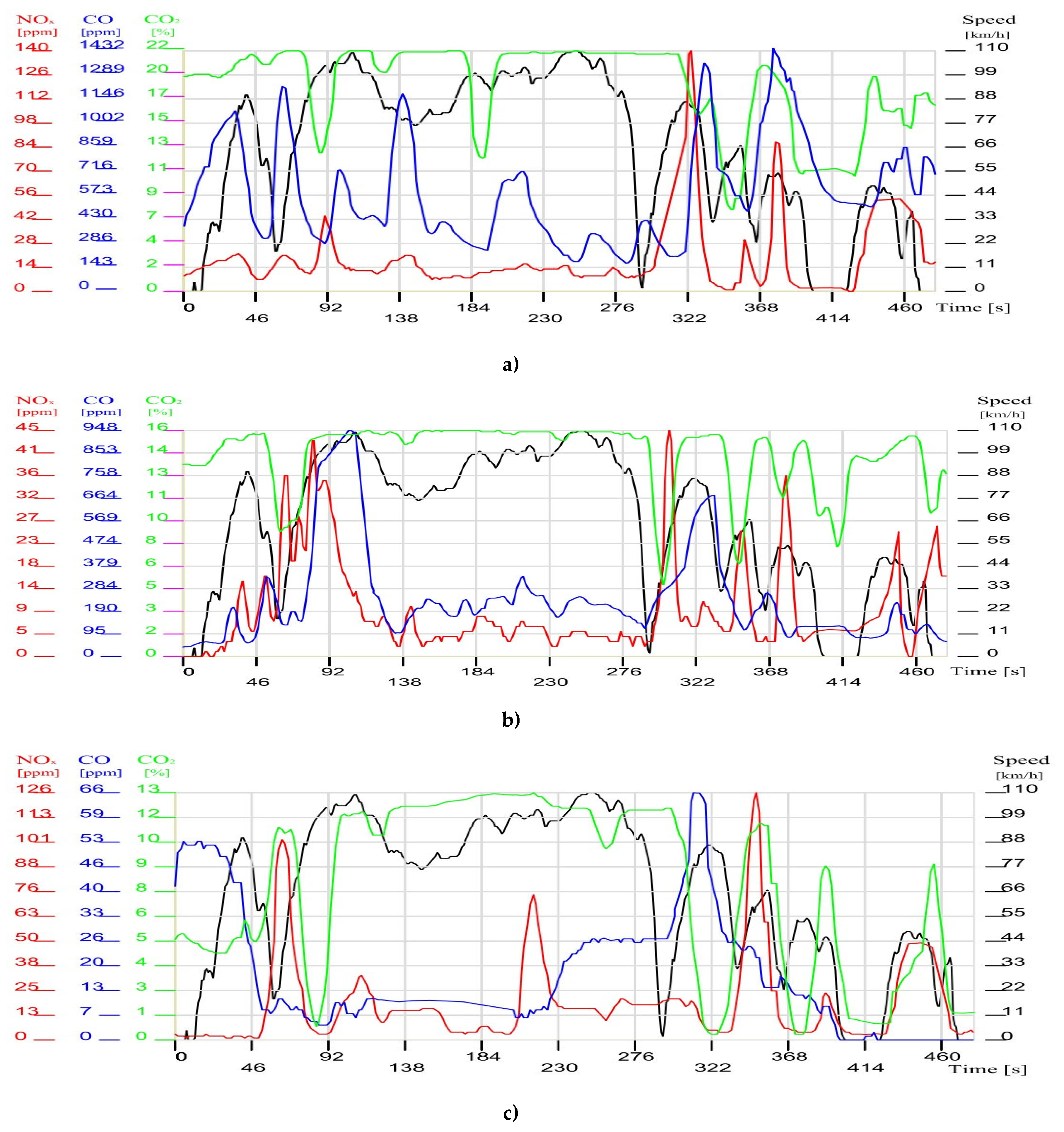
The analysis of the experimental results obtained on the dynamometric bench following the completion of the real mixed (urban-extraurban) driving cycle (M-BV Cycle) highlights the evolution of emissions in correlation with the engine load imposed by the travel speed of the studied road vehicles (in this cycle the travel speed was varied from 0 to 110 [km/h], (Figure 9).
The recorded instantaneous values of NOx emissions present developments related to the constructive and functional factors of the internal combustion engine.
The total NOx emissions of vehicles with spark ignition engines (SIE) show different values (Table 5 and Figure 11), namely: for vehicle 1, the total NOx value is 3867 [ppm] = 3867x103[μg/m3], and for vehicle 2, the total value is 6107 [ppm] = 6107x103 [μg/m3].
In the first gasoline vehicle (Bi-Turbo) instantaneous NOx emission values are recorded with smaller variations throughout the urban route with an increase during speed when the value of 138 [ppm] = 138x103 [μg/m3] was reached, in the case of vehicle 2 (engine with natural aspiration), a major dependence can be found between engine load and NOx emissions (NOx values increase depending on vehicle acceleration). This evolution can be explained by the evolution of the temperature in the engine cylinders which increases the formation rate of nitrogen oxides.
In the case of vehicles (Vehicle 3 and 4) with compression ignition (CIE) engines, it is found that the values of total NOx emissions have lower levels compared to the previous vehicles, thus vehicle 3 has a total emission of 1406 [ppm] = 1406 x103 [μg/m3] and vehicle 4 an emission of 3519 [ppm] = 3519 x103 [μg/m3], (Table 5 and Figure 11).
The instantaneous variations of NOx emissions fall between the values of 0–50 [ppm] = 0 -50x103 [μg/m3] with the exception of the single peak of 503 [ppm] = 503x103 [μg/m3] from the 65th second in which the load was total, 100 [%], (Figure 7c). And in this case, the explanation of the low values of NOx emissions can be mainly attributed to the reduced values of the gas temperatures in the engine cylinders and less due to the exhaust gas treatment systems.
In the case of the evolution of instantaneous CO emissions in vehicles with spark ignition engines, vehicles 1 and 2 (Figure 9a,b), several peaks can be found that can be explained by an imperfect combustion due to the operating regime transient at relatively low partial loads and under the conditions of a low thermal regime of the engines, the coolant during the test was in the range of 10 – 44 [0C]. In the case of vehicle 1 (SIE with bi-turbo system) the total emission per cycle is 8135 [ppm] = 8135 x103 [μg/m3] (Table 5), while in vehicle 2 (SIE, naturally aspirated -NA) the total CO emission is 3685 [ppm] = 3685 x103[μg/m3]. The explanation of this difference in CO emissions is given by the non-adaptation of the operating of the turbocharging system with the fuel system due to the low energy level of the exhaust gases of the engine of vehicle 1.
Analysis of real driving cycle CO emissions shows lower values for vehicles 3 and 4 which are equipped with turbocharged compression ignition engines. These values are: 2748 [ppm] = 2748x103 [μg/m3] in vehicle 3 and 1846 [ppm] = 1846 x103 [μg/m3] in vehicle 4, the explanation of the lower values for vehicles with spark ignition engines being the date of operation engine with lean air-fuel mixtures and more efficient gas treatment systems.
A very clear difference is highlighted by the peaks of carbon monoxide emissions that have low values of 124 [ppm] = 124 x103 [μg/m3] (Figure 10a) coming from diesel vehicles equipped with variable geometry gas turbines compared to those found in gasoline vehicles (over 1000 [ppm]= 1000 x103 [μg/m3] ( Figure 9a).
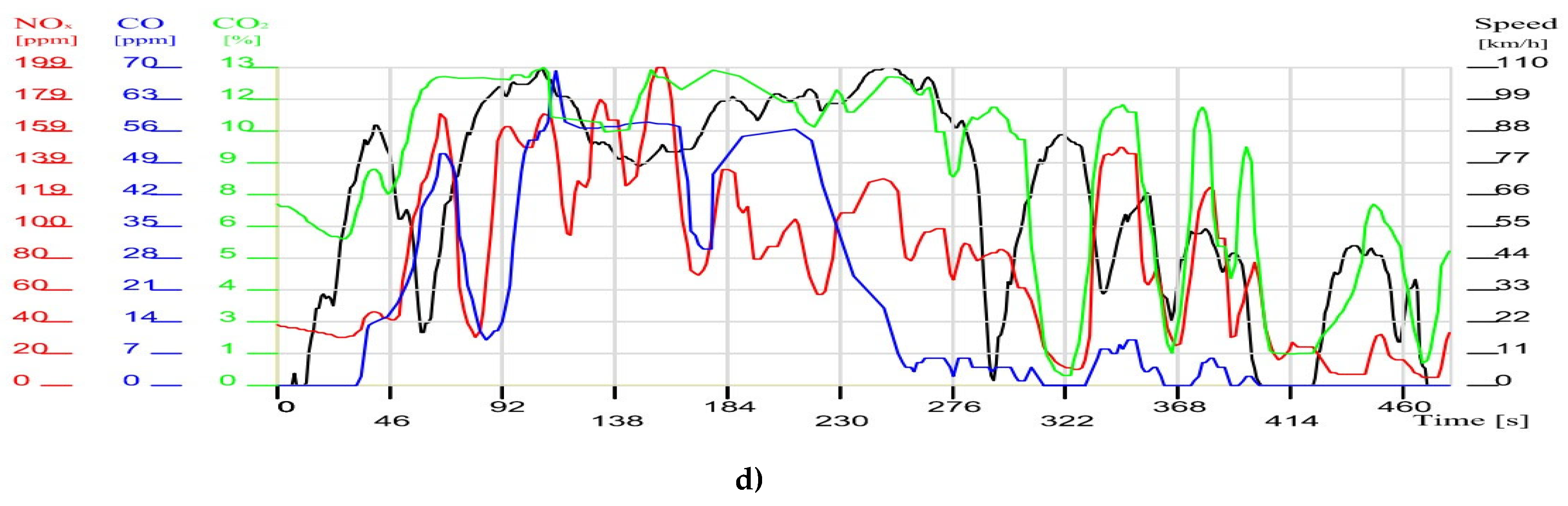
Figure 10.
Emissions variation diagram during the real mixed driving cycle (M-BV Cycle). a) Vehicle 3); b) Vehicle 4.
Figure 10.
Emissions variation diagram during the real mixed driving cycle (M-BV Cycle). a) Vehicle 3); b) Vehicle 4.
Instantaneous CO2 emission is the only component that fluctuates with vehicle speed in all four cases and closely tracks the fuel dose that gives the engine load and determines the vehicle’s speed. Total CO2 emissions during the real mixed driving cycle (M-BV Cycle) for vehicles with spark ignition engines reach values of: 18199[%] = 18199 x104 [μg/m3] in the case of vehicle 1 and of 20954 [%] = 20954 x104 [μg/m3] in the case of vehicle 2, in both cases the emission obviously remains dependent on the engine load. The high values can be explained by the homogeneous nature of the stoichiometric air-fuel mixture (λ=1) that is used in these engines.
The lower CO2 value recorded by vehicle 1 is explained by a more precise control of the fuel dose of this engine equipped with a bi-turbo supercharger system. Vehicles 3 and 4 equipped with compression ignition engines always run on lean air-fuel mixtures (λ>1) so that the total CO2 emission over the actual driving cycle is less than half of the previous spark ignition engine emissions of 8927 [%]= 8927 x104 [μg/m3] in vehicle 3 and of 8941[%]= 8941x104 [μg/m3] in vehicle 4, respectively.
4.3.2. Emissions on Extra-Urban Driving Cycle (E-BV Cycle)
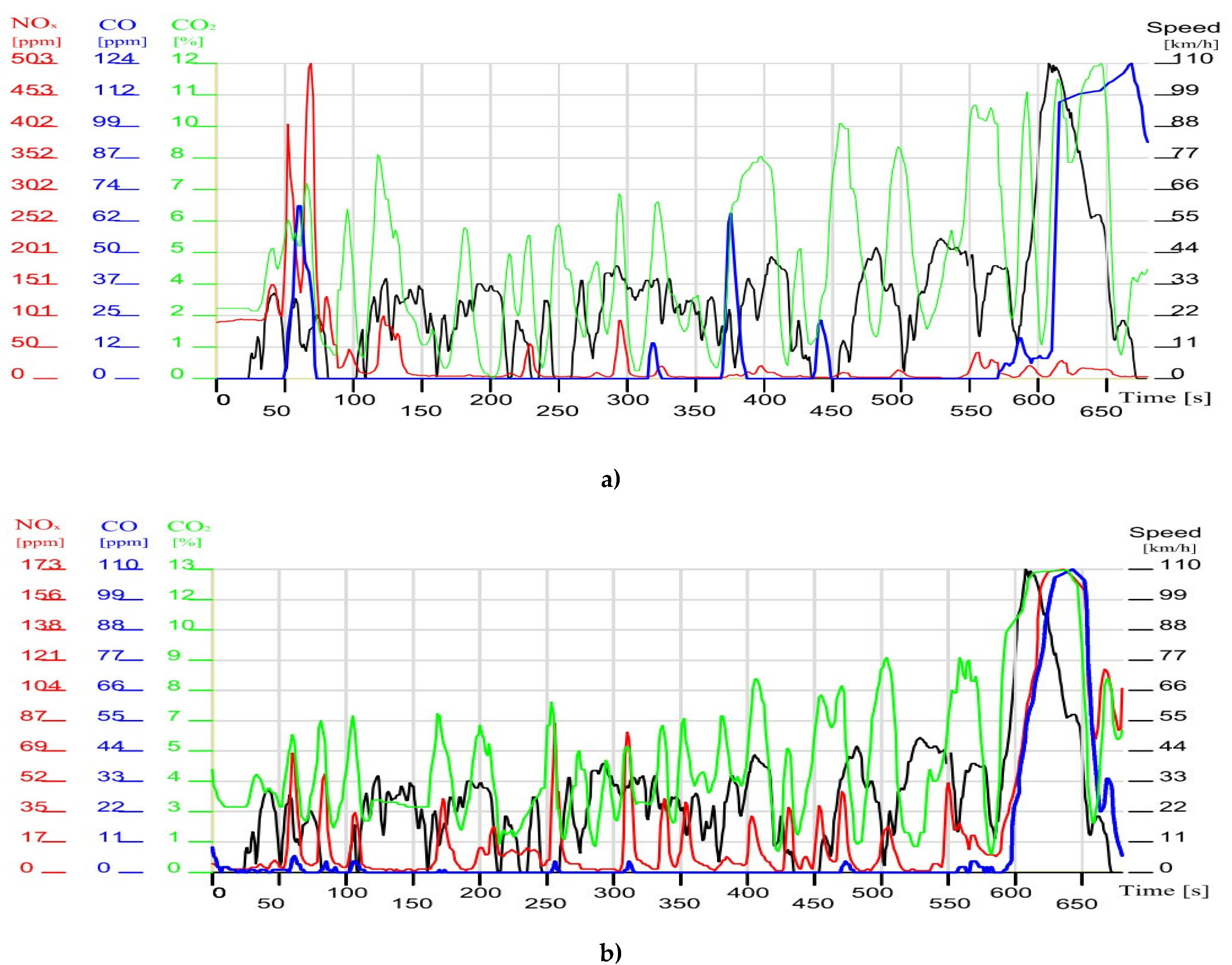
The following diagrams (Figure 11) present the experimental results obtained through tests on the studied vehicles using a real extra-urban driving cycle (E-BV Cycle) that describes a route outside the town, on road sections that allowed high and relativly constant speeds of cruise.
Thus, it can be determined if the analyzed pollutant emissions tend to decrease, stagnate or increase during the time when the speed of the travel is relatively constant, determining a quasi stable mode of operation of the engines of the studied vehicles. In the case of the real extra-urban driving cycle during the experiments, the NOx emissions showed total values per cycle with major differences depending on the type of vehicle engine and the type of NOx reduction equipment (Table 5 and Figure 12). Thus, in vehicles with spark ignition engines (Figure 11a,b), vehicle 2 with a naturally aspirated engine presented a total NOx emission per cycle of 5003 [ppm]= 5003 x103 [μg/m3] compared to vehicle 1 which is turbocharged with a system in two stages "bi-turbo" which had an emission of 3332 [ppm]= 3332 x103 [μg/m3], as both vehicles had similar gas treatment systems (TWC), the explanation of this emission difference is given by the higher gas temperatures in the engine cylinders of vehicle 2 due to of an efficient combustion process, temperatures that promoted the formation of NOx.
Total NOx emissions in the case of vehicles equipped with turbocharged diesel engines show higher value differences (Figure 11c,d), thus, vehicle 3 with a turbocharged diesel engine with a variable geometry turbine has an emission of 3619 [ppm]= 3619 x103 [μg/m3] and vehicle 4 with a turbocharged engine has an oemie approximately three times higher, in the amount of 9675 [ppm]= 9675 x103 [μg/m3]. This value difference has an explanation similar to the case of vehicles with spark ignition engines.
Instantaneous emissions during the tests with the four vehicles, except for the peaks recorded in the second gasoline vehicle (Figure 11b) where the values increase with acceleration (with increasing engine load).
Figure 11.
Emissions variation diagram during the real extra-urban driving cycle: a) Vehicle 1; b) Vehicle 2; c) Vehicle 3); d) Vehicle 4.
Figure 11.
Emissions variation diagram during the real extra-urban driving cycle: a) Vehicle 1; b) Vehicle 2; c) Vehicle 3); d) Vehicle 4.
It should be noted that the values of NOx emissions tend to decrease and stabilize when the vehicles maintain a constant speed (Figure 11a–c) even if the speeds are relatively high (over 100 km/h), less in the case of the fourth CIE vehicle where the oscillatory variation continues throughout the cycle.
The analysis of the total CO emissions per cycle resulting from vehicle testing using the real extraurban driving cycle "E-BV Cycle", shows that the level of these emissions in gasoline vehicles shows a major difference, as follows: vehicle 1 with a turbocharged engine has a total emission of CO of 9922 [ppm]= 9922 x103 [μg/m3], while vehicle 2 with a naturally aspirated (NA) engine has a total emission of 6112 [ppm]= 6112 x103 [μg/m3], (Table 5 and Figure 12 ).
Carbon monoxide is the result of an incomplete combustion of the fuel in the engine’s cylinders, so, because of an inefficient combustion process, these emission’s results of CO also confirms the results of the NOx emission, previously mentioned, but in fact, the construction of the engines, would have had opposiste values of the NOx emission CO emission. In the case of compression ignition engines, the values of total emissions per cycle are close, vehicle 3 with a total CO emission of 6203 [ppm] = 6203 x103 [μg/m3] and respectively of 6835 [ppm] = 6835 x103 [μg/m3] to vehicle 4. The transient regime imposed on the engine during the extra-urban cycle causes larger or smaller fluctuations in the CO emission depending on how the combustion in the engine is influenced (Figure 11a–d).
Table 5.
Driving cycle emissions values of tested vehicles.
| The Mixed Cycle (”M-BV Cycle”) | Extra-urban cycle (”E-BV Cycle”) | |||||
|---|---|---|---|---|---|---|
| NOx (x103) [μg/m3] |
CO (x103) [μg/m3] |
CO2 (x104) [μg/m3] |
NOx (x103) [μg/m3] |
CO (x103) [μg/m3] |
CO2 (x104) [μg/m3] |
|
| Vehicle 1 | 3867 | 8135 | 18199 | 3332 | 9922 | 20437 |
| Vehicle 2 | 6107 | 3685 | 20954 | 5003 | 6112 | 21306 |
| Vehicle 3 | 1406 | 2748 | 8927 | 3619 | 6203 | 14704 |
| Vehicle 4 | 3519 | 1846 | 8941 | 9675 | 6835 | 16195 |
Note: 1[ppm] = 103[μg/m3]; 1[ %] = 104[μg/m3].
Figure 12.
Diagram of total emissions at the end of the proposed cycles.
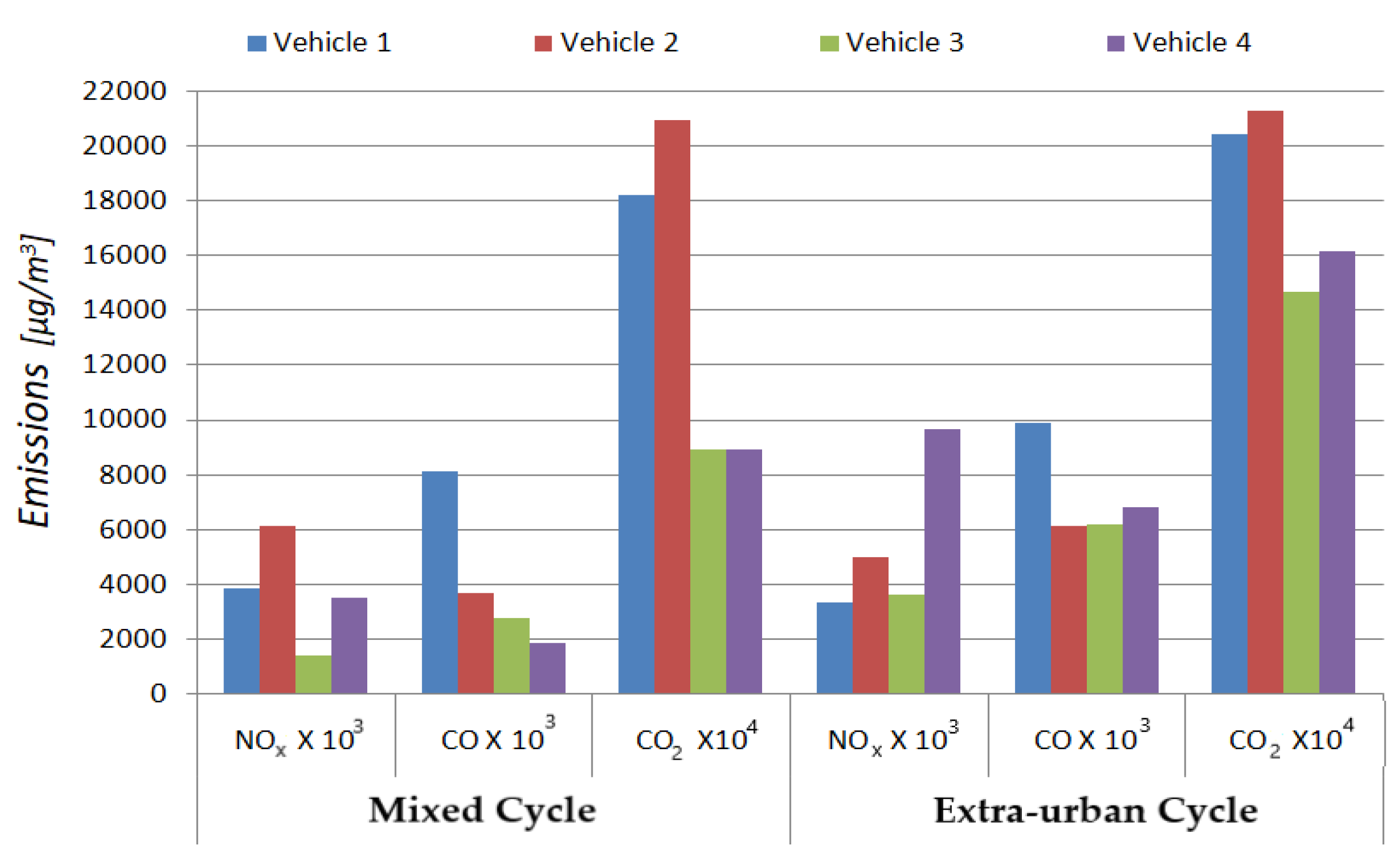
The total CO2 emissions during the "E-BV Cycle" extra-urban cycle vary depending on the type of engine,e.g., higher for spark ignition engines (SIE) that use stoichiometric air-fuel mixtures and lower for compression ignition engines (CIE) which always uses lean fuel air mixtures (Table 5 and Figure 12).
It should be noted that vehicle 1 on turbocharged gasoline has a total CO2 emission of 20437 [%]= 20437 x104 [μg/m3] lower than vehicle 2 (SIE-NA) which is of 21396 [%] = 21396 x104 [μg/m3], this evolution can be explained that in vehicle 1, part of the fuel was subjected to incomplete combustion turning into carbon monoxide (CO) emission.
In the case of vehicles 3 and 4 with compression ignition engines, the level of total CO2 emission per cycle is lower, being of 14703[%]= 14703 x104[μg/m3] in the case of vehicle 3, and the total CO2 emission in the vehicle 4 being of 16195 [%] = 16195x104 [μg/m3].
The variations in the instantaneous CO2 emissions recorded for the four studied vehicles are much lower due to the smaller influence of the load variations on the combustion processes in the vehicle engines.
4.3.3. Fuel Consumption Results
The records regarding the fuel consumption of the four vehicles during the real mixed cycle "M-BV Cycle" are presented in Figure 13 and the total consumption per cycle in Table 6 and Figure 15.
The instantaneous consumption diagrams of the two vehicles with spark-ignition engines are shown in Figure 13a, where it is noted that the variation of instantaneous consumption is similar, but in the case of vehicle 2 with a naturally aspirated engine, the consumption peaks sound more vigorous, so it shows a total fuel consumption per cycle of 776 [g] higher than vehicle 1 which 669 [g] these quantities divided by the duration of the cycle give the values of the average hourly consumption per cycle 5.39 [l/h] (vehicle 2) respectively 4.51 [l /h] (vehicle 1) this difference being 16.33 [%].
The evolution of the instantaneous fuel consumption of vehicles with compression ignition engines are shown in Figure 13b, the magnitude of fuel consumption peaks in vehicle 3 with an engine equipped with a variable geometry turbocharger is lower than vehicle 4 with a turbocharged engine, similarly to vehicle 3, where there is a lower fuel requirement in this transitory mode. This is also demonstrated by the total fuel consumption per cycle, vehicle 3 is of 538 [g] and relative to the cycle time the average hourly consumption per cycle is of 3.73 [l/h], in the case of vehicle 4 the total consumption is of 566 [g] which gives an average hourly consumption per cycle of 3.92 [l/h], the difference between the consumptions of this engine is small, that is, (5.20 [%]).
If we compare the lowest fuel consumption of gasoline engines with that given by the diesel engine, a difference of 17.10 [%] is obtained.
The research results regarding the instantaneous fuel consumption and the total fuel consumption per cycle when running on the dynamometric bench and of the four vehicles selected for the tests, following the extra-urban cycle ("E-BV Cycle") are presented in Figure 14, Figure 15 and the Table 6. If we compare the results regarding the instantaneous consumption of vehicles equipped with gasoline engines, it is found that the fuel consumption peaks in vehicle 1 equipped with a turbocharger (bi-turbo) are higher than in the case of vehicle 2 with a naturally aspirated engine (Figure 13a), so the level of total fuel consumption per cycle for vehicle 1 is of 765 [g] which gives an average hourly consumption per cycle of 7.64 [l/h], and for vehicle 2 of 609 [g], the average hourly consumption per cycle being of 6.08 [l/h], the consumption difference is 25.62 [%].
Figure 14.
Fuel consumption variation diagram – extra-urban driving cycle (”E-BV Cycle”). a) Vehicle 1 and vehicle 2; b) Vehicle 3 and vehicle 4.
Figure 14.
Fuel consumption variation diagram – extra-urban driving cycle (”E-BV Cycle”). a) Vehicle 1 and vehicle 2; b) Vehicle 3 and vehicle 4.
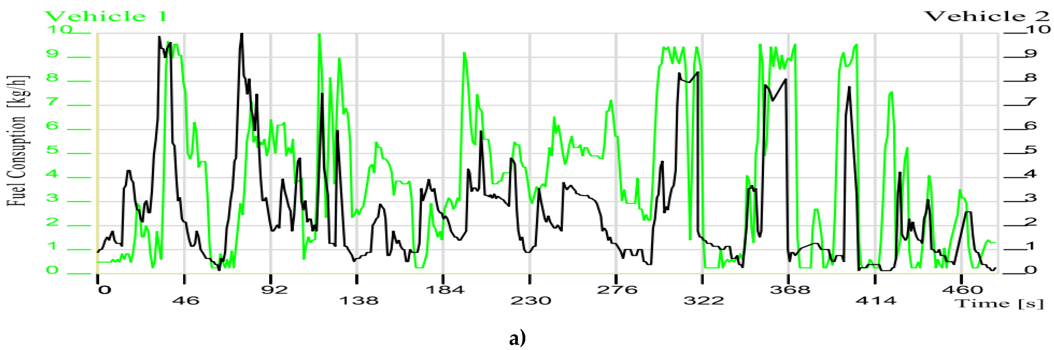
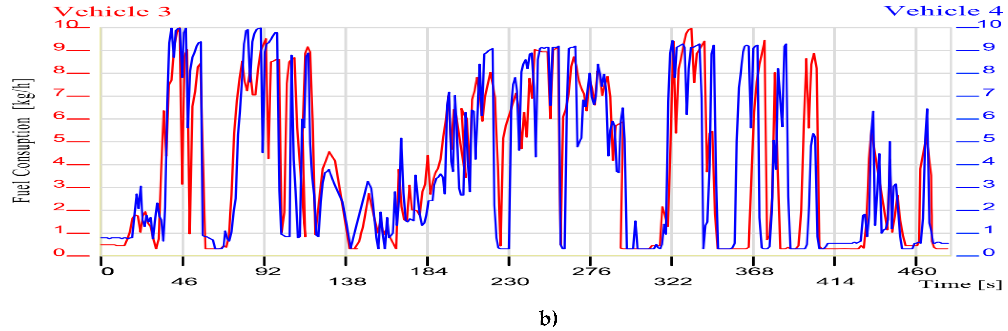
Table 6.
Total fuel consumption during mixed and extra-urban cycles.
| Cycle | Mixed Cycle (”M - BV Cycle”) | Extra-urban Cycle (”E-BV Cycle”) | ||||
|---|---|---|---|---|---|---|
| M.U. | [g] | [kg/h] | [l/h] | [g] | [kg/h] | [l/h] |
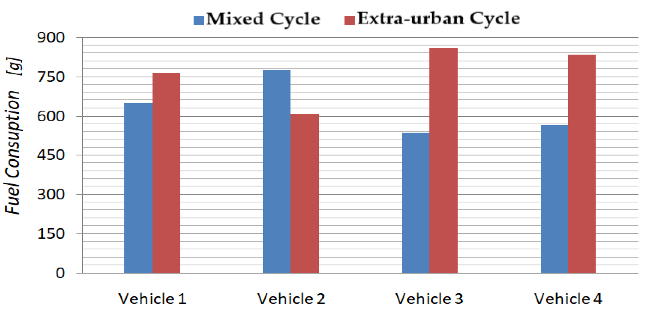
| Vehicle 1 | 649 | 3.38 | 4.51 | 765 | 5.73 | 7.64 |
| Vehicle 2 | 776 | 4.04 | 5.39 | 609 | 4.56 | 6.08 |
| Vehicle 3 | 538 | 2,80 | 3.73 | 860 | 6.44 | 8.59 |
| Vehicle 4 | 566 | 2,94 | 3.92 | 834 | 6.24 | 8.32 |
Figure 15.
Total fuel consumption during mixed (”M - BV Cycle”) and extra-urban cycles (”E - BV Cycle”).
Figure 15.
Total fuel consumption during mixed (”M - BV Cycle”) and extra-urban cycles (”E - BV Cycle”).
The analysis of the variation curves of the instantaneous fuel consumptions in the case of vehicle 3 and vehicle 4, shows small differences, so the levels of total fuel consumptions have close values, 860 [g] for vehicle 3 and 834 [g] for vehicle 4, these consumptions related to the duration of the extra-urban cycle will give the average hourly consumption values per cycle of 38.59 [l/h] and of 8.32 [l/h] respectively, the difference between these values being of 3.11 [%].
5. Discussion
The experimental research carried out had as a main purpose the creation of an effective work tool, in this case, the real driving cycle to be used to assess the participation of light vehicle emissions in air pollution in the urban area. At the same time, the results of this experimental research on emissions and fuel consumption, in urban and extra-urban traffic conditions, highlights the main parameters of influence related to: the characteristics of the vehicles’ propulsion system; the particularities of the road infrastructure; drivers’ driving style of vehicles and the weather factors.
5.1. Selecting Routes and Modelled Test Driving Cycles
The selection of routes to generate real driving cycles requires a special attention, mainly because the specific characteristics of urban transport must be taken into account. These specific features are as follows:
- -
- Transport is carried out in limited road spaces, which have fixed dimensions; it is not possible to store unused road capacity for use over periods of higher demand.
- -
- "Derived" transport demand, in this case, trips are not made for the sake of the desire to travel, but are generated by the need to move to places where different types of activities are carried out, such as, work, shopping, studies, recreation, relaxation etc., in different locations;
- -
- Transport demand is highly variable and shows peak periods that concentrate a large number of journeys in a short period of time due to the desire to make the best use of the time available for those various activities.
Due to these characteristics, congestion occurs in different points of the road infrastructure, with all its negative consequences, the increase in emissions, high fuel consumption and time consumption by extending the duration of the trip, this congestion having negative effects on the quality of life.
In order to establish the routes for carrying out the research, a traffic study was previously carried out in order to establish the preferences of drivers’ motor vehicle in choosing the way to cover the distance between the departure point and the arrival point.
Once the itinerary of the route established, the model of the mixed driving cycle has been finalized. It is composed of road segments from the old city, through the new neighborhoods and connecting segments with various destinations, and after the road route intended to model the extra-urban driving cycle has been chosen, representing a part of approx. 30% of the bypass belt of the city of Brasov, the hourly interval for carrying out the research was established, being the traffic peak. In order to determine the daily influence of traffic parameters on emissions and energy consumption, the days when the attempts were repeated in the same time interval are set.
The influence of the driver’s characteristics was eliminated as there was the same person for all the tests performed on the test routes.
The data obtained when travelling the routes for the two proposed cycles (the mixed cycle and the extra urban cycle) allowed the modelling of four sets of real driving cycles with different characteristics (Table 4) depending on the day on which the data were recorded.
Based on the analysis of these characteristics, the set of cycles (the mixed cycle and the extra-urban cycle) was selected and was used for the research of the four vehicles in order to determine their emissions and fuel consumption.
5.2. Vehicle Emissions and Fuel Consumption During Real Driving Cycles
The resulting emission values are those measured on the tail pipe and depend on the influence of the traffic parameters that determine the operational factors of the propulsion system. The usefulness of these obtained data is given by the possibility of being analyzed later on by using pollutant dispersion models to determine the participation of this road traffic in air pollution in urban areas. Dispersion models use the laws of fluid dynamics and can be represented by a set of equations with partial derivatives: fluid motion equations, mass and energy conservation equations, diffusion equation.
It should be stated that the experimental research, both on the selected streets and on the dynamometric stand following the adopted cycles were carried out in the cold season, the beginning of spring time. From the analyzes of the data collected during the experimental research both on the real route and on the dynamometric stand following the selected cycles, it was found that the engines of the propulsion systems of the tested vehicles operated at thermal regimes (Table 7) much lower than their normal operating values, of 90 - 105[0C].
Low engine’s temperature regimes result in low operating efficiencies and higher engine’s emissions due to increased frictional losses and inefficient combustion processes. The main factor responsible for this is the temperature of the cylinder liner which determines the temperature level of the coolant; in fact, it influences the temperature of the lubricant and therefore the friction losses, especially during the warm-up. When it is a low temperature of the lubricant, about 20 [°C], it is estimated that frictional losses can be up to 2.5 times higher than in normal heating conditions.
The convergent effects of engines’ operation of these vehicles at thermal regimes below the normal limit worsen the combustion processes and cause an increase in mechanical losses with a reduction in operating efficiencies, together with the dynamic regime at partial loads imposed by the configuration of the real test driving cycle, all these effects cause a dramatic increase in consumption average fuel per cycle (Table 8.)
This increase is by 2 - 3 times higher than that indicated by the manufacturers of these vehicles. Under these circumstances, it would be necessary to limit urban trips in cold weather, as the normal operating temperatures of the engines cannot be reached and the negative effects are numerous, emissions and increased consumption data, as well.
The vehicles selected for the research were equipped with after-treatment systems, such as: three-way catalytic converters (TWC) for gasoline engines, and a diesel oxidation catalytic converter (DOC) system, together with selective catalytic reduction converters ( SCR) and diesel particulate filters (DPF) for compression ignition engines. All of these after-treatment systems are catalytic converters and their functionality deteriorates at low temperature levels, as, during cold start and engine warm-up phases to normal operating temperature. In fact, catalysts convert pollutant emissions only when their temperature reaches certain thresholds, i.e. the so-called light-off temperature, which for most TWCs is normally around 250–300[°C]. Because of this, high levels of exhaust emissions are released into the atmosphere during the time when the exhaust gas temperature is low, during the cold start and/or engine warm-up phases, when the catalyst is not on fully operational.
Therefore, the high values of the emissions can be explained, for example, the measured CO emissions per mixed driving cycle of 8135 [ppm] = 8135 x103[μg/m3] and 3685 [ppm] = 3685 x103[μg/m3] for gasoline engines, and of 2748 [ppm] = 2748x103[μg/m3] and of 1846[ppm] = 1846 x103[μg/m3] for diesel engines on conditions of cold start and operation at low thermal regimes, emissions being caused by combustion the precariousness of the fuel-air mixture and the low efficiency of the catalytic systems for treating the burnt gases.
6. Conclusions
The research carried out and presented in this paper aimed at the development of real driving cycles to be implemented on the dynamometric bench to make it possible to test different vehicles on the same traffic conditions for a more precise determination of emissions and fuel consumption values.
Achieving this goal has required a careful study of the main traffic flows in order to correctly select the route that serves to develop the actual driving cycle. The selected route took into account the influences that could be generated by elements such as: road class and location, traffic density, the number of intersections, the number of pedestrian crossings and their traffic density and limiting speed restrictions on emissions and fuel consumption.
In order to detect the influences given by the various elements, the data necessary for modelling the real driving cycles were collected on four different days in the same time interval, resulting in a set of four mixed cycles and four extra-urban cycles. These cycles had different characteristics and the parameters varied within perceptible limits (e.g. the duration of the cycle varied within a range of 31.06 [%], and the average speed of the cycle with stops varied between 28.10 [km/h] and 36.82 [km/ h], the range being 31.03[% ]). So, an analysis of some possible development scenarios was needed to lead to the decision of choosing the cycle to be used for vehicle testing.
The development of these real driving cycles highlighted the need to introduce an intelligent traffic management system to eliminate the uncertainty factors that appeared due to the existing system, and this system would be able to eliminate part of the transient regimes due in particular to speed reductions in order to ensure safe traffic.
The choice of vehicles for the tests was a challenge because they had to be representative for the category of vehicles referred to in the analyzes regarding the contribution of emissions released into the environment. The vehicles selected to be tested corresponded to the EURO 6 (2014) pollution standard because the fleet of light vehicles was renewed due to some government programs and these vehicles were the majority part.
The testing of the selected vehicles on the dynamometric bench after the actual driving cycle implemented showed differences in instantaneous emissions and total emissions per cycle, influenced by the particularities of the vehicle’s propulsion system and the operating regime given by the cycle parameters. The resulting values confirmed a lower participation of these vehicles in the pollutant levels recorded by the air quality monitoring stations.
Fuel consumption had a similar trend to that of emissions, being influenced by the same factors.
Author Contributions
Conceptualization, N.C. and C.C.; methodology, N.C. and C.C.; software, N.C.; validation, C.C.; formal analysis, P.V.; investigation, N.C. and C.C.; resources, C.C.; data duration, C.C. and P.V.; writing—original draft preparation, N.C. and C.C.; writing—review and editing, C.C. and P.V.; visualization, N.C. and C.C.; supervision, C.C. and P.V.; project administration, C.C.; funding acquisition, N.C., C.C. and P.V. All authors have read and agreed to the published version of the manuscript.
Funding
This funding was supported by Transilvania University Brasov, 500036 Brasov, Romania.
Institutional Review Board Statement
Not applicable.
Informed Consent Statement
Not applicable.
Data Availability Statement
The raw data supporting the conclusions of this article will be made available by the authors on request.
Acknowledgments
We thank Professor Dinu Covaciu (Department of Motor Vehicles and Transport) for all the support provided throughout the research.
Conflicts of Interest
The authors declare not conflict of interest.
References
- Commission Regulation (EU) 2017/1151 of 1 June 2017 supplementing Regulation (EC) No 715/2007 of the European Parliament and of the Council on type-approval of motor vehicles with respect to emissions from light passenger and commercial vehicles (Euro 5 and Euro 6). Available online: http://data.europa.eu/eli/reg/2017/1151/oj.
- Liqiang, H.; Jingnan, H.; Shaojun, Z.; Ye, W.; Rencheng, Z.; Lei, Z.; Xiaofeng, B.; Yitu, L.; Sheng, S. The impact from the direct injection and multi-port fuel injection technologies for gasoline vehicles on solid particle number and black carbon emissions. Applied Energy 2018, 226, 819–826. [Google Scholar] [CrossRef]
- Dernotte, J.; Najt, P.; and Durrett, R. Downsized-Boosted Gasoline Engine with Exhaust Compound and Dilute Advanced Combustion. SAE Int. J. Adv. & Curr. Prac. in Mobility 2020, 2, 2665–2680. [Google Scholar] [CrossRef]
- Duan, X.; Liu, J.; Tan, Y.; Luo, B.; Guo, G. Influence of single injection and two-stagnation injection strategy on thermodynamic process and performance of a turbocharged direct-injection spark-ignition engine fuelled with ethanol and gasoline blend. Applied Energy 2018, 228, 942–953. [Google Scholar] [CrossRef]
- Guardiola, C.; Martín, J.; Pla, B.; Bares, P. Cycle by cycle NOx model for diesel engine control. Applied Thermal Engineering 2017, 110, 1011–1020. [Google Scholar] [CrossRef]
- Überall, A.; Otte, R.; Eilts, P.; Krahl, J. A literature research about particle emissions from engines with direct gasoline injection and the potential to reduce these emissions. Fuel 2015, 147, 203–207. [Google Scholar] [CrossRef]
- Ghanbari, M.; Najafi, G.; Ghobadian, B.; Yusaf, T. Performance and emission characteristics of a CI engine using nano particles additives in biodiesel-diesel blends and modelling with GP approach. Fuel 2017, 202, pp. 699–716, ISSN: 0016. [Google Scholar] [CrossRef]
- Hergueta, C.; Bogarra, M.; Tsolakis, A.; Essa, K.; Herreros, J.M. Butanol-gasoline blend and exhaust gas recirculation, impact on GDI engine emissions. Fuel 2017, 208, 662–672. [Google Scholar] [CrossRef]
- Constantine, D.R.; Athanasios, M.D.; Evangelos, G.G.; Dimitrios, C.R. Investigating the emissions during acceleration of a turbocharged diesel engine operating with bio-diesel or n-butanol diesel fuel blends. Energy 2010, 35, 5173–5184. [Google Scholar] [CrossRef]
- Yinhui, W.; Rong, Z.; Yanhong, Q.; Jianfei, P.; Mengren, L.; Jianrong, L. The impact of fuel compositions on the particulate emissions of direct injection gasoline engine. Fuel 2016, 166, 543–552. [Google Scholar] [CrossRef]
- Szpica, D. Coefficient of Engine Flexibility as a Basis for the Assessment of Vehicle Tractive Performance. Chinese Journal of Mechanical Engineering 2019, 39, https:doi.org/10.1186/s10033–019. [Google Scholar] [CrossRef]
- Liu, J.; Dumitrescu, C. Flame development analysis in a optical engine converted to spark ignition natural gas operation. Applied Energy 2018, 230, 1205–1217. [Google Scholar] [CrossRef]
- Chen, L.F.; Liang, Z.R.; Zhang, X.; Shuai, S.J. Characterizing particulate matter emissions from GDI and PFI vehicles under transient cold-startand cold start condition. Fuel 2017, 189, 131–140. [Google Scholar] [CrossRef]
- Tarulescu, S.; Cofaru, C.; Tarulescu, R. Cold Engine’s Operating Regime Influence over the Exhaust Emissions. Applied Mechanics and Materials 2016, 822, 219–223. [Google Scholar] [CrossRef]
- Liye, B.; Jihua, W.; Lihui, S.; Haijun, C. Exhaust Gas After-Treatment Systems for Gasoline and Diesel Vehicles. International Journal of Automotive Manufacturing and Materials 2022, 1. [Google Scholar]
- Uditha, G.; Loshaka, P.; Saman, B. Developing a General Methodology for Driving Cycle Construction: Comparison of Various Established Driving Cycles in the World to Propose a General Approach. Journal of Transportation Technologies 2015, 5(4). [Google Scholar] [CrossRef]
- Tong, H.Y.; Hung, W.T. On-Road Motor Vehicle Emissions and Fuel Consumption in Urban Driving Conditions. Journal of the Air & Waste Management Association 2011, 50, 543–554, ISSN 1047-3289. [Google Scholar]
- Kęska, A. The Actual Toxicity of Engine Exhaust Gases Emitted from Vehicles: The Development and Perspectives of Biological and Chemical Measurement Methods. ACS Omega. 2023, Jul 18; Vol.8, Issue 28, pp 24718–24726. [CrossRef]
- Principles of calculating results by the Madur Gas Analysers, Madur Electronics, 07/2007. Available online: www.madur.com.
- User’s manual for CAP 3201, EMISSION STATION, Capelec Ergonomics Efficency Simplicity. Available online: www.capelec.fr.
- Andrew, R.; Richard, B.; Shipway, P. Internal combustion engine cold-start efficiency: A review of the problem, causes and potential solutions. Energy Conversion and Management 2014, 82, 327–350. [Google Scholar] [CrossRef]
- Evangelos, G.; Giakoumis, T.; George, T. Analysis of the Effect of Vehicle, Driving and Road Parameters on the Transient Performance and Emissions of a Turbocharged Truck. Energies 2018, 11, 295. [Google Scholar] [CrossRef]
- Bahmankhah, B.; Macedo, E.; Fernandes, P.; Coelho, M. Micro driving behaviour in different roundabout layouts: Pollutant emissions, vehicular jerk, and traffic conflicts analysis. Transportation Research Procedia 2022, 62, 501–508. [Google Scholar] [CrossRef]
- Cofaru, C. Autovehiculul si poluarea mediului:evaluare si control. Editura Universitatii “Transilvania Brasov”, 2015 ISBN 978-606-19-0666-6.
- Guanfeng, Y.; Mingnian, W.; Tao, Y. Pengcheng Qin Effects of traffic patterns on vehicle pollutant emission factors in road tunnels. Tunnelling and Underground, Space Technology 2022, 130. [Google Scholar] [CrossRef]
- Samuel, A.; Charles, A.; Gift, D.; Atinuke, O. The Impact of Vehicle Engine Characteristics on Vehicle Exhaust Emissions for Transport Modes in Lagos City. Urban, Planning and Transport Research. Open Access Journal 2024, 12. [Google Scholar] [CrossRef]
- Ibrahim, R.; Mahmoud, E.; Khaled, Z.; Fabio, T.; Ibrahim, S. Effect of Road, Environment, Driver, and Traffic Characteristics on Vehicle Emissions in Egypt. International Journal of Civil Engineering 2022, 20, 1261–1276. [Google Scholar] [CrossRef]
- Luc, I.; Steven, B.; Ronghui, L. Modelling instantaneous traffic emission and the influence of traffic speed limits. Science of the Total Environment 2006, 371, 270–285. [Google Scholar] [CrossRef]
- Ali, I.; Hamid, A. Investigating the Effect of Traffic Flow on Pollution, Noise for Urban Road Network. IOP Conf. Ser.: Earth Environ. Sci. 2022, 961, 012067. [Google Scholar] [CrossRef]
- Suresh, P.; Sharad, G.; Aloke, G. Evaluating effects of traffic and vehicle characteristics on vehicular emissions near traffic intersections. Transportation Research Part D:Transport and Environment 2013, 23, 114. [Google Scholar] [CrossRef]
- Šarić, A.; Sulejmanović, S.; Albinović, S.; Pozder, M.; Ljevo, Ž. The Role of Intersection Geometry in Urban Air Pollution Management Air Pollution Management. Sustainability 2023, 15, 5234. [Google Scholar] [CrossRef]
- Dragomir, M.; Cuzmin, C.; Șerban, C.; Munteniță, C. The impact of road transport emissions on air quality in Brăila, Romania. PESD 2021, Volume 15.
- Vladimir, S.; Aleksandr, I.; Slobodi, M. Studying the Relationship between the Traffic Flow Structure, the Traffic Capacity of Intersections, and Vehicle-Related Emissions. Mathematics 2023, 11, 3591. [Google Scholar] [CrossRef]
- Katarzyna, B.; Zdzisław, C.; Krystian, S.; Magdalena, Z. The Influence of the Properties of Vehicles Traffic on the Total Pollutant Emission. Zeszyty Naukowe Instytutu Pojazdów, Instytut Pojazdów Politechniki Warszawskiej, Proceedings of the Institute of Vehicles 2017, Volume 1, pp. 89–102. Available online: https://repo.pw.edu.pl/info/article.
- Fangfang, Z.; Jie, L.; Henk, Z.; Chao, L. Influence of driver characteristics on emissions and fuel consumption. Transportation Research Procedia 2017, 27, 624–631. [Google Scholar] [CrossRef]
- Papageorgiou, N.; Demetris, D.; Elena, T.; Athanasios, M. Analyzing the Requirements for Smart Pedestrian Applications: Findings from Nicosia, Cyprus. Smart Cities 2024, 7, 1950–1970. [Google Scholar] [CrossRef]
- Available online: https://ec.europa.eu/eurostat/web/products-eurostat-news/w/ddn-20230530-1.
- Available online: https://ec.europa.eu/eurostat/web/products-eurostat-news/w/ddn-20240117-1.
- Available online: https://www.statista.com/statistics/452238/europe-eu-28-number-of-cars-per-1000-inhabitants/.
- Available online: https://www.acea.auto/figure/per-capita-new-car-registrations-by-eu-country/.
- Available online: https://statzon.com/insights/e-mobility-europe-an-overview-of-europes-latest-electric-vehicles-data.
- Available online: https://ec.europa.eu/eurostat/statistics-explained/index.php?title=Transport_equipment_statistics.
- Available online: https://www.brasovcity.ro/filezone/mediu/planuriactiune/aer/Plan%20Integrat%20de%20Calitate%20a%20Aerului%20in%20Municipiul%20Brasov%202023-2027.pdf.
Figure 1.
Hourly maximum concentrations of NOx recorded at the air quality monitoring stations in the municipality of Brașov BV-1, BV-2, BV-3 and BV-5 over the period 2010–2022, (Data source: www.calitateaer.ro) [43]. Translated terms: Ani =Years; Valoare limită orara = Hourly limit value.
Figure 1.
Hourly maximum concentrations of NOx recorded at the air quality monitoring stations in the municipality of Brașov BV-1, BV-2, BV-3 and BV-5 over the period 2010–2022, (Data source: www.calitateaer.ro) [43]. Translated terms: Ani =Years; Valoare limită orara = Hourly limit value.
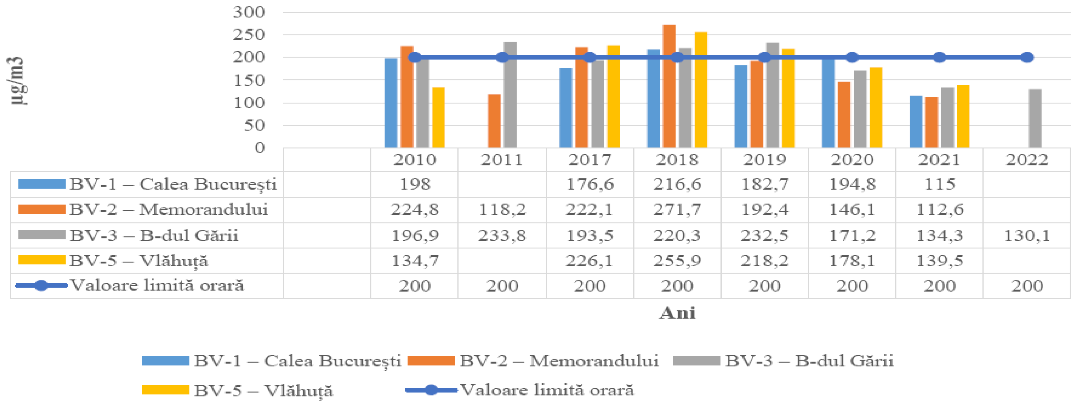
Figure 2.
General diagram of experimental research.
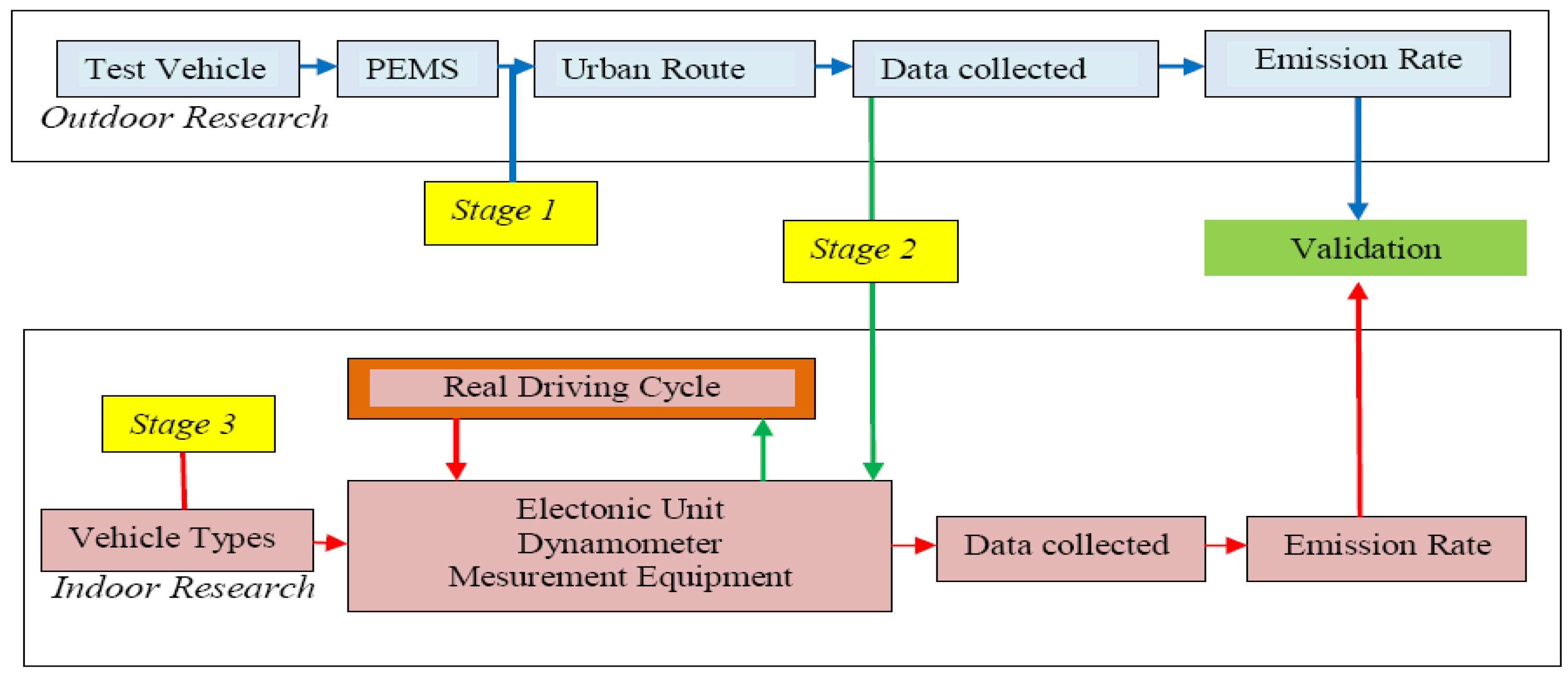
Figure 3.
Road routes selected for analysis: (a) Urban –extra-urban (mixed); (b) Extra- urban.
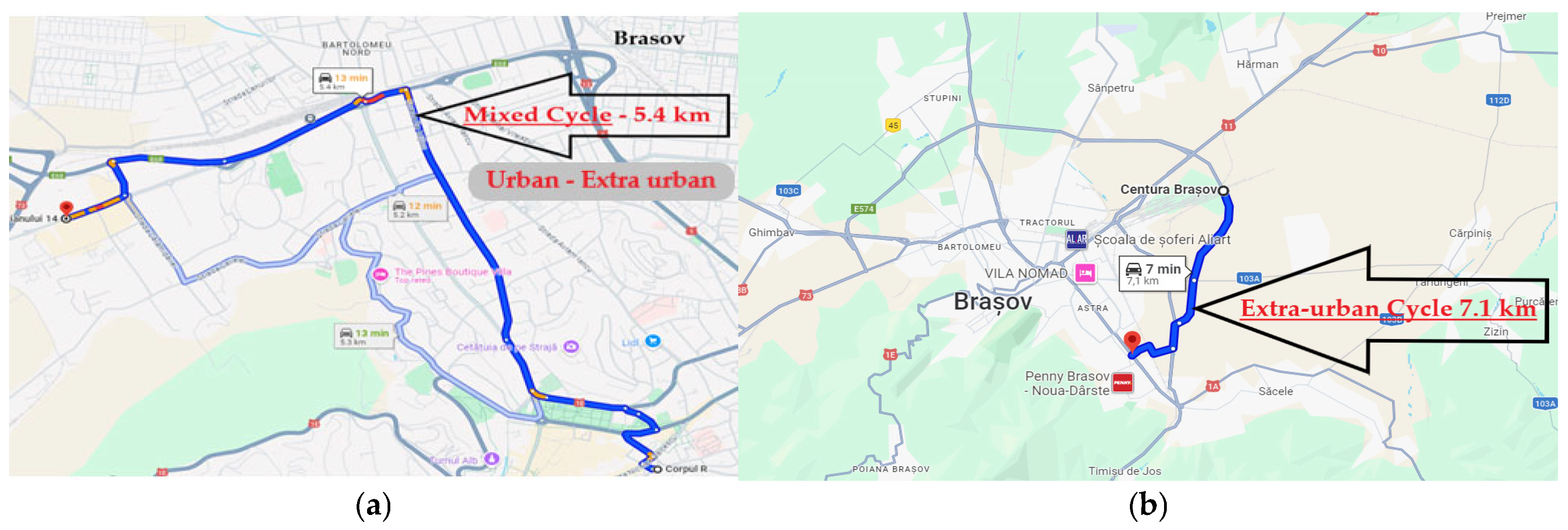
Figure 4.
View of the positioning of the fuel flow measurement system on the vehicle.
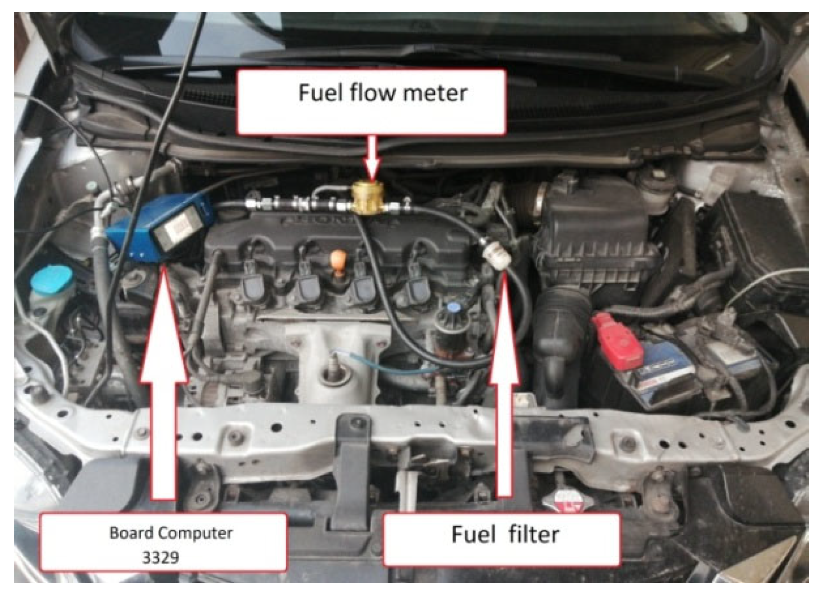
Figure 5.
Schematic of the on-board fuel flow measurement installation: a) SIE vehicles; b) Vehicles with Diesel engines.
Figure 5.
Schematic of the on-board fuel flow measurement installation: a) SIE vehicles; b) Vehicles with Diesel engines.
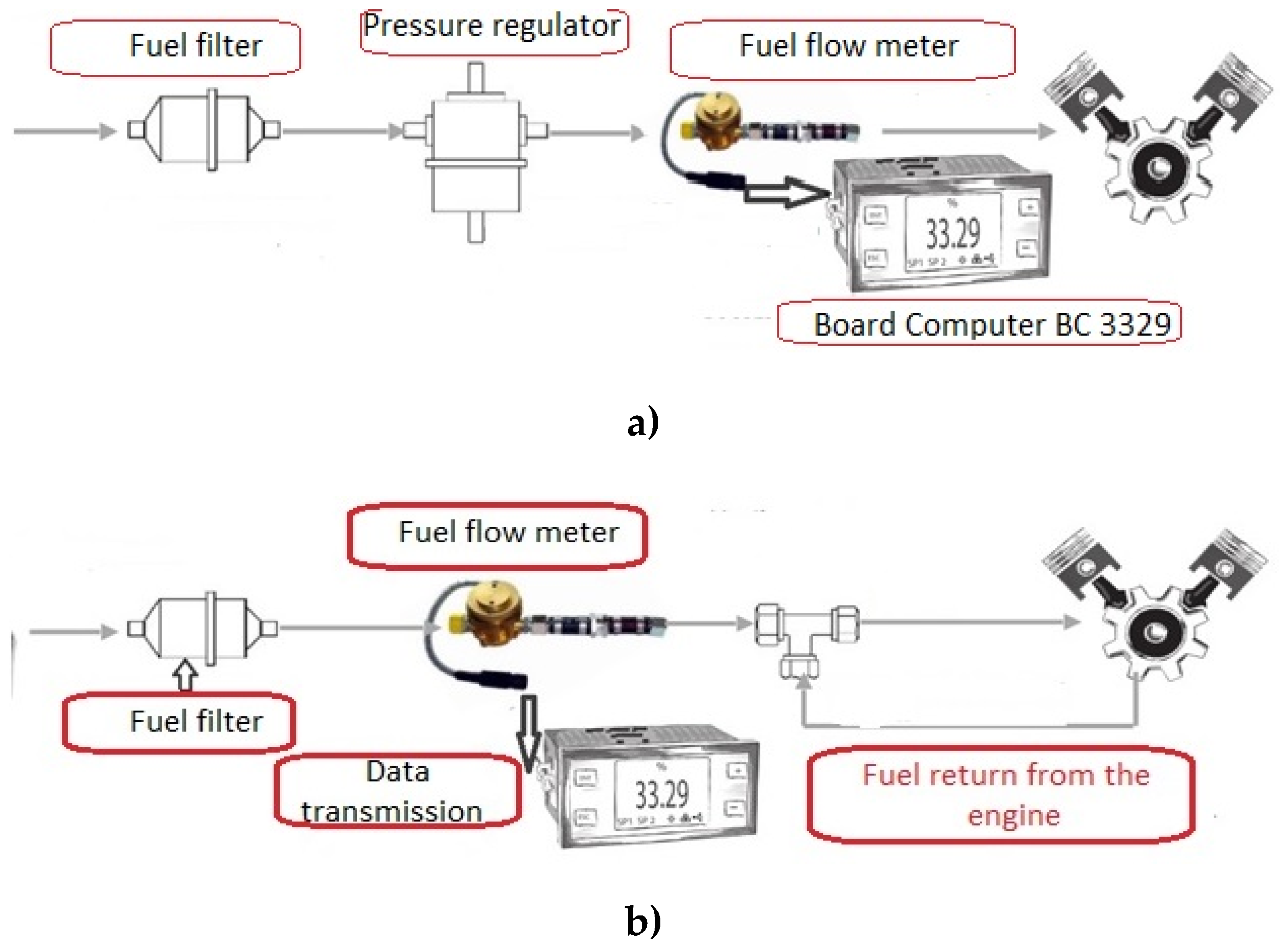
Figure 7.
The real driving test cycle.
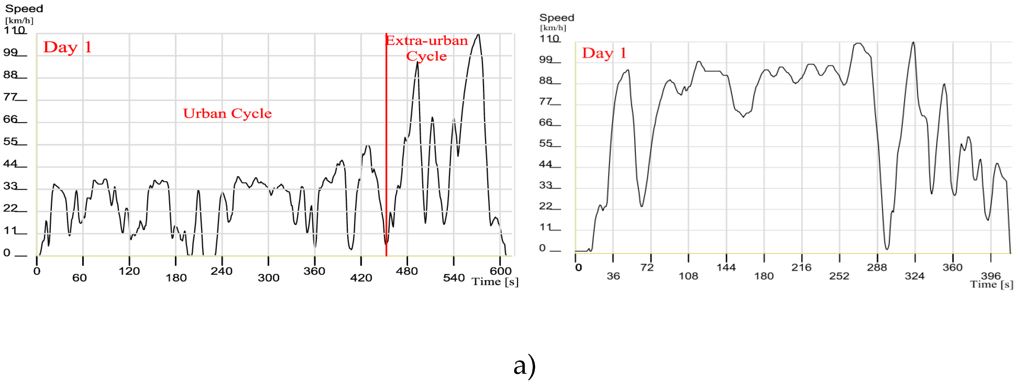
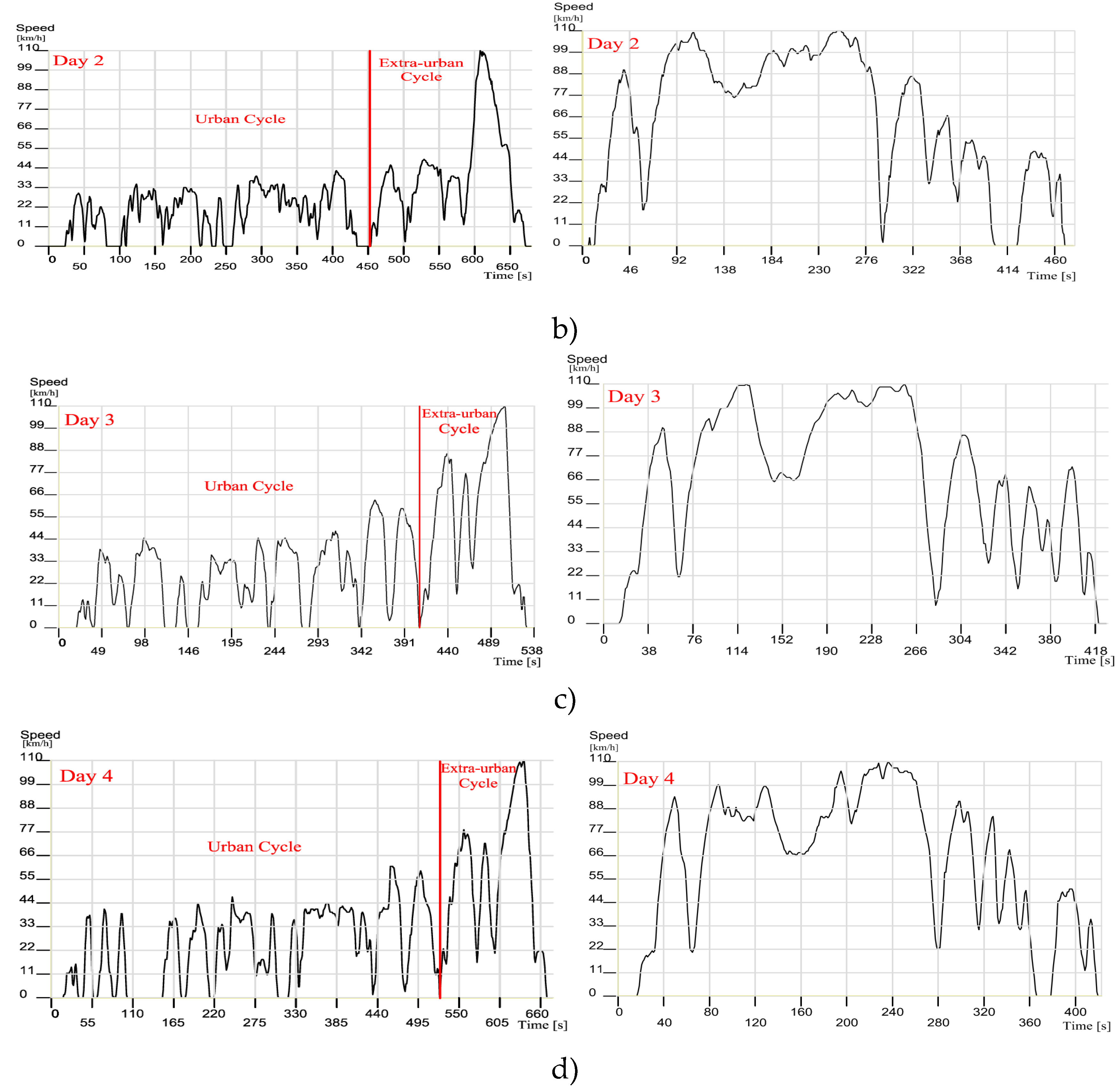
Figure 8.
Variation diagram of NOx, CO and CO2 emissions depending on the thermal regime. a) Vehicle 1, b) Vehicle 2, c) Vehicle 3, d) Vehicle 4.
Figure 8.
Variation diagram of NOx, CO and CO2 emissions depending on the thermal regime. a) Vehicle 1, b) Vehicle 2, c) Vehicle 3, d) Vehicle 4.
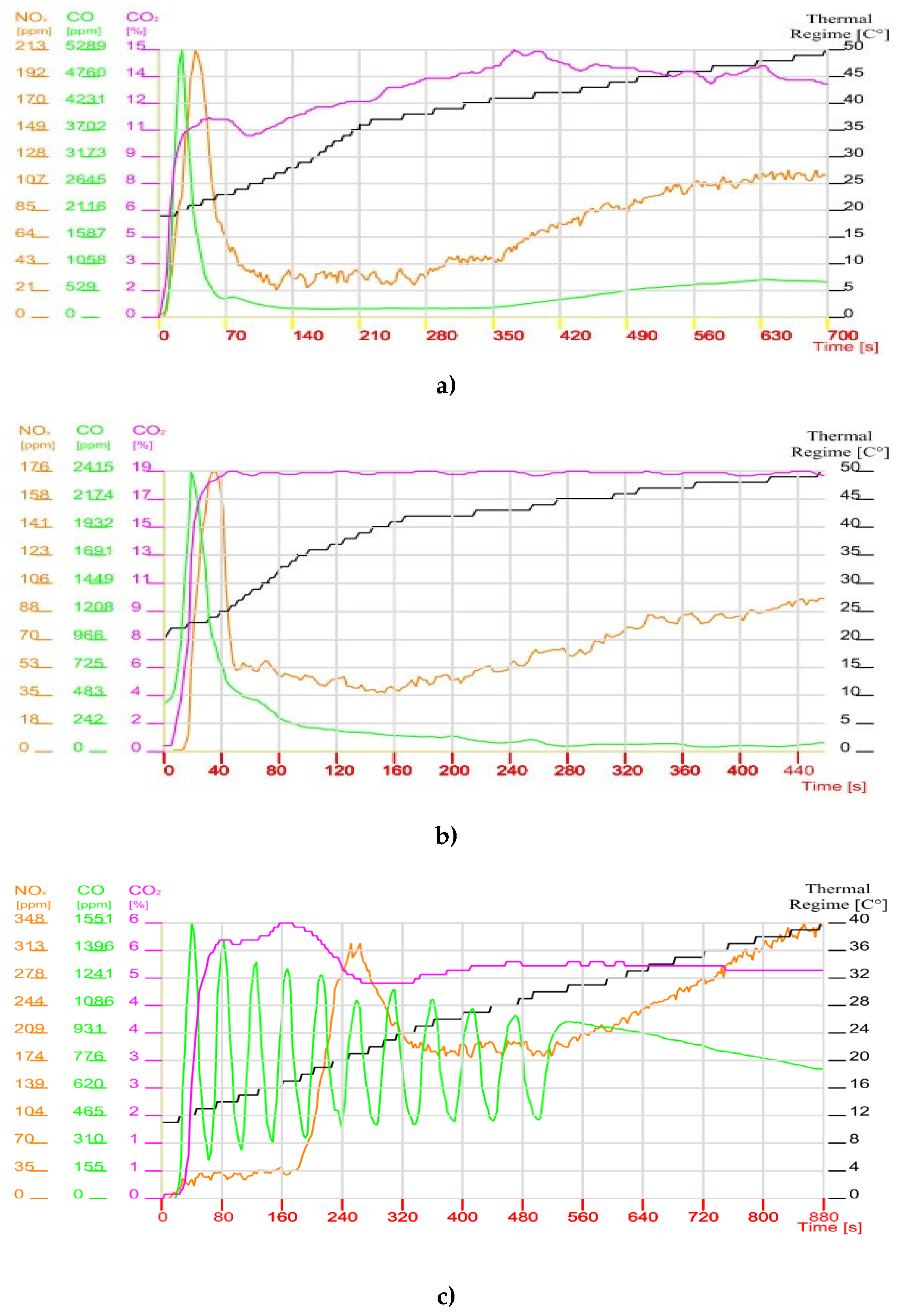
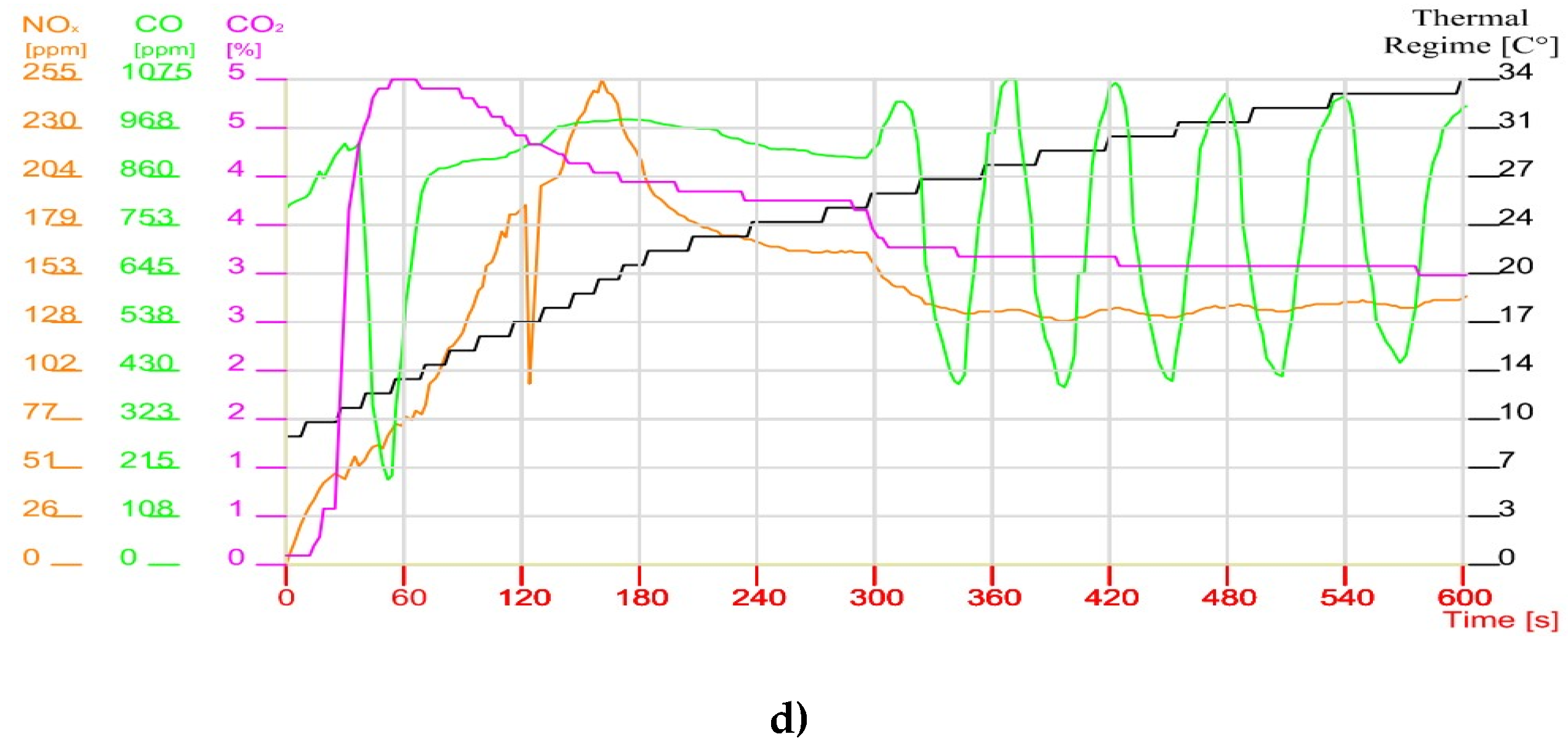
Figure 9.
Emissions variation diagram during the real mixed driving cycle (M-BV Cycle). a) Vehicle 1; b) Vehicle 2.
Figure 9.
Emissions variation diagram during the real mixed driving cycle (M-BV Cycle). a) Vehicle 1; b) Vehicle 2.
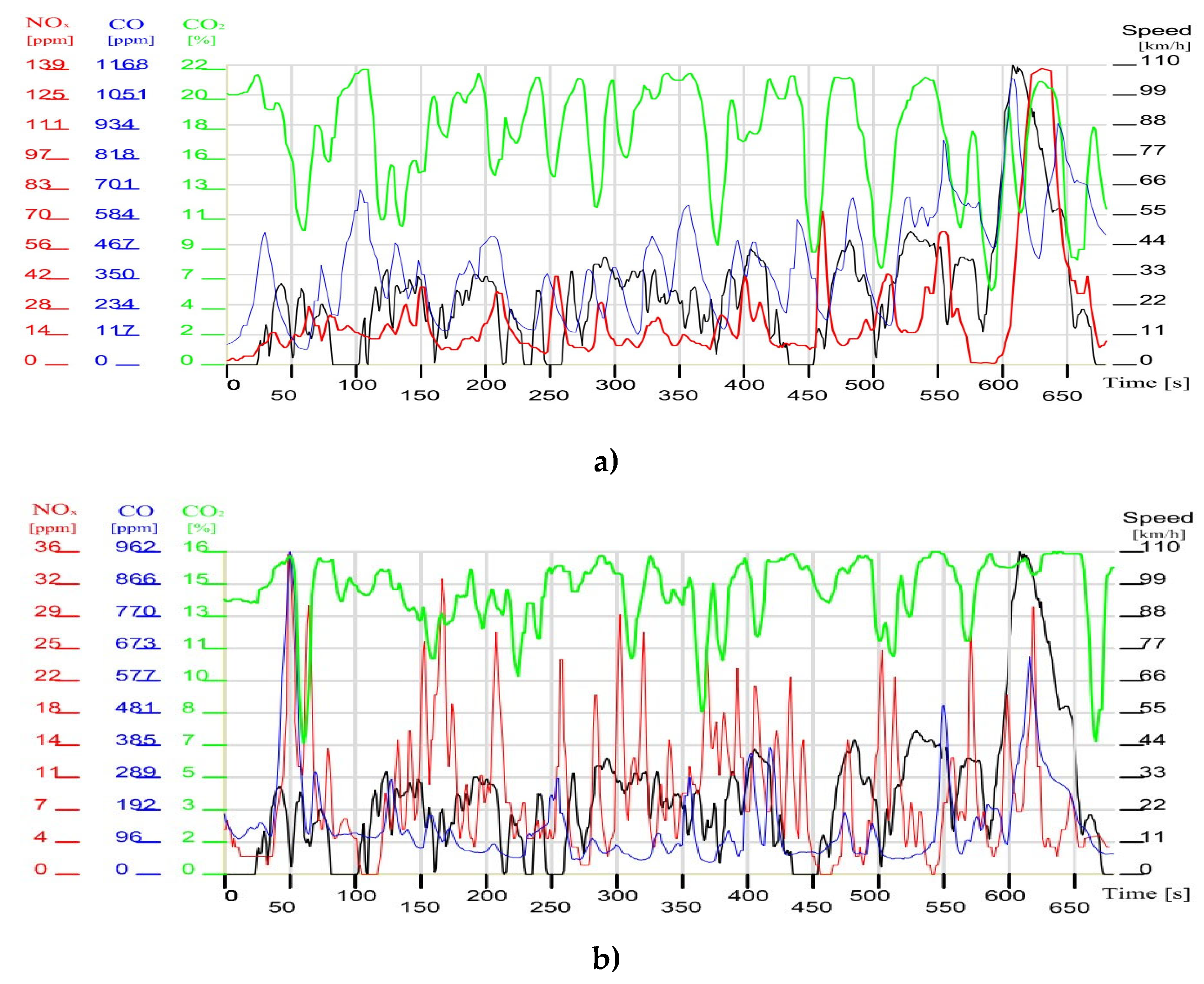
Figure 13.
Fuel consumption variation diagram - mixed driving cycle (”M-BV Cycle”): a) Vehicle 1 and vehicle 2; b) Vehicle 3 and vehicle 4.
Figure 13.
Fuel consumption variation diagram - mixed driving cycle (”M-BV Cycle”): a) Vehicle 1 and vehicle 2; b) Vehicle 3 and vehicle 4.
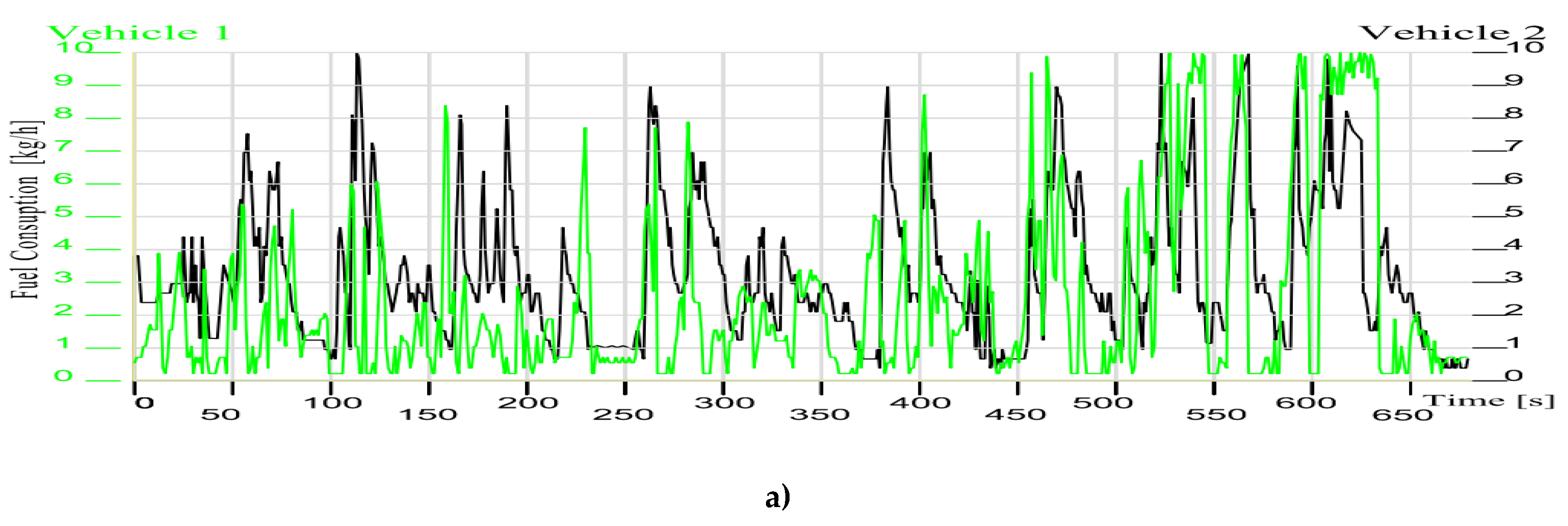
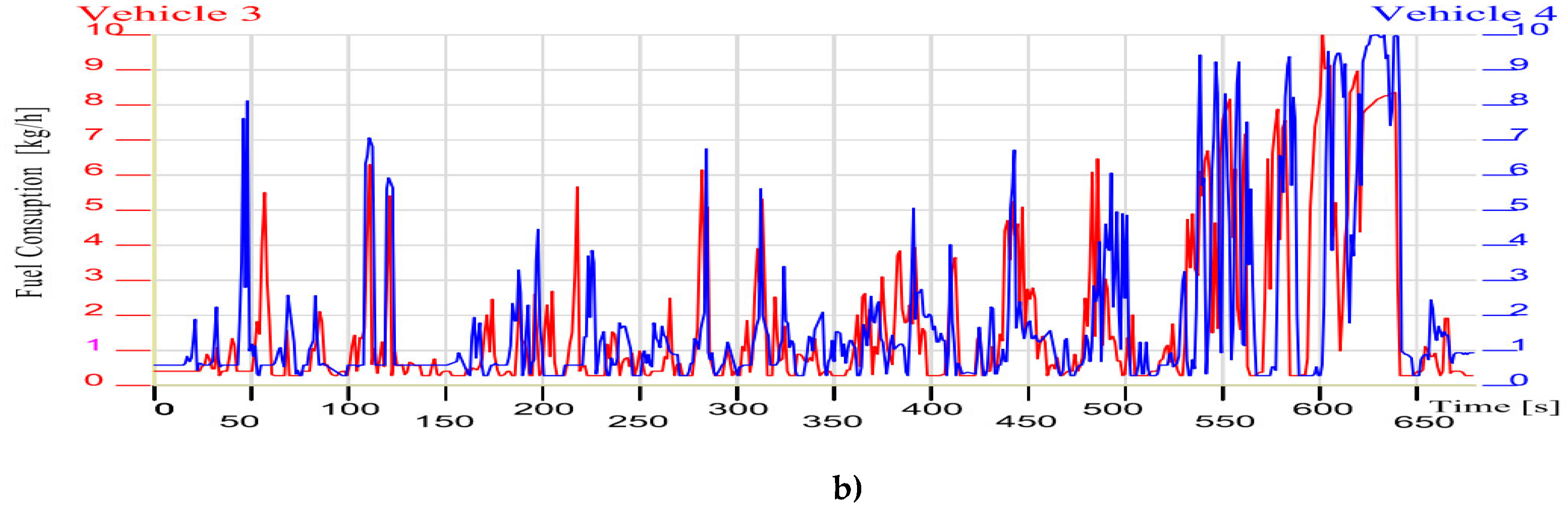
Table 2.
The main technical characteristics of the selected cars for tests.
| Car | Vehicle 1 (SIE) | Vehicle 2 (SIE) | Vehicle 3 (CIE) | Vehicle 1 (CIE) |
|---|---|---|---|---|
| Car Model | SUV | Sedan | Van | Sedan |
| Turbo | Variable geometry | Turbo | ||
| Start & Stop | turbine | Start & Stop | ||
| Catalyst | Three-way catalytic converter |
Three-way catalytic converter |
Oxidation catalyst +SCR |
Oxidation catalyst +SCR |
| Displacement [cm3], (Power [HP]), Gearbox (manual/automatic) | 1.2 PureTech (130 HP), Automatic |
1798 (142 HP), Manual. |
1499 (119HP) Manual |
1461 (75HP) Manual |
| Manufacturing | 2019 | 2017 | 2019 | 2019 |
| Mileage [km] | 30641 | 27321 | 36567 | 33541 |
| Imput parameters-Stand Maha | LPS 3000 MAHA | |||
| Air density [kg/m3] | 1.1 | |||
| The angle of inclination | 0 | |||
| Table of the stand rollers | 200 | |||
| Cf A [KW] | 3.46 | 4.75 | 5.87 | 4.05 |
| Cf B [KW] | 0 | 0 | 0 | 0 |
| Cf C [KW] | 12.38 | 8.75 | 11.2 | 11.92 |
| Mass of vehicle [Kg] | 1050 | 1440 | 1780 | 1229 |
Table 4.
Real driving cycle caracteristic data.
| Mixed Cycles | Extra-Urban Cycles | ||||||||||||
|---|---|---|---|---|---|---|---|---|---|---|---|---|---|
| Cycle characteristics | Day 1 | Day 2 | Day 3 | Day 4 | Day 1 | Day 2 | Day 3 | Day 4 | |||||
| Cycle | M-1 Cycle | M-2 Cycle | M-3 Cycle | M-4 Cycle | E-1 Cycle | E-2 Cycle | E-3 Cycle | E-4 Cycle | |||||
| Distance [km] | 5.4 | 5.4 | 5.4 | 5.4 | 7.1 | 7.1 | 7.1 | 7.1 | |||||
| Time cycle [s] | 610 | 692 | 528 | 682 | 440 | 481 | 425 | 455 | |||||
| Urban | Extra-urban [s] | 460 | 150 | 440 | 252 | 412 | 116 | 528 | 154 | - | - | - | - |
| Number of stops | 4 | 9 | 9 | 9 | 2 | 4 | 2 | 3 | |||||
| Time stops [s] | 33 | 107 | 75 | 120 | 13 | 44 | 17 | 33 | |||||
| Maximum speed [km/h] | 111 | 109 | 110 | 109 | 110 | 110 | 110 | 110 | |||||
| Average speed with stops [km/h] | 31.87 | 28.10 | 36.83 | 28.51 | 58.10 | 53.14 | 60.17 | 56.22 | |||||
| Average speed without stops [km/h] | 33.68 | 33.23 | 42.93 | 34.59 | 59.86 | 58.53 | 62.66 | 60.58 | |||||
Table 7.
The thermal regime of motor vehicles during real driving cycles.
| Vehicle Test | M-BV Cycle | E-BV Cycle |
|---|---|---|
| Vehicle 1 (Gasoline) | 11 - 47 [0C] | 47 - 86 [0C] |
| Vehicle 2(Gasoline) | 10 - 44 [0C] | 44 - 81 [0C] |
| Vehicle 3 (Diesel) | 12 - 37 [0C] | 37 - 69 [0C] |
| Vehicle 4 (Diesel) | 10 - 35 [0C] | 35 - 71 [0C] |
Table 8.
Fuel consumption during real driving cycles and manufacture’ s data.
| Vehicle Test | Vehicle 1 | Vehicle 2 | Vehicle 3 | Vehicle 4 | ||
|---|---|---|---|---|---|---|
| Test fuel consumption | M-BV Cycle | [l/100km] | 16.02 | 19.16 | 13.28 | 13.98 |
| E-BV Cycle | [l/100km] | 14.37 | 11.44 | 16.15 | 15.66 | |
| Manufacturer’s fuel consumption data | Urban travel | [l/100km] | 5.30 | 8.80 | 4.30 | 4.10 |
| Extra urban travel | [l/100km] | 4.00 | 5.60 | 3.30 | 3.80 | |
| Mixed travel | [l/100km] | 4.50 | 6.70 | 3.40 | 3.70 | |
Disclaimer/Publisher’s Note: The statements, opinions and data contained in all publications are solely those of the individual author(s) and contributor(s) and not of MDPI and/or the editor(s). MDPI and/or the editor(s) disclaim responsibility for any injury to people or property resulting from any ideas, methods, instructions or products referred to in the content. |
© 2024 by the authors. Licensee MDPI, Basel, Switzerland. This article is an open access article distributed under the terms and conditions of the Creative Commons Attribution (CC BY) license (https://creativecommons.org/licenses/by/4.0/).
Copyright: This open access article is published under a Creative Commons CC BY 4.0 license, which permit the free download, distribution, and reuse, provided that the author and preprint are cited in any reuse.


