
Submitted:
11 November 2024
Posted:
12 November 2024
You are already at the latest version
Abstract
In the context of discrete-event systems (DESs), critical states usually refer to a system configuration of interest, describing certain important system properties, e.g., fault diagnosability, state/language opacity, and state/event concealment. Technically, a DES is critically observable if an intruder can always unambiguously infer, by observing the system output, whether the plant is currently in a predefined set of critical states or the current state set is disjoint with the critical states. In this paper, given a partially observable DES modeled with a finite-state automaton that is not critically observable, we focus on how to make it critically observable, which is achieved by proposing a novel enforcement mechanism based on differential privacy (DP). Specifically, we consider two observations, where one cannot determine whether a system is currently in the predefined critical states (i.e., the observation violating the critical observability), while the other is randomly generated by the system. When these two observations are processed separately by the differential privacy mechanism (DPM), the system generates an output, exposed to the intruder, that is randomly modified such that its probability approximates the two observations. In other words, the intruder cannot determine the original input of a system by observing its output. In this way, even if the utilized DPM is published to the intruder, he/she is unable to identify whether critical observability is violated.
Keywords:
Discrete event system
; Critical observability
; Differential privacy
MSC: 93C65
1. Introduction
Over the past decade, state estimation in discrete-event systems (DESs) (without a full sensor deployment) has received unprecedented interest thanks to the extensive deployment of cyber-physical systems that are mathematically characterized by discrete-event systems. Within this problem, several core challenges, such as opacity analysis [1,2,3], diagnosability assessment [4,5], detectability verification [6,7], and controller design optimization [8], are deeply dependent on the ability to accurately estimate the system states by its partially observed nature. Particularly, critical observability, as an important concern in the direction of state estimation, is the focus of our exploration in this research. The concept of critical observability, formulated in [9], is widely applied to networked systems, medical & health systems, semiconductor manufacturing, etc. A system is considered to be critically observable if, through the observation of a system output, it is possible to infer without ambiguity whether or not the current system states fully fall into a predefined set of critical states that can characterize several system properties of interest. Petri nets and automata are the main tools for the modeling and control of DESs with potential mutual transformation [10].
There are two commonly employed techniques for checking the critical observability of a DES that is modeled with finite state automata: regular language [11] and observer-based approaches [12,13,14]. In [11], the authors utilize the operations of regular languages to develop a computational procedure to address the observability verification problem, executable in polynomial time. In [12], k-step critical observability is defined and an observer called a k-extended detector is presented to verify k-step critical observability. The critical observability of large-scale finite-state automaton networks is considered in [13] and decentralized critical observers are designed. Lai et al. propose a novel method for constructing observers for polynomially-ambiguous max-plus automata to check their critical observability, which extends earlier work on unambiguous max-plus automata [14].
When a system is verified to be non-critically observable, a significant problem is how to make it critically observable. This research reports a mechanism that, borrowing from DP [15], aims to consolidate/enforce the critical observability for a non-critically observable system. Further, the mechanism ensures that the critical states of the system cannot be detected by an intruder, i.e., achieving critical state protection/concealment.
Differential privacy (DP) is a data processing technique within the field of cryptography, first proposed by Dwork [15]. Building on a solid mathematical foundation, DP guarantees that the statistical characteristics exhibited by the overall dataset will almost remain unchanged when a single entity (a user, a record, or any form of individual data point) is added to or removed from the dataset. In essence, the inclusion/exclusion of a single-record barely alters the computational outcomes of the dataset. Consequently, DP can withstand a wide range of privacy attacks, making it extremely difficult for attackers to accurately infer individual data by observing the calculation results.
The privacy protection mechanism due to DP is primarily achieved by introducing noise to obfuscate the original data during data processing, thereby concealing personal characteristics and sensitive information. The Laplace mechanism [16], which is particularly suited for protecting numerical data, and the exponential mechanism [17], designed for handling non-numerical data, are two of the most common and effective methods for injecting noise in order to implement DP.
As shown in the literature, DP has been widely applied in various fields, including big data analytics, federated learning, recommendation systems, and trajectory data publishing. In [18], DP is combined with the Haar Wavelet technique to protect the privacy of big data in body sensor networks. The authors developed a tree-based structure to analyze the data, reducing errors and enabling long-range queries. In [19], the authors concentrated on three aspects of DP protection for adolescents’ ultrasound examination health datasets: DP protection for basic statistical output perturbations, publication of DP marginal histograms and synthesized data, and machine learning DP learning algorithms. The problem of location and traffic information leakage in vehicular network environments is addressed in [20] by integrating local DP and federated learning. Specifically, the authors introduce four local DPMs, including the three-outputs and optimal piecewise mechanism, to perturb gradients from vehicles, ensuring privacy while maintaining model accuracy and minimizing communication overhead. In [21], Ren et al. employ the data from various social network platforms to generate personalized recommendations, where, to ensure the privacy of the users, DP is applied to the user attributes and the connections present in the social network graph. Presented in [22] and [23] is a privacy protection mechanism for symbolic systems whose traces (symbol sequences) can be protected. Based on this framework, the authors further develop an innovative exponential mechanism. In addition, DP finds its extensive applications in other domains such as logistics [24] and time series trajectories [25]. We believe that more research will be exposed as this kind of privacy protection paradigm prevails corresponding to the increasingly demanding requirements of system security.
Although DP is effective in protecting sensitive information within various information-intensive systems, its potential applications in DESs have yet to be fully explored. This paper primarily focuses on the problem how to utilize DP to enforce critical observability in DESs modeled with finite-state automata. Furthermore, we explore how DP is employed to guarantee that the critical states are not discovered by an intruder. The research follows the schematic illustrated in Figure 1. Specifically, given a system modeled with a nondeterministic finite-state automaton, a set of observable events , a set of critical states , and a set of non-critical states , we assume that the system is not critically observable with respect to (w.r.t.) the predefined set of observable events and critical states . Using the standard determinization procedure presented in [26], we construct a critical state estimator w.r.t. observable events. The system’s behavior can be described as a scenario that the event sequence s generated by is transmitted to the critical state estimator , which then produces an observation .
By estimating the state set that is consistent with an observation , denoted by , we draw a crucial conclusion. If this set is a subset of the non-critical states, i.e., , the observation is regarded as a safe observation. If the set is a subset of the critical states, i.e., , the observation is considered an unsafe observation. In both cases, the critical states can be revealed/detected by an intruder. Otherwise, the set is neither a subset of the critical states nor a subset of the non-critical states, i.e, . In this situation, the observation is also deemed unsafe since the critical observability of the system is violated. In other words, when is acquired by an intruder, he/she can determine that the system is not critically observable. To prevent unsafe observations from being captured, a DP module is introduced as a protection shield. The function of this module is that, when an unsafe observation is received, the module outputs a protected observation with a probability similar to that of another random observation, thereby obscuring the intruder such that it is difficult to trace back to the original unsafe observation. If the observation is safe, the system directly outputs the undecorated .
We further analyze how DP works. For an unsafe observation , it is first mapped into a state sequence , which is a state string interleaved with in , where is the observer of the plant . Then, is sent to the DP module. We assume that the operational logic (running principals) of the DP module is public to an intruder, i.e., the intruder knows the probability distribution of the module generating all possible outputs w.r.t. an input observation . However, when the two state sequences respectively corresponding to an unsafe observation and a random observation are input to the module, the protected output observation is highly similar in probability. This design guarantees that even if an intruder captures , it is difficult to distinguish whether it originates from or , thereby effectively protecting unsafe observations that violate critical observability (i.e., ) or reveal critical states (i.e., ). Under the aforementioned lines, the main contributions of this work are summarized as follows.
(1) A novel framework based on DP for the enforcement of critical observability for DESs is proposed. Given a non-critically observable system, we define an unsafe observation by computing the set of states consistent with it, i.e., an observational system output. In this paper, the designed method aims to confuse the unsafe observations with the randomly generated observations from a probabilistic viewpoint, such that a non-critically observable system satisfies critical observability. Moreover, this method guarantees that the critical states of the system cannot be detected by an intruder.
(2) To expand the application field of DP theory, we propose a new concept, called “state sequence DP” and apply it to finite state automata.
(3) Thanks to the concept of state sequence DP, we design an optimal DPM that ensures the optimal protection of unsafe observations.
The preliminaries of DESs and DP are presented in Section 2. The definition of critical observability is recalled in Section 3. In Section 4, a novel DPM specialized for the enforcement of critical observability of a system is designed. We discuss a realistic case of enforcing critical observability in Section 5 to show the practical applicability of the proposed approach. Finally, concluding remarks are given in Section 6.
2. Preliminaries
The basics of notations and notions necessary for the development of this research are presented, including languages and finite-state machines (deterministic finite automata–DFA and non-deterministic finite automata–NFA), as they are appropriate for the modeling of a DES. A reader is referred to [26]. Note that an NFA is equivalent to a DFA from the lens of languages that they can generate, i.e, they have the same modeling power.
2.1. Languages and Automata
Let E be a finite set of event labels a DES and be a set of the finite strings defined over E (the Kleene closure of set E), consisting of the empty string . Given a string , its length is the number of symbols contained in it, denoted by . In particular, we have . Given two strings and , the string is said to be the concatenation of and .
A DFA is a quadruple , where is the finite set of states, E is, as previously stated, the collection of event labels, is the partially defined deterministic transition function, and is the initial state. In order to facilitate the development of this research, one readily extends the transition function, as again denoted by in the case of no confusion, recursively defined from to , where for and (specifically, we have for all ). Let with be a non-negative integer. We use to denote the set of event sequences with length k, i.e., . Analogously, we write to represent the set of all state sequences with length k. The language generated by is defined as . The set of events that are enabled (feasible) at a given state is defined by . The number of enabled events at state x is thus .
Given a DFA , a sequence (interleaving of states and events) starting from state and ending at a state in , i.e., is said to be a production of with (). We write to represent the set of all productions in the DFA . Given a production of , the state sequence associated with is called a production state sequence, denoted by . Analogously, the event sequence associated with is said to be a production event sequence, is denoted by . Let with be a non-empty state sequence. We write to represent the set of event sequences consistent with . Given a non-empty event sequence with , its consistent state sequence set is defined as . Note that is the set of all finite strings of elements in .
Example 1.
Consider a DFA shown in Figure 2, where and We have , , , , and . Given a production , the production state sequence and the production event sequence associated with ξ are and , respectively. Let us consider an event sequence in . The set of state sequences consistent with is . □
An NFA is a quadruple , where is the finite set of states, E is the same as before explained, is the (partial) transition function, and is the set of initial states. The transition function is similarly extended to by defining for all and , where and . The language generated by from state is formally defined as . Given a set of states , we define . The language of is .
Given an automaton, E is partitioned into two disjoint sets: , where () is the set of observable (unobservable) events. The natural projection is defined by
where and . Function P can be extended to , i.e., given , .
Given an NFA and a state set , the set of states unobservably reached from X is defined as . We use the notation to represent the set of states reached by the occurrence of an observable event from the states in X, i.e., . The observer of , denoted as , can be computed following a standard procedure outlined in [26]. More specifically, is the state set, is the set of observable events, is the (partial) transition function (for all and for all , ), and is the initial state.
Due to the nature of partial observation of a considered plant, we can only observe the observable event labels, while unobservable events can be directly observed. However, different event sequences may have the same observational results. Given an NFA , a string is said to be an observation. The state estimation w.r.t. can be expressed as . By definition, it comes . Note that an observer is a DFA where all events are observable.
2.2. Differential Privacy
Differential privacy is an effective vehicle for privacy protection by providing a mechanism (or a function) to protect sensitive personal information from being disclosed during statistical analysis or data dissemination. Broadly speaking, whenever we use a dataset as the input to this mechanism, the addition or removal of any single record from the dataset will not affect the data query results. This means that even if the dataset is slightly modified, it is difficult or impossible for external intruders to obtain any specific privacy information [15].
Definition 1
(Differential privacy [27]). Let be a positive real number and be a randomized mechanism (function) that takes a dataset as input. Let denote the image of . The mechanism is said to provide -differential privacy if for any two datasets and that differ on a single element, and for any , it holds
where the value of at a dataset or is contained in the sample space, i.e., , with a probability decided by the randomness used in the mechanism, and is the probability of representing the possibility that the output of at belongs to O. ♢
In Definition 1, the performance of DP is evaluated by the value of . Specifically, a smaller indicates a more subtle distinction between the probabilities of events and , signifying a lower likelihood for an intruder to distinguish between the two datasets. Conversely, a larger value of implies a diminished level of protection for users’ private information.
Remark 1.
According to Definition 1, two datasets, namely and , are required to differ in only one element. However, in this study, we extend the concept of DP to the field of DESs modeled with a DFA (the formal definition of DP within the DFAs framework, called state sequence DP, will be presented in Section 4). In the definition of DP tailored for DESs, we define as a mechanism specifically designed for a set of state sequences. The input and output of are two state sequences of equal length. The degree of similarity between these sequences is assessed based on their Hamming distance, as defined in Section 4.
3. Critical Observability for Automata
In this section, we recall the formalization of critical observability verification problems. Given an NFA that is partially observable, i.e., , in practice, certain important physical states of the NFA are called critical states, represented by a subset of states . By acquiring a random sequence of observable events, if an intruder can always unambiguously infer whether the system is currently in a predefined set of critical states, is said to be critically observable.
Definition 2
(Critical observability [13]). Given an NFA , , a set of observable events , and a set of critical states , the system is said to be critically observable w.r.t. and , if the following predicate holds
♢
A critically observable system requires that, for any observation , the state set consistent with the observation should be either a subset of critical states or a subset of non-critical states. To verify whether an NFA is critically observable, one can construct a critical state estimator of , i.e., the observer of , which stores all possible state estimations [26]. Then, a system is critically observable w.r.t. and , if for any state , either or holds.
Let , be an NFA that is not critically observable, be a set of observable events, be a set of critical states, and be the critical state estimator of . The set of critical observability violative states is denoted as .
Example 2.
Consider the NFA shown in Figure 3, where is the set of states, is the set of events with and , and is the set of initial states. The critical state estimator of is portrayed in Figure 4. We assume that the set of critical states is . In Figure 4, by considering an observation , the system is not critically observable w.r.t. and , thanks to , i.e, there exist a state such that and .
However, the NAF is critically observable if the critical state is , since intruders can always determine whether the critical state is reached by observing the system’s behavior. That is, in , for all , or holds. □
Consider a system that is not critically observable w.r.t. the set of observable events and the set of critical states . Let be the critical state estimator of . Given a production of with the observation , if the set of states consistent with is a subset of critical observability violative states or a subset of critical states, i.e., or , the production is said to be unsafe. In this case, the corresponding sequences and are defined as an unsafe production state sequence and an unsafe production event sequence (or an unsafe observation), respectively. Otherwise, the set of states consistent with is included in , i.e., , the production is identified as safe. Its corresponding production event sequence and production state sequence are also considered safe. Once an unsafe observation is exposed to an intruder, he/she can determine that the system is not critically observable or the system’s critical states are revealed. In the following, we focus on how to make a non-critically observable system satisfy critical observability. Moreover, we guarantee that the critical states of the system cannot be revealed by an intruder.
4. Critical State Concealment Based on Differential Privacy
In this section, we aim to design a DPM to enforce critical observability for DESs modeled with DFAs, and to ensure that the predefined critical states cannot be detected to intruders. Specifically, we first define the Hamming distance of two state sequences in a DFA to describe the difference between them. Then, to prevent critical states or critical observability violative states from being captured by an intruder, we define a novel DPM for DFAs, called state sequence DP. Finally, an algorithm that provides a probability distribution for the generation of each state in an output state sequence is proposed and the DPM is designed.
4.1. Problem Statement
In , when an unsafe observation is generated, we can design a DPM associated with to effectively conceal the unsafe observation. In particular, given an observation , we derive its corresponding production state sequence . By inputting and a random production state sequence , such that the Hamming distance between and is restricted to a bound , into the designed mechanism, a protected production state sequence is output with approximate probability, where the lengths of , , and are equal (i.e., ). Since both and can lead to the generation of with probabilities that are sufficiently close, it becomes impossible for an intruder to determine whether or is generated by the estimator . In other words, from the observed behavior contained in , the intruder cannot infer its corresponding input behavior, and thereby the unsafe observation is not identifiable. Before discussing the use of DP to protect unsafe observations from being acquired, we first provide some definitions.
Definition 3
(Hamming distance). Given two production state sequences and generated by a critical state estimator with the same length ( = ), the Hamming distance between and is defined as , where represents the j-th entry of production state sequence , , and . ♢
Let be a critical state estimator of , be a positive integer representing the length of a production state sequence, and be a parameter. We define as the set of all pairs of production state sequences with and the Hamming distance between them is less than or equal to l, i.e.,
Considering Definition 1 and the properties of DES models, we now define state sequence DP in a DFA.
Definition 4
(State sequence differential privacy). Given an NFA , let be its critical state estimator and be the set of state sequences with length k in . Let be a real number. A mechanism is said to be of state sequence DP w.r.t. if for all production state sequence pairs and for all , it holds
where represents the probability of with . ♢
According to Definition 4, a mechanism that guarantees DP of state sequences w.r.t. implies that for all pairs of production state sequences with , and for all possible output production state sequences , the probability of being decorated as and that of being decorated as is close enough such that an intruder cannot identify which is the real input to .
To evaluate the performance of the mechanism, we introduce the concept of the security degree of a state sequence. Given an NFA , a set of observable events , a set of critical states , and the critical state estimator of , let be a state sequence in . If the production state sequence is safe, the security degree of is defined as , where with . Otherwise, the sequence is unsafe, whose security degree is defined as . In other words, the state sequence consistent with an observation that violates critical observability or reveals the critical states (i.e., or ) has the lowest security level. Note that for all , is unique. Given a production state sequence in , a larger value means that the set of critical observability violative states or the set of critical states is less likely to be detected by an intruder.
Consider a critical state estimator of a system and a parameter . The maximum security degree of production state sequences contained in is defined as 1.
Example 3.
Consider the NFA and a set of critical states in Example 2. Let be a production of portrayed in Figure 4 with . The security degree of ω is 2, i.e., . Given another production , the production state sequence is unsafe and has the lowest security degree thanks to . Given a non-negative integer representing the length of a state sequence, we have . □
In this paper, we focus on a mechanism that provides the highest degree of protection for an unsafe production state sequence. In simpler terms, the mechanism is capable of confusing unsafe state sequences with safe ones that have the maximum security degree. In particular, the designed mechanism w.r.t. ensures that, for an unsafe production state sequence , there exists a production state sequence with maximum degree such that and for all .
The distance bound l is another parameter that significantly impacts the performance of the mechanism . Given an unsafe state sequence , it is crucial to select a value l that is as small as possible while guaranteeing that the mechanism can maximally confuse with . In other words, the state sequence , which serves as a suitable alternative for , should exhibit the utmost similarity to .
Definition 5.
Let be an NFA that is not critically observable, be a set of critical states, be a set of observable events, be a critical state estimator of , and be a mechanism that provides state sequence DP w.r.t. . Given an unsafe state sequence , the mechanism is optimal w.r.t. if it satisfies the following statements:
- There exists a production state sequence in with such that , holds;
- For all , the inequality holds;
- For all in with , , there does not exist () such that , . ♢
According to Definition 5, given an unsafe , condition 1) ensures that there exists at least one state sequence with the maximum security degree such that belongs to the set . Condition 2) indicates that an optimal mechanism provides (guarantees) the state sequence DP w.r.t. . Condition 3) implies that the parameter l with must be minimal for all state sequences that satisfy . In the following, we will detail the design of an optimal mechanism that satisfies the definition of state sequence DP.
4.2. State Sequence Differential Privacy
Based on Definitions 4 and 5, we first design a probability allocation strategy for the optimal mechanism in a critical state estimator of system . Given an unsafe input production state sequence , the aim is to generate a random state sequence with a certain probability from such that . Specifically, the strategy to be defined enables assigning a probability to each state included in the output production state sequence , where . Then, by multiplying the probabilities of all output states (), we can obtain the probability of generating , i.e., . In terms of the strategy, we explore the conditions for ensuring the DP of state sequences and further design an algorithm to synthesize this optimal mechanism .
Given a critical state estimator , , let be a mechanism that takes a production state sequence as input and as output. Before elaborating on the probability allocation strategy to a state in , we introduce an indicator function denoted as for two states , defined as follows:
where . If included in satisfies , it is considered a correct state. On the other hand, if , the state is referred to as an incorrect state.
Now, we describe a probability allocation strategy that assigns a probability to each state in the state sequence , where . Given an input production state sequence , let be the set that collects all the states in , i.e., . The strategy for associated with is a (partial) function that outputs a probability of generating state in relation to two states and , where . Particularly, for the initial state, we define , and it is assigned a probability value . Then, for all , if is a correct state, it is allocated a correct probability (the value of is examined in detail in Theorem 1). On the other hand, if is not a correct state, let
| Algorithm 1: A probability Allocation Strategy . |
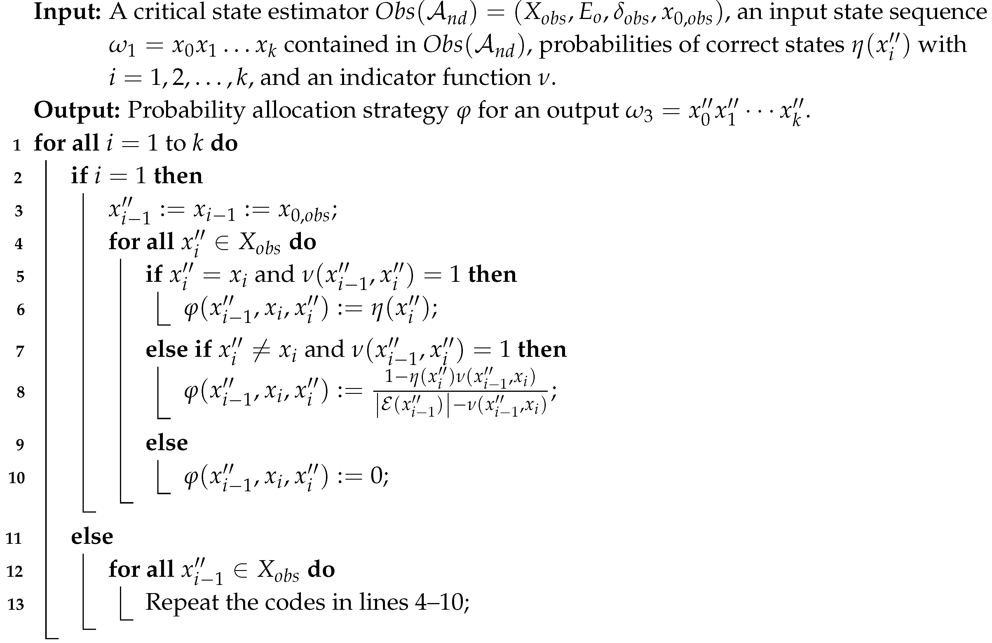 |
Then, we design an algorithm (namely Algorithm 1) to compute the probability allocation strategy for a random output associated with an input state sequence . The algorithm takes as input a critical state estimator, an input state sequence, probabilities of correct states, and an indicator function. It iterates through each state in the input sequence and calculates the probability of generating each possible output state based on the given probabilities of correct states and the indicator function. In Algorithm 1, for all , if , we have . For each possible state , it checks whether and whether the indicator function . If both conditions hold, the correct state is allocated a correct probability . If and the indicator function , the state is assigned an incorrect probability
Otherwise, if , is defined. If , for all , the codes in lines 4–10 are repeated. The computational complexity of Algorithm 1 is .
Example 4.
Consider a state sequence in the critical state estimator in Figure 4 and feed into a mechanism . Let us elaborate on how to calculate the probability allocation strategy φ for a randomly generated output state sequence with (all possible output state sequences with are illustrated in Figure 5).
If , according to the strategy φ, the state is correct and is assigned a correct probability with (the value of is discussed in Theorem 1); if with , by the line 8 of Algorithm 1, we allocate an incorrect probability to state , i.e., .
At the state , since the feasible state is not correct, i.e., and , we have . Analogously, at the state , we have and . □
By utilizing the probability allocation strategy , we are able to synthesize a mechanism that generates a production state sequence assigned with a probability. In other words, for all states contained in , the probability of generating is given by with . Now, we demonstrate the condition of for a mechanism to provide state sequence DP w.r.t. , based on Algorithm 1.
Theorem 1.
Given a critical state estimator of a system that is not critically observable, let be a real number, be a parameter, be the length of a state sequence, be a mechanism whose probability allocation strategy is computed by Algorithm 1, and () be a correct state contained in an output state sequence of . The mechanism guarantees state sequence DP w.r.t. if the probabilities of correct states satisfy the following condition:
Proof. Let and be two production state sequences generated by such that . We consider with (the initial states in , , and are the same, i.e., ). By Definition 4, we need to prove the following inequality:
To begin with, we show . Using Algorithm 1, we have
where and .
Note that when is an incorrect state, the values of depend on , i.e.,
We now claim .
1) First, we prove . One has
2) Let us prove the second inequality .
Then we conclude that
The constraint can be proved similarly, which completes the proof. ▪
By Definition 4 and Theorem 1, Algorithm 2 computes an optimal mechanism for an unsafe input state sequence , which aims to prevent the leakage of critical observability violative states or critical states in a non-critically observable system. [2]We use a number in square brackets after a tuple to represent the entries of the tuple.
[3]A number in square brackets after a set of tuples represents the set contained by the entries of the tuple set. Here, with .
| Algorithm 2: Construction of a mechanism . |
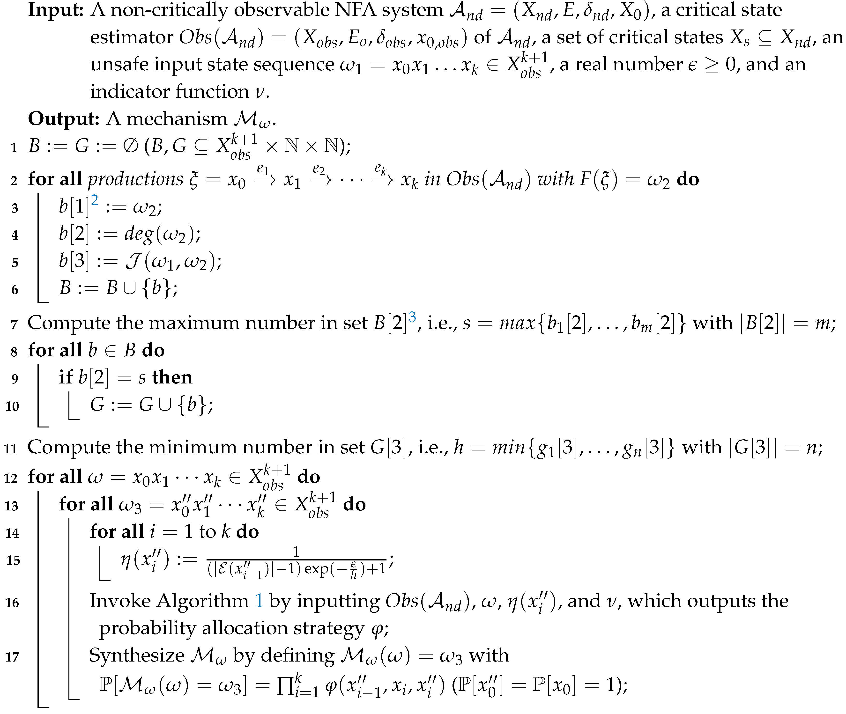 |
Algorithm 2 first initializes two empty sets B and G for storing the triplet elements and . Then, it iterates through all the productions with . In lines 3–6, for each such sequence , the algorithm executes three key computations: assigning , the degree of , and the Hamming distance , to , , and , respectively. In line 7, the maximum value in set is computed and is stored in the variable s. Next, for each triplet b in the set B, check whether is equal to the maximum number s. If the condition is true, then add this element b to the set G. In line 11, the value of the parameter h is obtained by calculating the minimum number in set . For all input state sequences and for all , in line 15, we compute the correct probability for each output state . Finally, in lines 16–17, Algorithm 2 synthesizes the mechanism by invoking the probability allocation strategy of Algorithm 1.
The computational complexity of Algorithm 2 is mainly decided by the synthesis of the mechanism in lines 12–17. In lines 12–13, we enumerate all the input and output sequences, resulting in complexity . Furthermore, in lines 14–16, we compute and utilize Algorithm 1 to calculate . This step has complexity . Taking into account the above statements, the complexity can be expressed as , i.e., .
Theorem 2.
Consider a critical state estimator of a system that is not critically observable. Let be an unsafe production state sequence in . The mechanism computed by Algorithm 2 guarantees DP of state sequences w.r.t. , in which is a parameter calculated by Algorithm 2. Moreover, the mechanism is optimal w.r.t. an unsafe production state sequence .
Proof. First, we prove that the mechanism designed in Algorithm 2 provides DP of state sequences w.r.t. . Specifically, in lines 12–17, for all input state sequences and any possible output state sequence , we have . Besides, we accurately compute the correct state probability based on Equation (2). According to Theorem 1, the mechanism provides DP of state sequences w.r.t. .
Then we show that the mechanism is optimal w.r.t. the unsafe state sequence . In lines 2–6, for all productions , the security degrees of their corresponding state sequences are calculated and these values are stored in the set . Then the algorithm calculates the Hamming distance between and , which reflects the degree of difference between them. In lines 7–10 of the algorithm, elements b are assigned to G such that . In line 11, for all , the minimum value h in the set is obtained, i.e., compute the minimum value h of the Hamming distance between and . To this end, there exists a state sequence with such that and there does not exist such that for all with the maximum degree. According to Definition 5, the mechanism is optimal. ▪
In Algorithm 2, we design an optimal mechanism w.r.t. an unsafe production state sequence . When the mechanism receives as input, a protected state sequence is probabilistically output. In addition, the mechanism guarantees that there exists at least one state sequence with the maximum security degree such that when is fed, it outputs with an approximate probability. Then, when an intruder obtains an observation derived from , he/she is unable to infer whether or is generated in the critical state estimator . Consequently, the disclosure of critical states or critical observability violative states becomes unattainable for the intruder. Furthermore, in order to maximize the obfuscation effect between and , we especially emphasize the optimization of the parameter h in Algorithm 2, i.e., the Hamming distance between and is minimal.
Example 5.
We consider the NFA shown in Figure 3. Based on the results in Example 2 by assuming that the observable event set is and the secret is , the system is not critically observable. Suppose that an unsafe observation is generated, in which the state estimate is neither a subset of the critical states nor a subset of the non-critical states. The unsafe state sequence corresponding to ρ is obtained in the critical state estimator shown in Figure 4. By lines 2–6 of Algorithm 2, we calculate the set B illustrated in Table 1 (the contents of columns 1, 2 and 3 record , and , respectively). Then, we compute the maximum degree of the production state sequences in , i.e., and choose the minimum parameter .
We take the input sequence and a random output for an example. The probabilities of the correct states are
with , where in general . Here, we consider .
By Equation (3), we have
The probability for generating is
Analogously, for another random input state sequence (e.g., with the maximum security degree), we have probabilities for the correct states
When considering as an input of , the probability of generating is
and one has
In other words, if the observation is directly sent, the critical observability violative state can be detected by an intruder due to and . However, by inputting into the designed optimal DPM, a modified state sequence is output. Just by acquiring the sequence , it is difficult for an intruder to backtrack or infer the original sequence , since there exists another random sequence which can also generate with an approximate probability. □
5. Case Study
In this section, we consider a realistic case of enforcing critical observability in air traffic management (ATM) systems. In recent years, with the development of ATM systems, their network architecture has gradually shifted from closed, physically isolated networks to more interconnected and open cyber-physical systems. This evolution has made data exchange and information sharing efficient and convenient, but it has also created more possibilities for potential network attacks. Frequent and diverse types of network attacks pose a serious risk to the safety and stability of aviation. In this context, to strengthen security defenses by enhancing the system’s awareness and response capability to potential threats, we propose an innovative solution: unsafe observations protection based on DP.
An ATM system is illustrated in Figure 6, detailing the communication process between the airport control tower and the pilot during the various stages of flight. On the one hand, the control tower sends a series of instructions to the pilot, such as pre-flight/stop-flight instructions, engine start instructions, etc. These instructions guide the pilot’s actions and determine that the aircraft is airworthy and all parts of the system are operating normally. On the other hand, the pilot’s role is to wait for and follow instructions from the control tower, performing the corresponding operations. If there are any faults or abnormal situations during the flight, the pilot must immediately report to the tower. This real-time feedback mechanism allows the control tower to take action quickly to resolve issues that may threaten flight safety. The exchange of information between the control tower and the pilot runs throughout the entire flight process and jointly affects the aircraft’s maneuvers (represented by the downward arrows in Figure 6). A complete aerial flight can be divided into five stages: taxiing, climbing, cruising, descending, and landing. Each stage requires precise coordination between the pilot and the control tower. Based on Figure 6, we model an ATM system as an NFA (shown in Figure 7) by using a single aircraft as a study case and define a series of important physical states as critical states. The meanings of states and events in the NFA are listed in Table 2. We further assume that an intruder launches an attack as soon as he/she captures the critical states or critical observability violative states. To prevent the system from being corrupted, we introduce a DPM, such that the unsafe states are not accurately captured by an intruder. From a practical standpoint, this research establishes the groundwork for subsequent security defense of cyber-physical systems and has significant implications for safeguarding air transportation safety and maintaining airspace order.
In Figure 7, the pilot initially executes boarding and waits for instructions from the airport control tower (state ). When the pilot receives a pre-flight instruction sent by the tower (event a), the state is transferred from to , at which point the pilot executes a pre-flight check. For any error found by the pilot during the check, an fault is reported (event d) to the tower, and the state is reached. In state , the aircraft is waiting for the engine to start. If the engine fails to start (event e) due to safety issues or other conditions, the state remains in ; otherwise, the state transitions to , where the pilot communicates with the tower in the hope of obtaining a taxi clearance. The taxiing process is represented by states , , and , which correspond to different runways. The event h, obtaining taxi clearance, triggers the transition from to one of these taxing states. Once the taxi clearance is not granted (event n), the state transitions from to or .
The event i, sending a climbing request, triggers the transition from one of the taxiing states (, , or ) to state . If the climb request is granted (event j), the aircraft takes off and leaves the ground (state ). In addition, fault reports (event d) can lead to a transition from to , allowing the aircraft to report any troubles encountered during the flight. However, if the climb request is rejected (event l), the state is switched from to , in which case the flight is stopped and the aircraft returns to its origin. In exceptional cases, the aircraft may be started without authorization, resulting in a move from to , as triggered by event l. In , the pilot sends an anomaly report to the tower (event m), where the aircraft refuses to execute the flight mission and or is reached.
Example 6.
Let us consider the NFA portrayed in Figure 7, where is the set of events with and , and is the set of initial states. We assume that the set of critical states is . The critical state estimator of is shown in Figure 8, where the components of all states are listed in Table 3.
Given an observation , we conclude that the critical observability is violated thanks to and . Therefore, ρ is an unsafe observation and is an unsafe production state sequence.
We now show how the unsafe production state sequence is protected by designed optimal mechanisms that guarantees DP. Consider as an input of . By Algorithm 2, for all , the security degrees and Hamming distances are listed in Table 4. Then we compute the maximum degree and for all with , we select the minimum parameter . For all , and for all , it holds that
where in general . Here, we consider .
When observing , the state that violates critical observability is detectable by an intruder. However, by applying the designed optimal mechanism that outputs a randomly modified production state sequence , the unsafe sequence cannot be ensured, since another sequence with can generate with a similar probability. In this way, unsafe observations in the ATM system cannot be accurately captured. Thereby, the intruder is unable to launch an attack to the ATM system . □
6. Conclusions
This work proposes a differential privacy (DP) mechanism for the enforcement of critical observability in DESs modeled with finite state automata. Meanwhile, the mechanism protects the predefined critical states from being captured by an intruder. We first recall the formalization of critical observability verification problems. Then, a mechanism called state sequence DP is introduced to protect critical states or critical observability violative states such that it cannot be detected by an intruder. Furthermore, in order to most effectively protect unsafe production state sequences, we define an optimal mechanism and design an algorithm for synthesizing the optimal mechanism. Finally, the problem of enforcing critical observability is explored in an ATM system, where model construction of the ATM system and protection implementation of unsafe observations using DP are illustrated in detail.
From a practical perspective, this research has potential applications in various cyber-physical systems. In the future, we will consider applying the differential privacy mechanism to the verification and enforcement of other properties such as k-step and infinite-step opacity. Moreover, it is worth exploring the critical observability problem when a system is subject to sensor attacks, i.e., sensor readings can altered by an external attacker.
References
- Lin, F. Opacity of discrete event systems and its applications. Automatica 2011, 47, 496–503. [Google Scholar] [CrossRef]
- Yang, J.; Deng, W.; Qiu, D.; Jiang, C. Opacity of networked discrete event systems. Inf. Sci. 2021, 543, 328–344. [Google Scholar] [CrossRef]
- Deng, W.; Qiu, D.; Yang, J. Opacity measures of fuzzy discrete Event Systems. IEEE Trans. Fuzzy Syst. 2021, 29, 2612–2622. [Google Scholar] [CrossRef]
- Cao, L.; Shu, S.; Lin, F.; Chen, Q.; Liu, C. Weak diagnosability of discrete-event systems. IEEE Trans. Control. Netw. Syst. 2022, 9, 184–196. [Google Scholar] [CrossRef]
- Liu, F.; Qiu, D. Safe diagnosability of stochastic discrete event systems. IEEE Trans. Autom. Control. 2008, 53, 1291–1296. [Google Scholar] [CrossRef]
- Balun, J.; Masopust, T. On verification of D-detectability for discrete event systems. Automatica 2021, 133. [Google Scholar] [CrossRef]
- Zhu, H.; Liu, G.; Yu, Z.; Li, Z. Detectability in discrete event systems using unbounded Petri nets. Mathematics 2023, 11. [Google Scholar] [CrossRef]
- Li, Y.; Wang, M.; Jones, A. An approach for the design of supervisory controller of discrete event systems. 3rd World Congress on Intelligent Control and Automation, 2000, pp. 2341–2346.
- De Santis, E.; Di Benedetto, M.D.; Di Gennaro, S.; D’Innocenzo, A.; Pola, G. Critical observability of a class of hybrid systems and application to air traffic management. In Stochastic Hybrid Systems: Theory and Safety Critical Applications; 2006; pp. 141–170.
- Zhu, G.; Yin, L.; Li, Y.; Li, Z.; Wu, N. Identification of labeled Petri nets from finite automata. Inf. Sci. 2024, 667, 120448. [Google Scholar] [CrossRef]
- Di Benedetto, M.D.; Di Gennaro, S.; D’Innocenzo, A. Discrete state observability of hybrid systems. Int. J. Robust Nonlinear Control 2009, 19, 1564–1580. [Google Scholar] [CrossRef]
- Tong, Y.; Ma, Z. Verification of k-step and definite critical observability in discrete-event systems. IEEE Trans. Autom. Control 2023, 68, 4305–4312. [Google Scholar] [CrossRef]
- Pola, G.; De Santis, E.; Di Benedetto, M.D.; Pezzuti, D. Design of decentralized critical observers for networks of finite state machines: A formal method approach. Automatica 2017, 86, 174–182. [Google Scholar] [CrossRef]
- Lai, A.; Lahaye, S.; Komenda, J. Observer construction for polynomially ambiguous max-plus automata. IEEE Trans. Autom. Control 2022, 67, 1582–1588. [Google Scholar] [CrossRef]
- Dwork, C. Differential privacy. International Colloquium on Automata, Languages, and Programming. Springer, 2006, pp. 1–12.
- Dwork, C.; McSherry, F.; Nissim, K.; Smith, A. Calibrating noise to sensitivity in private data analysis. 3rd Theory of Cryptography Conference. Springer, 2006, pp. 265–284.
- McSherry, F.; Talwar, K. Mechanism design via differential privacy. 48th Annual IEEE Symposium on Foundations of Computer Science. IEEE, 2007, pp. 94–103.
- Lin, C.; Wang, P.; Song, H.; Zhou, Y.; Liu, Q.; Wu, G. A differential privacy protection scheme for sensitive big data in body sensor networks. Ann. Telecommun. 2016, 71, 465–475. [Google Scholar] [CrossRef]
- Li, W.; Wang, S.; Wang, H.; Lu, Y. Child health dataset publishing and mining based on differential privacy preservation. Mathematics 2024, 12. [Google Scholar] [CrossRef]
- Zhao, Y.; Zhao, J.; Yang, M.; Wang, T.; Wang, N.; Lyu, L.; Niyato, D.; Lam, K.Y. Local differential privacy-based federated learning for internet of things. IEEE Internet Things J. 2021, 8, 8836–8853. [Google Scholar] [CrossRef]
- Ren, J.; Jiang, L.; Peng, H.; Lyu, L.; Liu, Z.; Chen, C.; Wu, J.; Bai, X.; Yu, P.S. Cross-network social user embedding with hybrid differential privacy guarantees. 31st ACM International Conference on Information and Knowledge Management, 2022, pp. 1685–1695.
- Jones, A.; Leahy, K.; Hale, M. Towards differential privacy for symbolic systems. 2019 American Control Conference, 2019, pp. 372–377.
- Chen, B.; Leahy, K.; Jones, A.; Hale, M. Differential privacy for symbolic systems with application to Markov Chains. Automatica 2023, 152. [Google Scholar] [CrossRef]
- Kang, H.; Zhang, S.; Jia, Q. A method for time-series location data publication based on differential privacy. Wuhan University Journal of Natural Sciences 2019. [Google Scholar] [CrossRef]
- Hua, J.; Gao, Y.; Zhong, S. Differentially private publication of general time-serial trajectory data. 2015 IEEE Conference on Computer Communications, 2015.
- Cassandras, C.G.; Lafortune, S. Introduction to Discrete Event Systems; Springer, 2009.
- Dwork, C.; Roth, A. The algorithmic foundations of differential privacy. Foundations and Trends in Theoretical Computer Science 2014, 9, 211–406. [Google Scholar] [CrossRef]
| 1 | The notation (or ) applied to a set represents the maximum (or minimum) element contained in the set. |
Figure 1.
Framework of critical state concealment.
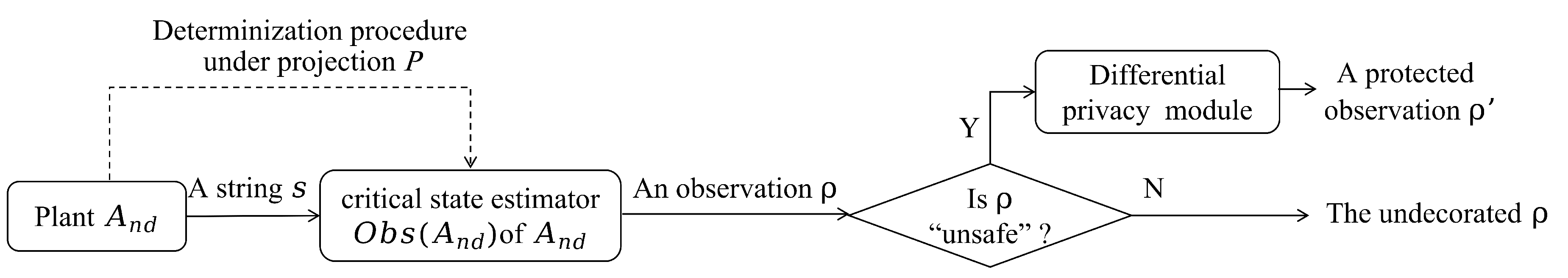
Figure 2.
DFA .
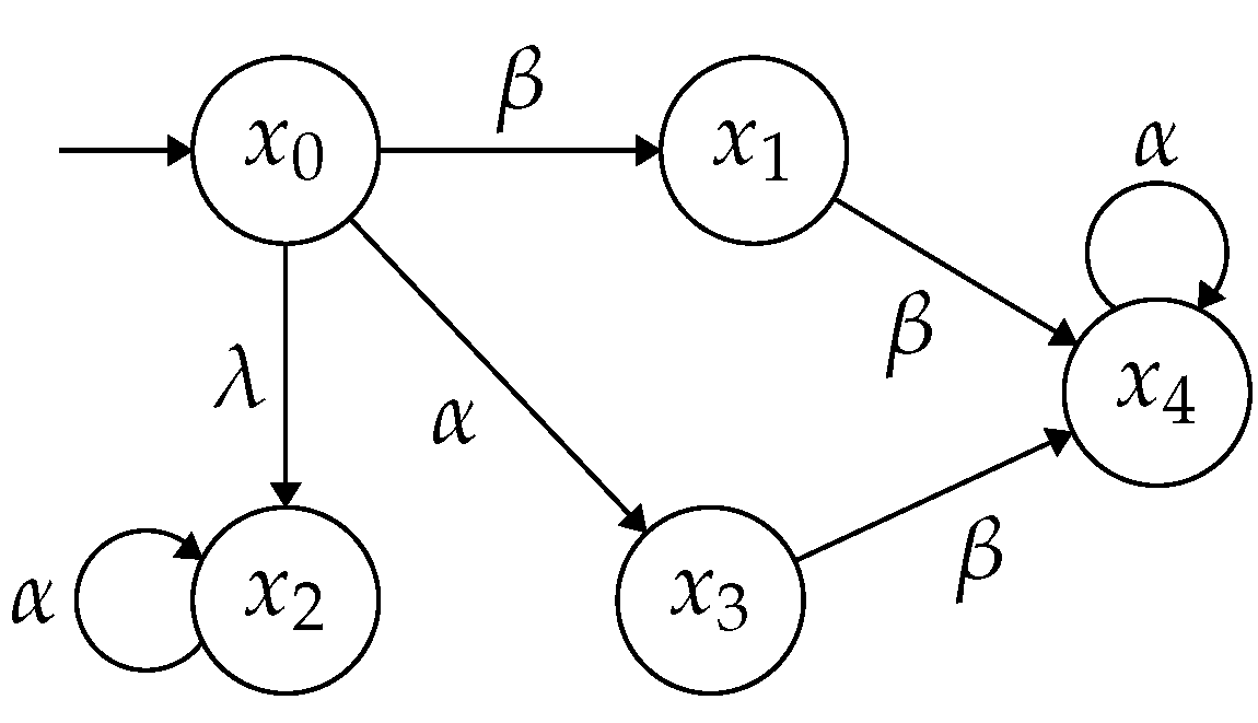
Figure 3.
NFA .
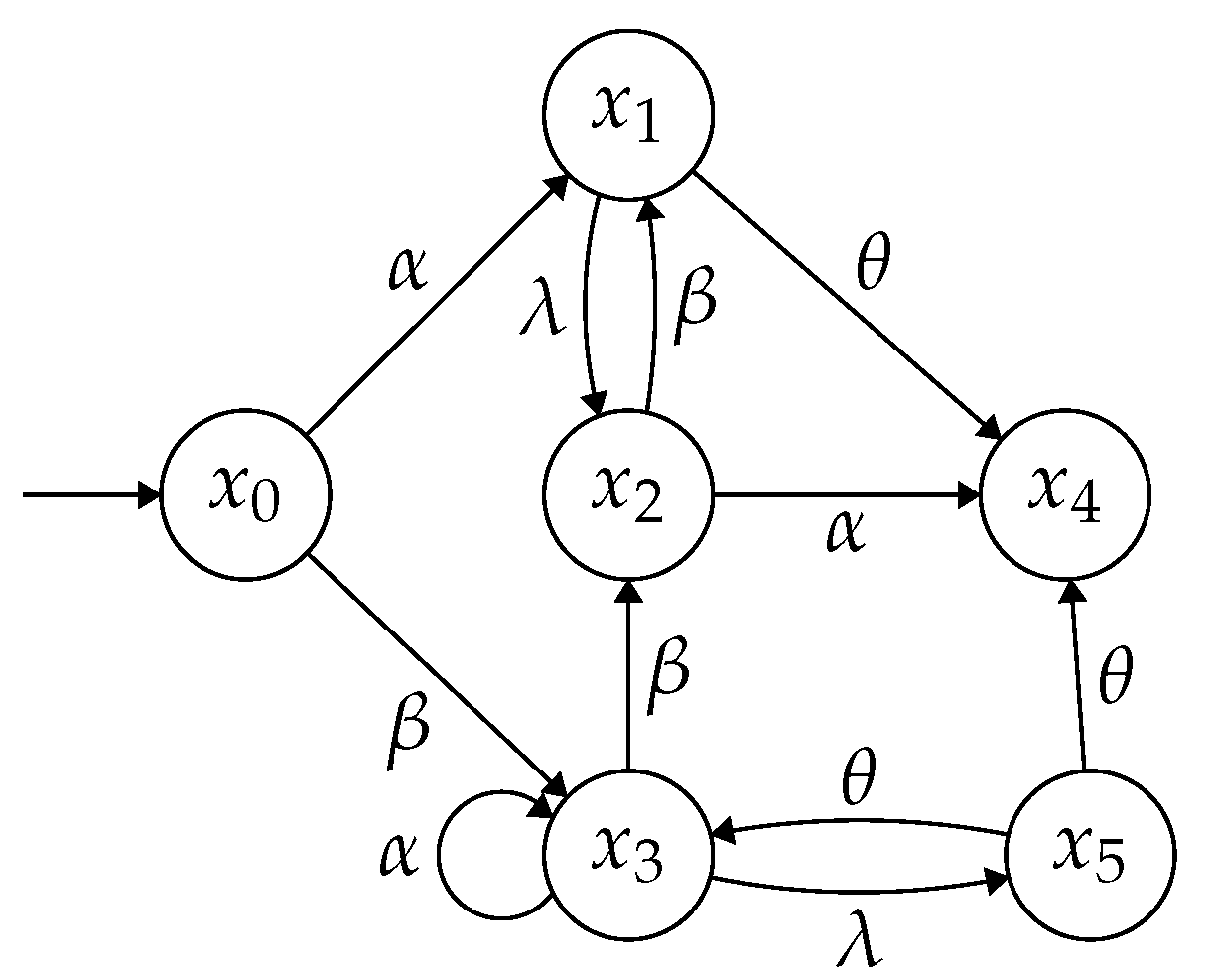
Figure 4.
Critical state estimator of .
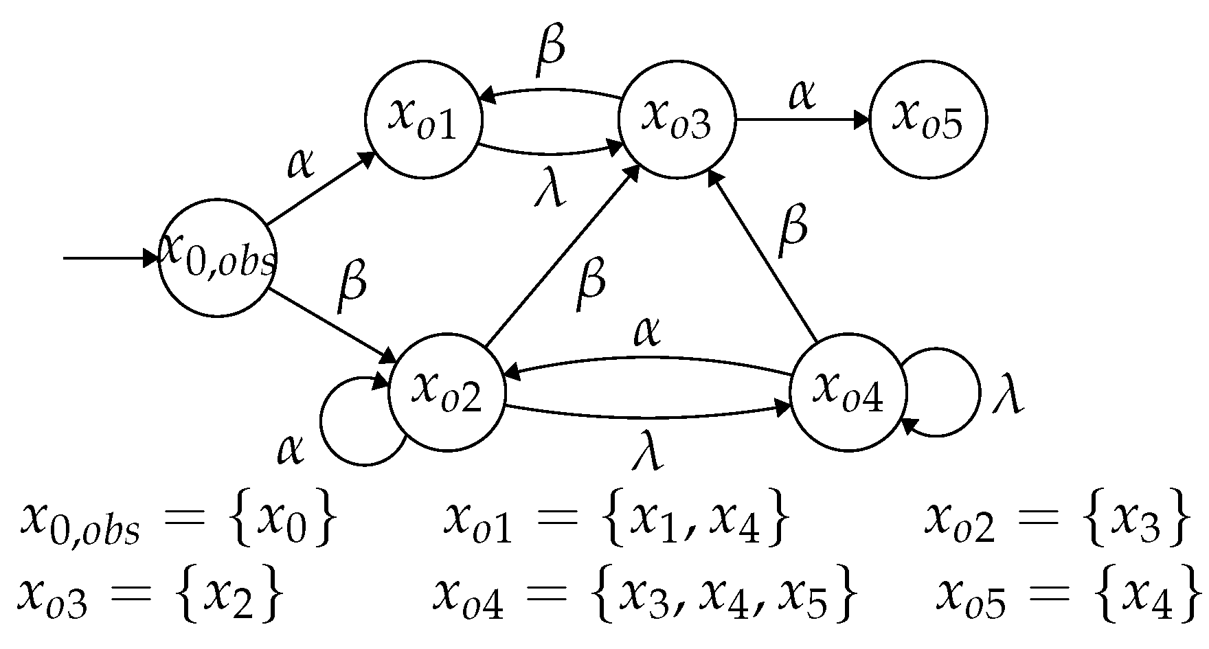
Figure 5.
Probability allocation strategy for all possible output production state sequences .
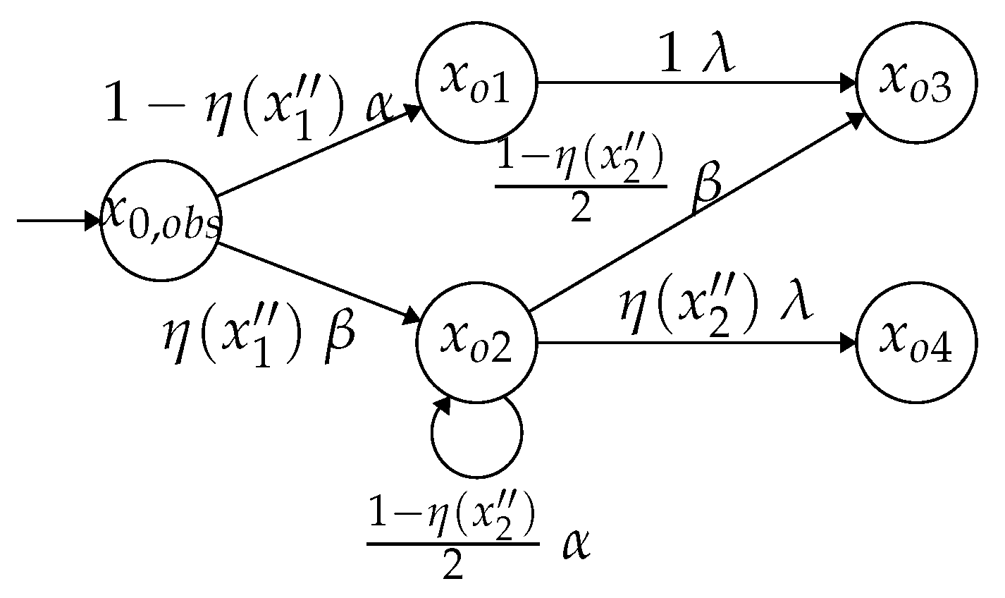
Figure 6.
Air traffic management systems.
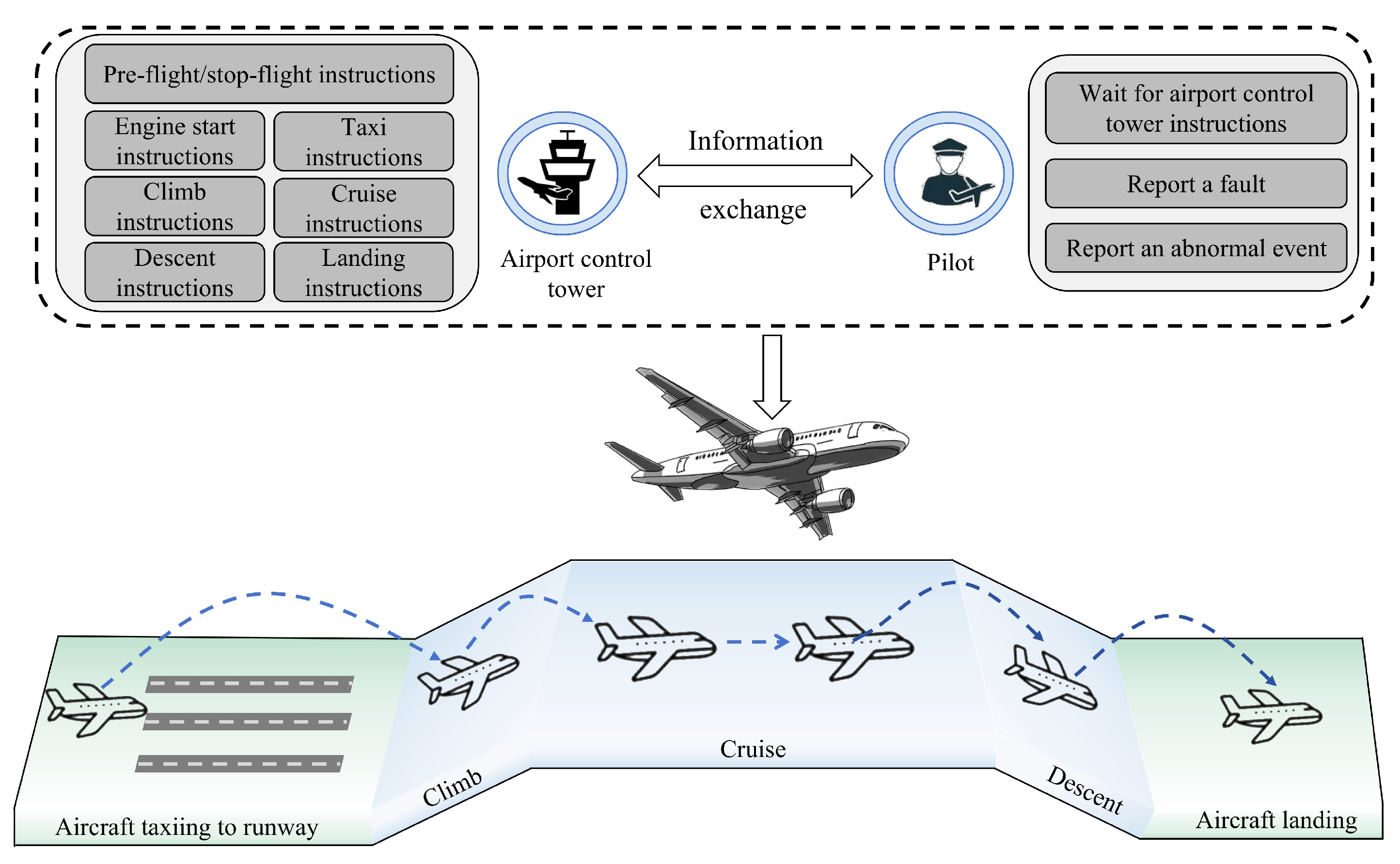
Figure 7.
An NFA model of an air traffic management system.
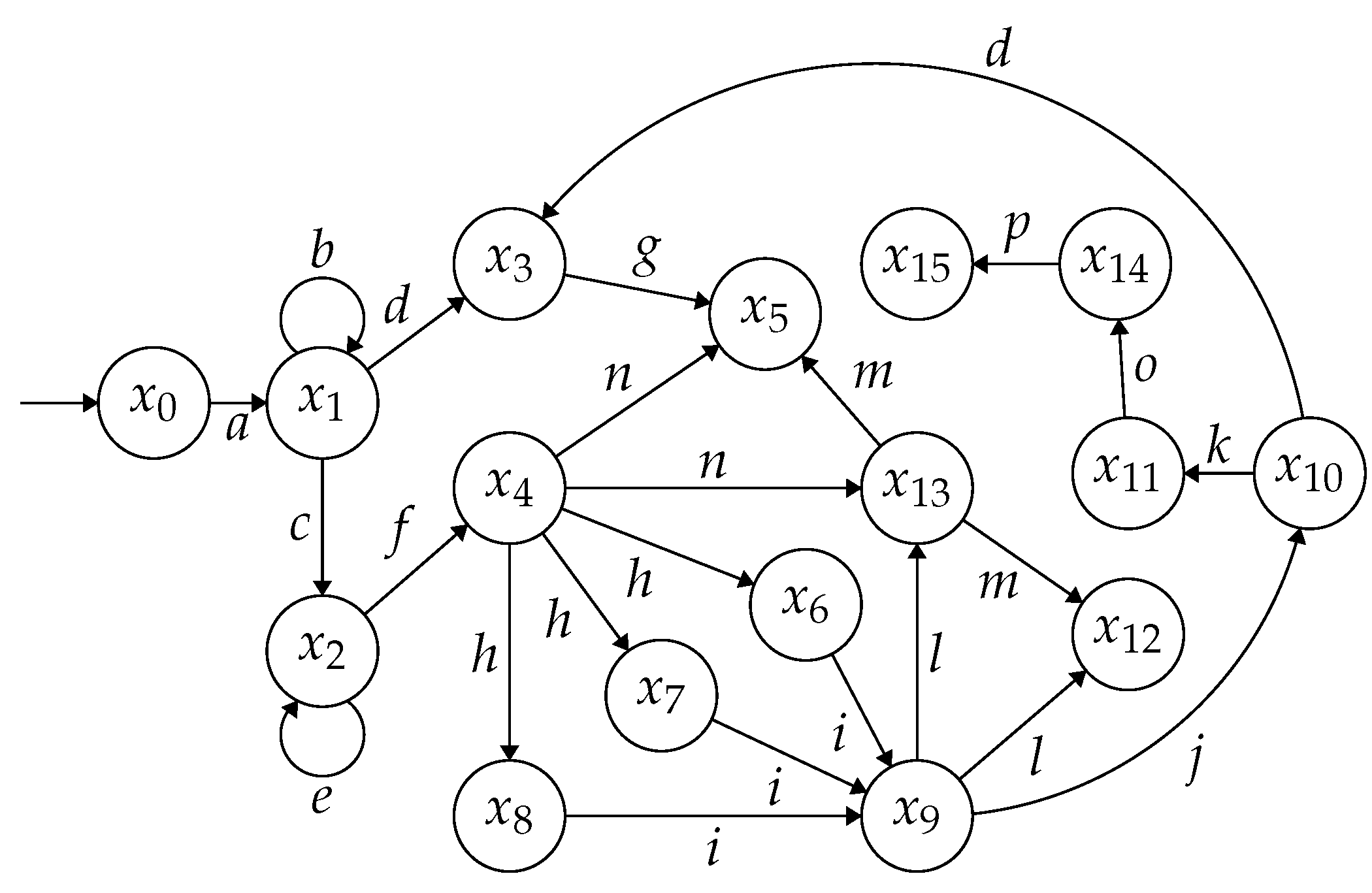
Figure 8.
The critical state estimator of the air traffic management system .
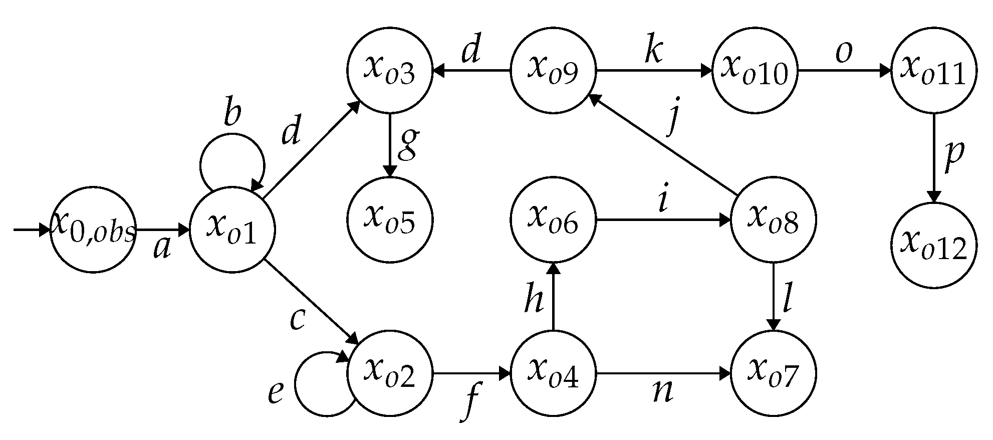

Table 1.
Components of the set B in Example 5.
| States Sequence | Security | Hamming |
| Degree | Distance | |
| 0 | 1 | |
| 1 | 2 | |
| 1 | 1 | |
| 1 | 2 | |
| 0 | 1 | |
| 0 | 2 | |
| 2 | 3 | |
| 1 | 3 |
Table 2.
Meanings of states and events of the NFA portrayed in Figure 7.
Table 2.
Meanings of states and events of the NFA portrayed in Figure 7.
| state | Meanings of states | event | Meanings of events |
| Pilot boards an aircraft and waits for instructions | a | Send a pre-flight instruction | |
| Pilot executes a pre-flight check | b | Incomplete pre-flight check | |
| Waiting for the engine to start | c | Complete pre-flight check | |
| Fault reports are received | d | Send a fault report | |
| Waiting for taxi clearance | e | Reject engine start | |
| Rejected take off | f | Allow engine start | |
| Aircraft taxiing to runway | g | Send stop-flight instructions | |
| Aircraft taxiing to runway | h | Obtain taxi clearance | |
| Aircraft taxiing to runway | i | Send a climb request | |
| Aircraft waiting for authorization at the runway | j | Climb request granted | |
| Aircraft take off | k | Send a cruise instruction | |
| Aircraft cruise | l | Climb request rejected | |
| Stop flight and return to origin | m | Send an anomaly report | |
| Aircraft started without authorization | n | Taxi clearance not granted | |
| Aircraft descent | o | Send a descent instruction | |
| Aircraft landing | p | Send a landing instruction |
Table 3.
Components of the states in the estimator shown in Figure 8.
Table 3.
Components of the states in the estimator shown in Figure 8.
| state | state estimation | state | state estimation |
Table 4.
All production state sequences with length 5 in .
| States Sequence | Security | Hamming |
| Degree | Distance | |
| 1 | 3 | |
| 1 | 3 | |
| 1 | 3 | |
| 0 | 3 | |
| 1 | 3 | |
| 1 | 3 | |
| 1 | 2 | |
| 1 | 2 | |
| 3 | 1 |
Disclaimer/Publisher’s Note: The statements, opinions and data contained in all publications are solely those of the individual author(s) and contributor(s) and not of MDPI and/or the editor(s). MDPI and/or the editor(s) disclaim responsibility for any injury to people or property resulting from any ideas, methods, instructions or products referred to in the content. |
© 2024 by the authors. Licensee MDPI, Basel, Switzerland. This article is an open access article distributed under the terms and conditions of the Creative Commons Attribution (CC BY) license (http://creativecommons.org/licenses/by/4.0/).
Copyright: This open access article is published under a Creative Commons CC BY 4.0 license, which permit the free download, distribution, and reuse, provided that the author and preprint are cited in any reuse.


