
Submitted:
23 October 2024
Posted:
23 October 2024
You are already at the latest version
Abstract
As network systems become larger and more complex, there is an increasing focus on how to verify the security of systems that are at risk of being attacked. Automated penetration testing is one of the effective ways to do this. Uncertainty caused by adversarial relationships and the "fog of war" is an unavoidable problem in penetration testing research. However, related methods have largely focused on the uncertainty of state transitions in the penetration testing process, and have generally ignored the uncertainty caused by partially observable conditions. To address this new uncertainty introduced by partially observable conditions, we model the penetration testing process as a partially observable Markov decision process (POMDP), and propose an intelligent penetration testing decision method compatible with it. We experimentally validate the impact of partially observable conditions on penetration testing. The experimental results show that our method can effectively mitigate the negative impact of partially observable conditions on penetration testing decision. It also exhibits good scalability as the size of the target network increases.
Keywords:
penetration testing
; partially observable problems
; Modeling and intelligent decision
; partially observable markov decision process
; observational locality
; observational uncertainty
1. Introduction
As network systems become larger and more complex, there is an increasing focus on how to verify the security of systems that are at risk of being attacked. Automated penetration testing is one of the effective ways to do this. Traditional Penetration Testing (PT) relies on manual approaches that become impractical as systems grow in size and complexity. Automated penetration testing technologies simulate real attackers with attack strategies and use various algorithmic models to automate the penetration of target networks, significantly reducing testing costs and increasing penetration efficiency [1,2].
Due to the adversarial nature between attackers and defenders, the ability to accurately observe the whole situation is often lacking, resulting in the failure of classical decision algorithms. The study of modelling and decision methods under partially observable conditions in these adversarial environments is of critical importance [3].
Studies on penetration testing decision typically model the penetration testing process by constructing a Markov Decision Process (MDP), which is a traditional mathematical tool for formalizing process dynamics and state transition uncertainty. However, it lacks sufficient consideration for partially observable problems.
To address this issue, we model the penetration testing process as a Partially Observable Markov Decision Process (POMDP). In addition to process dynamics and state transition uncertainty, we extend the modelling of observational locality and observational uncertainty, thereby strengthening the formal expression of partially observable problems. Correspondingly, a compatible intelligent decision method is proposed that combines deep reinforcement learning and recurrent neural networks. By exploiting the characteristics of recurrent neural networks in handling sequential data and the advantages of deep reinforcement learning in exploring and learning unknown systems, the method can effectively mitigate the negative impact of partially observable conditions on penetration testing decision.
The main contributions of this paper are as follows:
- Formalising the penetration testing process as a partially observable markov decision process, allowing the exploration and study of observational locality and observational uncertainty in adversarial scenarios. This approach is more in line with the realities of the ’fog of war’ and the subjective decision process based on observations in the field of intelligent decision.
- To address the new uncertainty challenges posed by partially observable conditions, an intelligent penetration path decision method based on the combination of deep reinforcement learning and recurrent neural networks is proposed. This method enhances the learning capability of sequential attack experience under partially observable conditions.
2. Related Works
Automated penetration testing is a significant application of artificial intelligence technology in the field of cybersecurity [4]. Methods based on reinforcement learning, by designing the success probability of action execution, can simulate real-world uncertainties in attack and defense, making it a crucial research direction in this domain. Schwartz et al. [5] designed a lightweight network attack simulator, NASim, providing a benchmark platform for network attack-defense simulation testing. They validated the application effectiveness of fundamental reinforcement learning algorithms like Deep Q-learning Network(DQN) in penetration path discovery. Zhou Shicheng et al. [6] proposed an improved reinforcement learning algorithm, Noisy-Double-Dueling DQN, to enhance the convergence speed of DQN algorithms in the context of path discovery problems. Hoang Viet Ngueyen et al. [7] introduced an A2C algorithm with a dual-agent architecture, responsible for path discovery and host exploitation, respectively. Zeng Qingwei et al. [8] suggested the use of a hierarchical reinforcement learning algorithm, addressing the problem of separate processing for path discovery and host exploitation.
Methods based on reinforcement learning often formalize the penetration testing process as a Markov Decision Process (MDP). While these methods describe the dynamism of the penetration testing process and the uncertainty of state transitions, they do not effectively model the observational locality and observational uncertainty in the network attack-defense "fog of war". Therefore, related studies pay attention to model partially observable conditions in penetration testing [9]. Sarraute et al. [10] incorporated the information gathering stage of the penetration testing process into the penetration path generation process, achieving the automation of penetration testing for individual hosts for the first time. Shmaryahu et al. [11] modeled penetration testing as a partially observable episodic problem and designed the episodic planning tree algorithm to plan penetration paths. The aforementioned solving methods do not give detailed analysis and general models of partially observable problems, nor do they consider integration with intelligent methods to support automated testing.
Based on the above studies, we further investigate the impact of partially observable conditions on penetration testing. We analyse and model the partially observable problems in penetration testing from two aspects of observational locality and observational uncertainty, and integrate them with MDP. Based on this, we propose an intelligent decision method to enhance the learning ability of sequential attack experience under partially observable conditions.
3. Problem Description and Theoretical Analysis
Figure 1 shows a typical penetration testing scenario, which we use as a case study to illustrate the issue addressed in this paper. The target network consists of 4 subnets, each containing several hosts, including sensitive hosts. The role of the PT decision method is to decide, based on state observation, the attack targets at each step and plan the optimal attack path to maximise the attack reward. In this scenario, the goal is to intelligently achieve the highest privileges on hosts (2,0) and (4,0) with the fewest attack steps, while avoiding host (3,2) to avoid triggering the negative reward associated with the honeypot.
The MDP is typically modelled as a quadruple , where S denotes the set of penetration states observed by the agent, such as network topology, host information, and vulnerability details. A is the set of attack actions available to the PT agent, such as network scanning, host scanning, vulnerability exploitation, privilege escalation, etc. R is the reward function , which corresponds to the reward for different penetration states, for example, the reward for obtaining the highest privileges on host (2,0) is 100, and the reward for attempting to attack host (3,2) is -100. P denotes the state transition function , typically associated with the success rate of the attack actions. The goal of the MDP is to select the optimal policy to optimise the long-term cumulative reward for the current state, as in (1).
where denotes the discount factor, used to balance the importance of current rewards against future rewards.
The MDP formalises the process dynamics and state transition uncertainty of penetration testing, but assumes accurate observability, where the state observed by the PT agent matches the actual state:. However, the existence of adversarial relationships and the "fog of war" makes this assumption impractical. On the one hand, the PT agent cannot directly obtain a global perspective, but gradually explores the topology and host information as it moves laterally through the penetration. On the other hand, the application of moving target defense and deceptive defense methods may also introduce inaccuracies in the observed state.
Therefore, in this paper we make more realistic assumptions: , indicating that the PT agent has observational locality and observational uncertainty, which means the observed state not only partially but also may have some degree of deviation.
In this paper, we model the penetration testing process as a Partially Observable Markov Decision Process (POMDP), taking into account the observational locality and observational uncertainty of the PT agent. The actual penetration process still relies on the foundation of the MDP quadruple, but replaces the set of attack actions A with the intelligent agent model , denoted as . And the intelligent agent model is further defined as , where O is the observation function, , which describes the observational locality and the observational uncertainty. A denotes the set of available attack actions for the PT agent. denotes the decision strategy of the PT agent based on the observed state:. The goal is to select the optimal strategy based on the partially observed state of the PT agent, rather than the actual state , in order to optimise the long-term cumulative reward for the current state, as in (2).
In our model, the actual state still evolves based on objective attack actions and an objective state transition function. However, the observation and decision components of the PT agent are treated independently. They are replaced by observed states , which may differ from the actual states, and decisions are made based on observed states. This aligns more closely with actual "fog of war" scenarios and better simulates the subjective decision process based on observations, which is the main innovation of this paper.
4. Methodology
4.1. POMDP Modelling
4.1.1. State Modelling
Typically, related studies have modelled the state space by different stages of the penetration process. However, as the penetration stage is a state concept from a global perspective, which contradicts the partially observable conditions. Therefore, we propose a new state modelling to describe the penetration state based on the feedback obtained from each action of the PT agent. In the penetration process, the primary feedback consists of the target host information and its changes. Thus, we model the penetration state based on the information of each host and derive the observation state for the PT agent. The information for each host includes topological location, compromise information, operating system details, service details and process details. Different types of information are encoded and identified using one-hot vectors. The dimensions of the encoding are determined based on the estimated size and complexity of the specific scenario. In the scenario shown in Figure 1, where the total number of subnets is 4, the corresponding field dimensions can be set to any dimension greater than 4. Larger dimensions provide more capacity for our method. However, accurate estimation contributes to modelling accuracy and efficiency.
Using the scenario in Figure 1 as an example, the modelling of host information is as follows:
- Topological location information: Topological location information includes subnet identifiers and host identifiers. For the scenario in Figure 1, the capacity of the subnet identifier field can be set to 4 and the capacity of the host identifier field can be set to 5. Thus, the dimension of the topological location field is 9, with the first 4 dimensions identifying the subnet in which the target host is located, and the remaining 5 dimensions identifying the location of the host within the subnet. For example, the topological location encoding for the honeypot host (3,2) is (0010 00100).
- Compromised state information: Compromised state information is encoded by a 6-dimensional vector, including whether compromised, accessible, discovered, compromise reward, discovery reward and compromised privileges (user or root).
- Operating system, service, and process information: These three categories of information are closely related to vulnerabilities and attack methods. In the scenario shown in Figure 1, the target host is configured with 2 types of operating systems, 3 types of services, and 2 types of processes, as shown in Table 1. Of course, based on the requirements of a particular scenario, this can be extended to more detailed types, such as adding software version numbers to identify Windows 7 and Windows 10 as two different types of operating systems, corresponding to a more dimensional encoding field for operating systems. This can be more useful for detailed mapping of vulnerabilities and attack methods. CVE and CAPEC can be introduced to identify these mappings. Using the honeypot host (3,2) as an example, the operating system is encoded as (01), the service is encoded as (101) and the process is encoded as (01).
4.1.2. Action and Reward Modelling
To simulate a realistic observation-based penetration process, we assume that both topology and host information must be obtained through scanning or feedback from attack actions. Therefore, in addition to the usual Vulnerability Exploitation (VE) and Privilege Escalation (PE) specific to each vulnerability, we also model four types of scanning actions: (1) subnet scan (subnet_scan) to discover all hosts in the subnet; (2) operating system scan (os_scan) to obtain the operating system type of the target host; (3) service scan (service_scan) to obtain the service type of the target host; (4) process scan (process_scan) to obtain information about processes on the target host. By performing the scan actions, the PT Agent can acquire the corresponding host information as an observed state.
The VE actions and PE actions must be performed based on the specific requirements. In addition, a certain probability of success is set according to the Common Vulnerability Scoring System (CVSS) [13] to simulate the uncertainty of attacks in reality. By configuring different VE actions and PE actions, the PT agent is modelled with different attack capabilities, for example as shown in Table 2. The results of the attack actions are simulated by updating the compromised state information of the target host.
The reward is modelled on three aspects. First, there is a reward value for obtaining the highest privilege (root) on each host, with sensitive hosts (2,0) and (4,0) set to 100, and other hosts set to 0. Second, each attack action has a cost: scanning and PE actions have a cost of 1, the VE action E_SSH has a cost of 3, E_FTP has a cost of 1, and E_HTTP has a cost of 2. Finally, there is a penalty of -100 for exploiting vulnerabilities and escalating privileges on the honeypot host (3,2).
4.1.3. Partially Observable Conditions Modelling
For partially observable conditions, we define the observational locality and the observational uncertainty:
-
Observational locality. Observational locality means that the information obtained by the PT agent about the target network or host is only related to the current action and does not make any assumptions about global perspectives. With this in mind, we define the information acquisition capability for each attack action type by local observation items h. Each attack action can only obtain information about the target host associated with the corresponding local observation item. For example, the privilege escalation action PE, depending on whether the escalation is successful, encodes a new host information with an updated compromised privileges field and adds it to the observation trajectory . On the other hand, the subnet scan action subnet_scan may add several newly discovered h, depending on how many hosts are discovered. That is, each POMDP state s contains a collection of n local observation items h. The observation trajectory is recorded sequentially.Since we use one-hot encoding for host information (see 4.1.1), the merging of multiple local observation items does not cause confusion. This modelling approach helps to shield the influence of global information on the dimensions of observation states, making the algorithm more scalable.
- Observational uncertainty. Observational uncertainty refers to the fact that the observations obtained by the PT agent may not be accurate. In this paper, we model this observational uncertainty by introducing random changes to the target fields of the local observation items h. A Partially Observable Module (PO Module) is designed to introduce random changes to certain fields of the observation state with a certain probability . The pseudocode for the PO Module is shown in Algorithm 1. We define a field-specific random change strategy for each type of attack. For example, we introduce random changes to the compromised privileges field of the compromised state information for the privilege escalation action PE, and introduce random changes to the topological location field for the subnet scan action subnet_scan.
| Algorithm 1:Partially Observable Module |
|
4.2. PO-IPPD Method
We design an intelligent penetration path decision method based on the DQN algorithm framework and make extensions to make it more suitable for partial observation conditions, named Partial Observation based Intelligent Penetration Path Decision method (PO-IPPD method). We extend DQN by incorporating Gated Recurrent Unit (GRU) and Long Short-Term Memory (LSTM) into the DQN target and evaluation networks. This modification allows our method to consider trajectory information from previous time steps when making decisions, using historical experience to compensate for the uncertainty of current information. The PO-IPPD framework is illustrated in Figure 2.
The actual state processed by the Partially Observable Module (see Algorithm 1) serves as the observed state for the PT agent. Trajectory information is recorded and stored in the experience pool. During the training process, random samples are collected and and are computed using the Q_target and Q_valuation networks respectively. represent the weight parameters in the neural network. Following the Bellman equation, the formula for the loss function is defined as:
The update of is implemented through stochastic gradient descent:
The structure of the Q_target network and the Q_valuation network designed in this paper is shown in Figure 3. The network structure is mainly divided into two parts: (1) Using GRU to process historical trajectory information. This part takes all previous trajectories of the sample time state as input, passes through a convolutional structure, and then enters the GRU network. (2) Using LSTM to process current trajectory information. This part takes the previous n trajectories of the sample time state as input, passes through a convolutional structure, and then enters the LSTM network. The outputs of the two parts of the recurrent neural network are concatenated and fed into a fully connected structure, producing the Q_values for each strategy. The simultaneous consideration of all historical trajectories and the current trajectory is inspired by the work of [14], which emphasises the importance of simultaneously understanding historical experience and analysing the current state when global observational conditions are lacking and partial observations may exist.
Due to the need to capture the entire historical trajectory of the state for each sampling, the experience replay pool must identify the episode information for each record. This allows the simultaneous retrieval of all historical trajectories corresponding to the sampled record during sampling. To achieve this, we extend the traditional DQN experience tuple by adding a boolean indicator ’done’ to represent whether the penetration was successful. The trajectory experience is recorded as a quintuple , which is then stored in the experience replay pool. The pseudocode for the memory function of the experience replay pool is given in Algorithm 2, and the pseudocode for the sampling function is given in Algorithm 3. The training algorithm for the PO-IPPD method is given in Algorithm 4.
| Algorithm 2:Memory_Func |
|
| Algorithm 3:Sampling_Func |
|
| Algorithm 4:PO-IPPD Training Algorithm |
|
5. Experiment and Discussion
To validate the performance of our model and decision method, we focus our experiments on answering the following three Research Questions (RQs):
- RQ1: If the lack of global observation capability does indeed have a negative impact on penetration testing, and the proposed PO-IPPD method has the ability to mitigate this negative impact?
- RQ2: Does the proposed PO-IPPD have scalability within different network scales?
5.1. Experiment Environment
The experiments use NASim [5] as a test platform. In the experiments of this paper, the following improvements are made to NASim to adapt it to the analysis of observational locality and observational uncertainty:
- The addition of a Partial Observation Module to simulate observational locality and observational uncertainty as described in Section 4.1.3 and Algorithm 1.
- Modifications are made to the experience replay pool, as in Algorithms 2, 3 and 4, adding trajectory experience records for the PO-IPPD method.
The network and hyperparameter configurations for the scenario in Figure 1 are shown in Table 3. During the training process, each scenario is trained for 10,000 episodes and the average values are recorded every 500 episodes for evaluation. The designed evaluation metrics are as follows:
- Average Episode Reward(Reward): The total reward value is calculated for each episode to assess the economic cost of penetration, including the sum of all action rewards and action costs. The average is calculated every 500 episodes.
- Average Episode Steps(Steps): The number of attack steps required for successful penetration in each episode is calculated to assess the time cost of penetration. Similarly, the average is calculated every 500 episodes.
- Average Reward per Step(Reward/Step): The average reward per step is calculated to assess the average penetration efficiency. It is derived from the average episode reward (Reward) and the average episode steps (Steps).
5.2. Functional Effectiveness Experiment for Answering RQ1
The DQN algorithm has been widely used in research on intelligent penetration path decision [15,16]. We take two benchmark methods: the DQN algorithm with global observation capability (labelled as FO-DQN) and the DQN algorithm with partial observation capability (labelled as PO-DQN). Global observation capability is the only difference between the two benchmark methods. Compared to our PO-IPPD method: FO-DQN lacks GRU and LSTM structures, but has global observation capability, with ; PO-DQN lacks GRU and LSTM structures, has the same observational locality and observational uncertainty, with . This experiment validates the functional effectiveness of the PO-IPPD method from two aspects:
- By comparing the performance of FO-DQN and PO-DQN, it can be validated if the lack of global observation capability does indeed have a negative impact on penetration testing.
- By comparing the performance of PO-DQN and PO-IPPD, it can be validated if our enhancements to DQN can effectively mitigate the negative impact of partially observable conditions on the penetration test decision.
The experiment is performed using the training parameters set in Section 5.1, under the scenario shown in Figure 1. The experimental results are shown in Figure 4, Figure 5 and Figure 6 for comparison.
Comparing the performance of FO-DQN and PO-DQN in the three figures, it is clear that the lack of global observation capability does indeed have a negative impact on penetration testing. As shown in Figure 3 and Figure 4, FO-DQN with global observation capability converges around 1000 episodes and shows stable training results: the average (Reward) from 7000 to 10,000 episodes is 185.9, and the average Steps is 8.14. This is very close to the theoretical optimal values in this scenario (186, 8). In contrast, PO-DQN, which lacks global observation, not only has a slower convergence speed, but also shows poorer stability of training results, with significant fluctuations even after 7000 episodes. This is influenced by the settings of observational locality and observational uncertainty in the experiment. Furthermore, the average (Reward) from 7000 to 10,000 episodes for PO-DQN is 172.7 and the average Steps is 16.3, significantly lower than for FO-DQN. The average reward per step (Reward/Step), shown in Figure 6 as a metric for evaluating the efficiency of penetration, indicates that the PO-DQN is even more than 50% lower than the FO-DQN.
The performance of PO-DQN and PO-IPPD is further compared in the three figures. As shown in Figure 3 and Figure 4, PO-IPPD converges at around 2000-2500 episodes. Although the convergence is slightly slower compared to FO-DQN and PO-DQN, the training effect and result stability are significantly better than PO-DQN, and it approaches FO-DQN with global observation capability. From 7000 to 10000 episodes, the average (Reward) of PO-IPPD is 183, which is 1.56% lower than FO-DQN and 6.40% higher than PO-DQN. The average Steps for PO-IPPD is 9.7, which is 19.16% lower than FO-DQN and 40.49% higher than PO-DQN. As shown in Figure 6, the average (Reward/Step) of PO-IPPD can be improved by 75.93% compared to PO-DQN.
5.3. Scalability Experiment for Answering RQ2
The scalability experiment involves contrasting and analysing the variations of Reward in scenarios with different numbers of hosts and subnets. It aims to validate the performance of the PO-IPPD under different scales of target networks. Three different target network scenarios are set up, as detailed in Table 4. These scenarios differ only in the number of hosts and subnets, with other parameters and settings held constant. Other settings were held constant in the scenario shown in Figure 1. Scenario 1 and Scenario 2 have the same number of subnets but different numbers of hosts, in order to compare the effect of the number of hosts on the PO-IPPD. Scenario 2 and Scenario 3 have the same number of hosts but different numbers of subnets to compare the effect of subnet numbers on the PO-IPPD.
Figure 7 illustrates the variation of the average Reward with training episodes for the PO-IPPD in three comparative scenarios. It can be observed that increasing the number of hosts and subnets not only leads to significant differences in the initial Reward, but also results in a decrease in the convergence speed. This is related to the number of potential penetration paths that need to be explored during the training process. An increase in the number of hosts and subnets implies an increase in the number of potential penetration paths. Nevertheless, all three scenarios show relatively good convergence near the theoretical optimum of 200, indicating the robustness of the PO-IPPD.
6. Conclusions
Adversarial relationships and the "fog of war" make partially observable conditions an unavoidable challenge in the study of automated penetration testing. With this in mind, we formalise the penetration testing process as a partially observable markov decision process, enabling the exploration and study of observational locality and observational uncertainty in an adversarial scenario. The impact of partially observable conditions on penetration testing is experimentally validated. Based on this, an intelligent penetration testing decision method (PO-IPPD) that uses historical experience to compensate for the uncertainty of current information is proposed. The functionality and scalability of PO-IPPD is experimentally validated. Future research directions may include studying uncertainty problems in security validation, for example, penetration behaviour trajectory imputation, prediction, intent analysis, and other related areas based on partial observations.
Author Contributions
Conceptualization, Liu.X. and Zhang.Y.; methodology, Liu.X. and Zhang.Y.; software, Liu.X. and Li.W.; validation, Li.W. and Gu.W; writing—original draft preparation, Liu.X.; writing—review and editing, Zhang.Y. and Gu.W; visualization, Li.W. All authors have read and agreed to the published version of the manuscript.
Funding
This research received no external funding.
Data Availability Statement
The data supporting the findings of this study are available from the corresponding author, liuxj@bjut.edu.cn, upon request.
Conflicts of Interest
The authors declare no conflicts of interest.
References
- Greco C, Fortino G, Crispo B; et al. AI-enabled IoT penetration testing: state-of-the-art and research challenges. Enterprise Information Systems 2023, 17, 2130014. [Google Scholar] [CrossRef]
- Ghanem M C, Chen T M, Nepomuceno E G. Hierarchical reinforcement learning for efficient and effective automated penetration testing of large networks. Journal of Intelligent Information Systems 2023, 60, 281–303. [Google Scholar] [CrossRef]
- Zhang Y, Zhou T, Zhou J; et al. Domain-Independent Intelligent Planning Technology and Its Applicaion to Automated Penetration Testing Oriented Attack Path Discovery. Journal of Electronics & Information Technology 2020, 42, 2095–2107. [Google Scholar]
- Wang Y, Li Y, Xiong X; et al. DQfD-AIPT: An Intelligent Penetration Testing Framework Incorporating Expert Demonstration Data. Security and Communication Networks 2023, 2023, 5834434. [Google Scholar] [CrossRef]
- Schwartz J, Kurniawati H. Autonomous penetration testing using reinforcement learning. arXiv 2019, arXiv:1905.05965, 2019. [Google Scholar]
- Zhou S, Liu J, Zhong X; et al. Intelligent Penetration Testing Path Discovery Based on Deep Reinforcement Learning. Computer Science 2021, 48, 40–46. [Google Scholar]
- Nguyen H V, Teerakanok S, Inomata A, et al. The Proposal of Dou-ble Agent Architecture using Actor-critic Algorithm for Penetration Testing[C]//ICISSP. 2021: 440-449.
- Zeng Q, Zhang G, Xing C; et al. Intelligent Attack Path Discovery Based on Hierarchical Reinforcement Learning. Computer Science 2023, 50, 308–316. [Google Scholar]
- Schwartz J, Kurniawati H, El-Mahassni E. Pomdp+ infor-mation-decay: Incorporating defender’s behaviour in autonomous penetration testing. In Proceedings of the International Conference on Automated Planning and Scheduling; 2020; 30, pp. 235–243. [Google Scholar]
- Sarraute C, Buffet O, Hoffmann J. Penetration testing== POMDP solving? arXiv 2013, arXiv:1306.4714. [Google Scholar]
- Shmaryahu D, Shani G, Hoffmann J, et al. Partially observable con-tingent planning for penetration testing[C]//Iwaise: First international workshop on artificial intelligence in security. 2017, 33.
- Chen J, Hu S, Xing C; et al. Deception defense method against intelligent penetration attack. Journal on Communications 2022, 43, 106–120. [Google Scholar]
- CVSS. Available online: https://www.first.org/cvss/v4.0/specification-document (accessed on 1 February 2024).
- Rabinowitz N, Perbet F, Song F, et al. Machine theory of mind[C] // International conference on machine learning. PMLR, 2018: 4218-4227.
- Chowdhary A, Huang D, Mahendran J S, et al. Autonomous security analysis and penetration testing[C] // 2020 16th International Conference on Mobility, Sensing and Networking (MSN). IEEE, 2020: 508-515.
- Zhou S, Liu J, Hou D; et al. Autonomous penetration testing based on improved deep q-network. Applied Sciences 2021, 11, 8823. [Google Scholar] [CrossRef]
Figure 1.
Example of Penetration Testing.
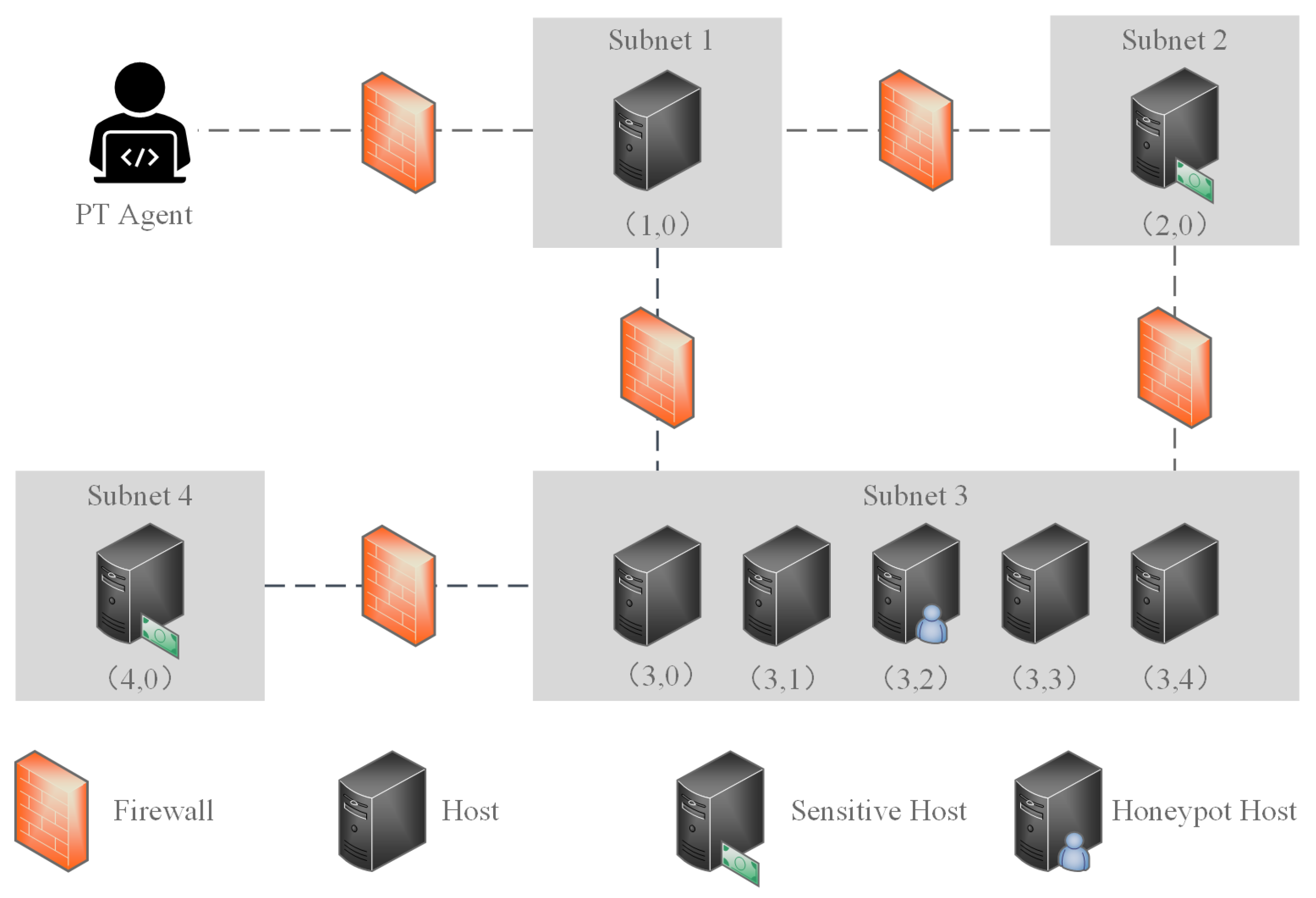
Figure 2.
PO-IPPD Framework.
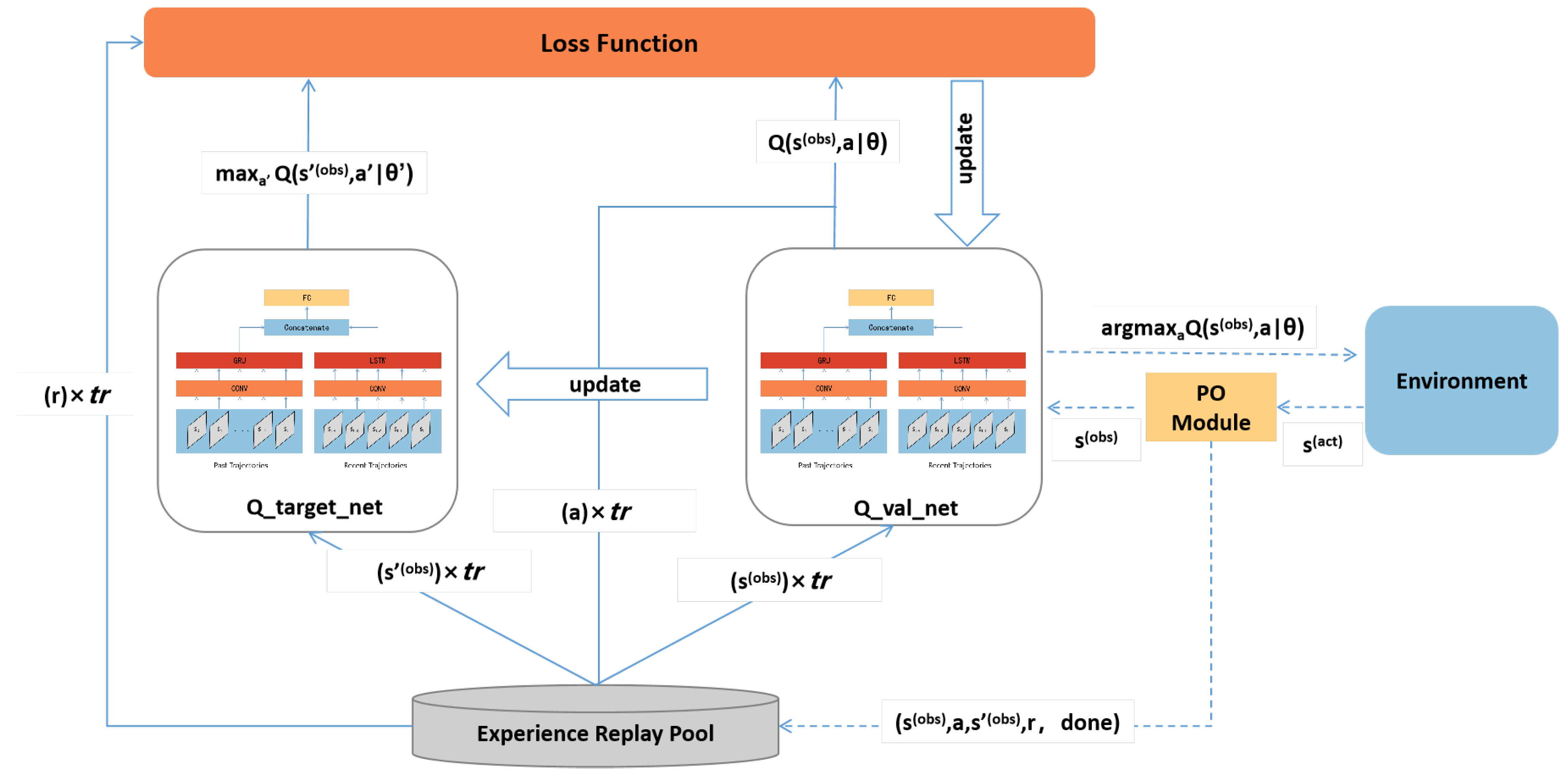
Figure 3.
PO-IPPD Network Structure.
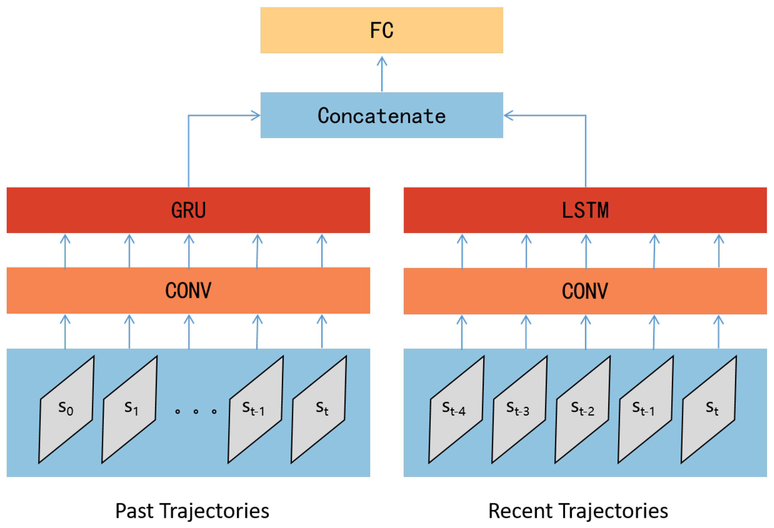
Figure 4.
Variation of Reward with Training.
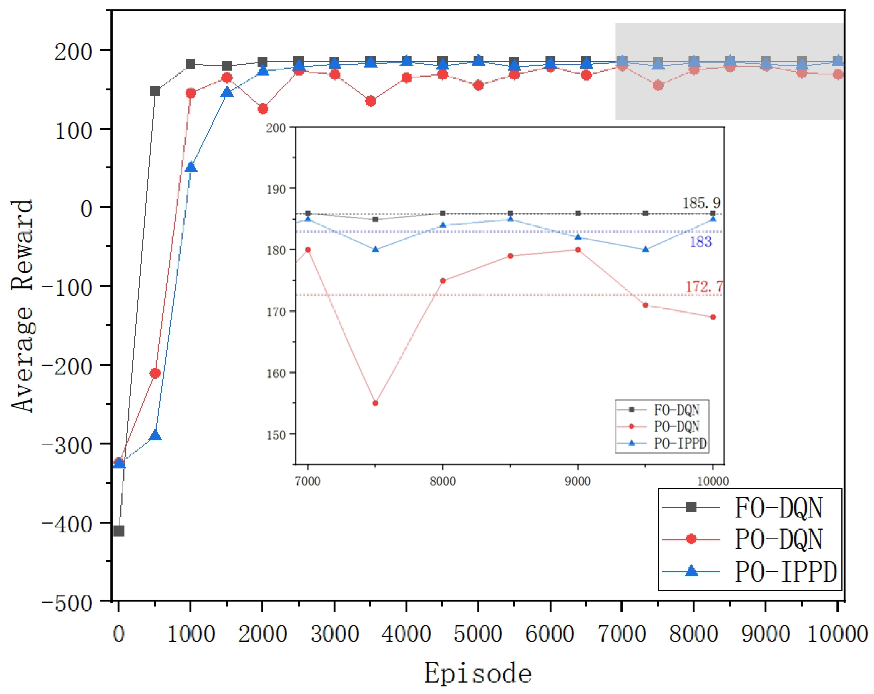
Figure 5.
Variation of Steps with Training.
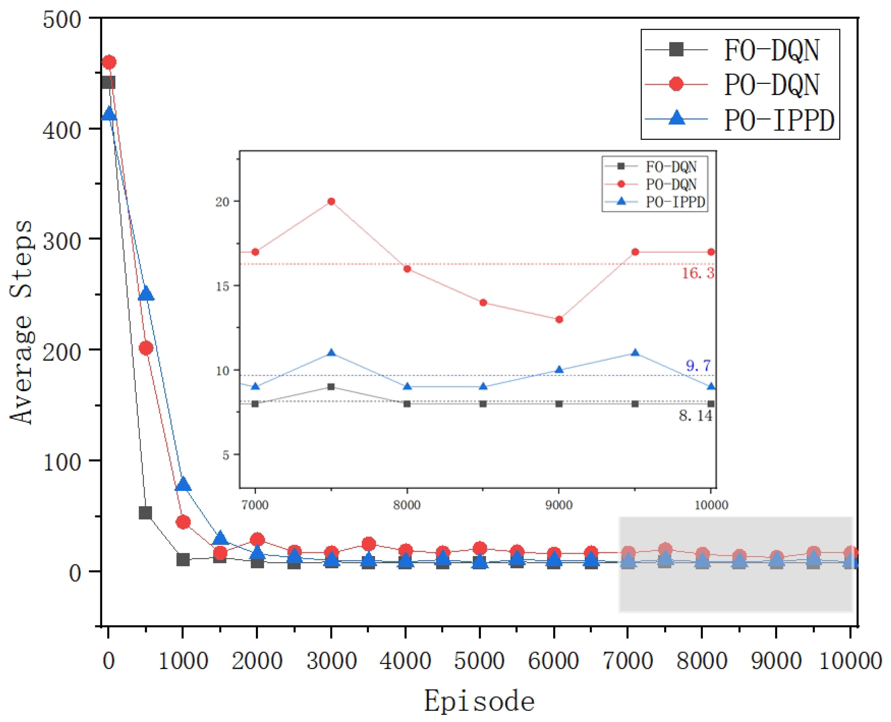
Figure 6.
Variation of (Reward/Step) with Training.
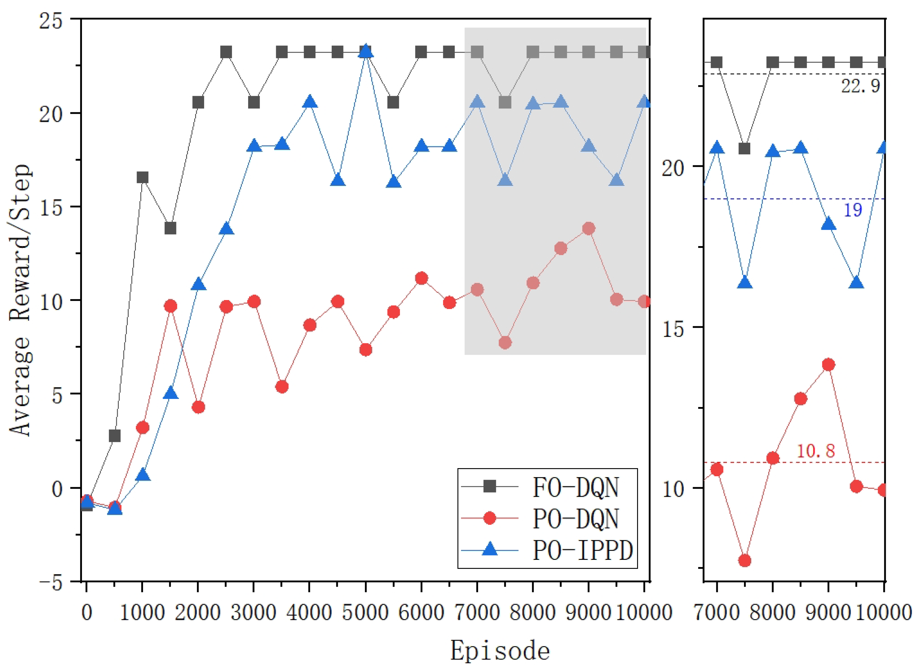
Figure 7.
Variation of (Reward) in Comparative Scenarios.


Table 1.
Hosts configuration in Figure 1.
Table 1.
Hosts configuration in Figure 1.
| Host | OS | Service | Process |
|---|---|---|---|
| (1,0) | Linux | HTTP | — |
| (2,0) (4,0) | Linux | SSH,FTP | Tomcat |
| (3,0) (3,3) | Windows | FTP | — |
| (3,1) (3,2) | Windows | FTP,HTTP | Daclsvc |
| (3,4) | Windows | FTP | Daclsvc |
Table 2.
Attack capabilities configuration in Figure 1.
Table 2.
Attack capabilities configuration in Figure 1.
| Type | Name | Prerequisites | Results | |||
|---|---|---|---|---|---|---|
| OS | Service | Process | Prob | Privileges | ||
| VE | E_SSH | Linux | SSH | — | 0.9 | User |
| E_FTP | Windows | FTP | — | 0.6 | User | |
| E_HTTP | — | HTTP | — | 0.9 | User | |
| PE | P_Tomcat | Linux | — | Tomcat | 1 | Root |
| P_Daclsvc | Windows | — | Daclsvc | 1 | Root | |
Table 3.
Basic Experiment Configurations.
| Type | Settings |
|---|---|
| CONV1: | |
| Kernel_size=3;Stride=1;Outchannels=16 | |
| Conv Structure | CONV2: |
| Kernel_size=3;Stride=1;Outchannels=32 | |
| AdaptiveAvgPool1d: | |
| output_size=1 | |
| GRU | Input=32;Hidden_size=64 |
| LSTM | Input=32;Hidden_size=64 |
| FC1: | |
| FC Structure | In_features:128,Out_features:64 |
| FC2: | |
| In_features:64,Out_features:action_space | |
| Learn Rate | 0.0001 |
| Batch_size | 64 |
| M.size | 100000 |
| Discount factor | 0.9 |
| Method capacity | 4-dimensions subnet field |
| 5-dominions host field |
Table 4.
Scalability Experiment Scenarios.
| Scenarios | Hosts | Subnets | Reward |
|---|---|---|---|
| Scenario 1 | 8 | 4 | 100*2 |
| Scenario 2 | 16 | 4 | 100*2 |
| Scenario 3 | 16 | 8 | 100*2 |
Disclaimer/Publisher’s Note: The statements, opinions and data contained in all publications are solely those of the individual author(s) and contributor(s) and not of MDPI and/or the editor(s). MDPI and/or the editor(s) disclaim responsibility for any injury to people or property resulting from any ideas, methods, instructions or products referred to in the content. |
© 2024 by the authors. Licensee MDPI, Basel, Switzerland. This article is an open access article distributed under the terms and conditions of the Creative Commons Attribution (CC BY) license (http://creativecommons.org/licenses/by/4.0/).
Copyright: This open access article is published under a Creative Commons CC BY 4.0 license, which permit the free download, distribution, and reuse, provided that the author and preprint are cited in any reuse.


