
Submitted:
27 November 2024
Posted:
28 November 2024
You are already at the latest version
Abstract
We develop in this paper the mathematical structure of the model proposed in previous works [1, 2]where define a vacuum at Planck scale as anetwork with a high rigidity cubic crystal structure made of one fundamental object defined as a fermionic dark mater confined in cubic cells of Planck length. This fundamental object can couple in a way that swiftly connect and disconnect cells at Planck time in one given direction. The evolution of these connections build pathways which guide mater providing the dynamic of movement.
Keywords:
Algebra
; spin
; spinor
; semi-spinior
; fermionic
; network
; fiber
; string
; Planck
; foam
1. Introduction
We point first some differences who characterize the model described in [1,2] against more common assumptions.
- In quantum field theory (QFT) we put oscillators in every point of the universe who gives a Hilbert space in which observables become operators. In the ground state of vacuum it does not oscillate unless a particle appear as exited states of field.
In this model instead, oscillators have a oscillation mode corresponding to vacuum, and store energy.
- Roger Penrose Spin Network [3] is a model based on a type of hypothetical fundamental object that interact in some direction. Each one is a “atom” of space that can be depicted with a point usually called a node, a dual of cubic cells in a certain type of grid. The grid of all of these nodes, and the connections between them, is called a spin network.
In this model [1,2]we start from a network of cubic cells to put a fundamental object on each. But differentiating from the former, this fundamental object is a new type of charge that oscillate at very high frequency between electric and magnetic states.
These charges are the generator of spin pulses. Then we don` t start from spinors but a object that generate it.
1.1. Precedent
In [1] we demonstrate that is feasible to reintroduce a substrate - the “ether” - and find a sub algebra of Poincaré at Planck scale to describe the dynamic of a fermion and a boson showing that the movement is Lorentz invariant. Then apply this invariance to larger objects like a interferometer and find an alternative representation to Minkowski diagram where everything is always in a particular place at a corresponding time, but have to renounce using time as a extra dimension.
In [2] we introduce a fundamental object; a fermionic structure at Planck scale that generate the vacuum and show that space look very different at Planck length scale than at atomic scale. We find there a model of Quantum Gravity (QG) where space at Planck scale must be described in a kind of Kaluza-Klein equation in . But this term in the sense of [2] is not an extra dimension in but the compaction of the other two.
2. Model Formulation
We start from a quantum state of vacuum that have no prescribed geometry.
It can be depicted by a foam of bubbles of overlapped spheres with diameter , where is the Planck length. (Figure 1)
Every bubble hold a fermionic structure we define as a “q fermion” confined in a cubic cell of side.
We will define now this q fermion in a more precise way.
This q fermion is defined as a semi spinor that oscillate at Planck frequency at one direction between both opposite faces normal to one axis. [5].
In the quantum state the direction were not defined. Every q is a sphere of diameter
To measure a state of one semi spinor makes it shows at one direction and define a axis. This measure is a perturbation that propagate to his neighbor, and makes semi spinors connect building a spinor. The image of vacuum is of cubic cell structure than a foam and this state propagate in a linear way building a chain of cubes we call a fiber [6].
In §2.1 we establish a set of postulates were this semi spinors arise as a result of a oscillation from q fermion between one electric and one magnetic state. We call “charges” these electric and magnetic states of the q fermions.
The state of q is given by the sign of rotation, spin direction and a phase factor.
In §2.2 we demonstrate that under postulates §2.1, semi spinors from cubic cells with the same chirality build spinors running up or down at speed over ultramicroscopic fibers made of a chain of cubes coupling by their spin faces with orthogonal electric, magnetic states over the other faces (Figure 2).
A spin network arise as a sum of semi spinors, that is a vector field as a sum of semi vectors. [4].
In turn, one electric/magnetic ultra short force make cells of same chirality glue fibers in a way that group in wide strings.
We identify here two direction of q; spin and electromagnetic. It belongs to different vacuum; the vacuum field of EM , and the vacuum field of space making a total of dimension plus time.
Then, electric / magnetic states will not be part of vacuum which be developed in this paper; q can be split up as:
It follow that at Planck scale the dynamic of semi spinors must be described by in . The electric and magnetic connection from over the plane normal to fibers make it group in a bundle of fibers we call “string”. But does not belong to physical space we use to describe movement.
Those strings have arbitrary directions, then it grant some orders of magnitude over Plank length scale space recover and we can use this cosmic strings to describe movement by geodesics. But with additional features. One of them is due to the fleeting connections in both electromagnetic and spinorial direction space does not complies Hausdorff postulate. Every cell is a chart, and the closed set of charts make a Atlas where the spinorial state of fibers is a sub space that overlap with the electromagnetic plane normal to fibers. Then and tensors belong to different subspaces allowing unified EM with GR.
In this paper we will focus in the spinorial state of q in a ultramicroscopic zone of a single fiber.
2.1. The Postulates
First
We start from a semi classical model, the one that have a prescribed geometry of cubes of -side (see Figure 1 and Figure 2). Every cube is a chart and a complete set of charts describe a Riemannian geometry.
We can then chose a Cartesian rectangular coordinate (t,x,y,z) in the system of a small region of this ultramicroscopic charts and put a q fermion in every cube.
It will be labeled over the z-axis with natural numbers,
Choosing we identify a single element that occupied a single cell.
If the charge contained in this cell is oriented in the plane it can be described by the equations; 1
where is the charge of the electron, is a magnetic charge, is of the order of Planck frequency [2], and a phase factor characteristic of that cell.
The transverse section of is :
It represent a electric and magnetic flux which keep the role of the generator of the electromagnetic field.
Second
There is a coupling between and that generate a new entity given by
where being the fine structure constant.
Replacing (2) and (3) in (5);
And replacing by the Planck charge in Gaussian units , the parallel component of can be expressed as a semi spinor: [6]
Third
When the electric semi vector prevails over the magnetic one, q is located over one of the z faces of the cube that we will call E. The state of q is (E) and is the semi spinor as shown in Figure 2.
When the magnetic semi vector prevails over the electric one, it is located on the opposite face that we will call M. The state of q is (M) and is the semi spinor as shown in Figure 2. The q fermion then alternate their position between face E and M of the cube over the z axis, and the orientation is given by the sign of spin; (U) if pointing up and (D) if pointing down.
Expressing the state of q as a function of the face were the semi vector is located and on its orientation, we say that the q fermion is in the state (UE), (UM), (DM), (DE) (see Figure 3).
Forth
When 2 contiguous q fermions of same chirality share a face semi vectors coupled and build a vector. We represent it as in Figure 2 - left.
A consequence is that if the spin of is oriented on the z-axis will also be and , and it perform a one dimension vector field of spinors as a fiber over z axis[9].
Because each q fermion is a semi multi vector, is half of a spinor, that is a semi spinor.
Fifth
There is a strong magnetic force of z fibers that make q fermions of same chirality glue cells creating a rigid structure of electric and magnetic monopoles over the plane.
Then z fibers were grouped in a handful making up wide cosmic strings were the cross-section over plane results in an extra dimension over the string.
We can then neglect this extra dimension and derive the dynamic of over the z axis from .
By the first and third postulates, if the monopole from is oriented in the direction, the monopole does so in the direction.
We look for the subgroup of semi-spinors from the set of contiguous elements labeled with Eq. (1) that makes possible a propagation of a spin pulse in the z direction.
We will derive the parallel component of a set of q fermions in an ultramicroscopic zone where only find semi-spinors in the z direction, then we will work in .
The forth postulate condition are given when the parallel component of of adjacent fermion share the same E/M or M/E face and U or D orientation. That is;
were is the Planck time . The factor is added to label each semi-spinor states (UE), (UM), (DM), (DE) using integer units of in which it remain in the same state in the interval (see Figure 4 and eq. (2), (3))
We will look for the conditions under adjacent semi-spinors couple building a set of spinors that perform a discrete vector field confined in a single fiber over z axis.
In this case we can replace (7), (8) in (6), and at Planck scale we get semi spinors that can be described by the equation;
Equation (9) turn a periodic function with period in which the semi-spinors remains on each face E or M during an interval in which alternate the direction U and D.
2.2. The Dynamic of Semi Spinors
We can use (9) to develop the dynamic of a single m=0 semi spinor with evaluated at .
The expression of the semi-spinor is:
and remain in the same state during the interval .
To see in which state this semi spinor is we must evaluate eq. (2), (3) at with m= 0,1,2,3 .
The values of for and are;
and remain in the state (UE) in the interval
and remain in the state (UM) in the interval
and remain in the state (DM) in the interval
and remain in the state (DE) in the interval
The 4 states for the semi-spinor evolves as (UE), (UM), (DM), (DE) and are schematic represented counterclock wise in Figure 4.
Note: The diagonals indicate the instant in which the semi-spinor reaches the opposite face and changes its location. The axis indicate the instant in which the semi-spinor is canceled and changes its direction. When the module of electric charge prevails over the magnetic one, the semi-spinor is located on the E side, and on the M side when the magnetic charge predominates.
We note with U the state with positive sign of semi-spinor and D for the negative one, but the state UE at t = 0 is made by , while at is made by . We need two cycles for the spinor to return to the original state. The time evolution for is shown.
3. A Toy Model for Spinors
Since we are not interested in the dynamics of such semi spinor but the way this media can propagate a spin pulse, we go to evaluate how it can be transported along z axis.
Then, instead of evaluating the time evolution of a single semi-spinor with at we use (9) to evaluate m semi-spinors at ; . Doing in eq. (9):
with k= 0,1,2,3, , and is enough to consider a system of 4 correlatives semi-spinors
a) For and
The state of a set of 4 semi-spinors , k=0,1,2,3 evaluated at from the interval are indicated between parentheses:
(UE)
(UM)
(DM)
(DE)
By the forth postulate, coupling happen only when a pair of semi-spinors share the same face. It also depend on the order given by the value of k, since not all adjacent semi-spinors share a face and sum to propagate a pulse.2
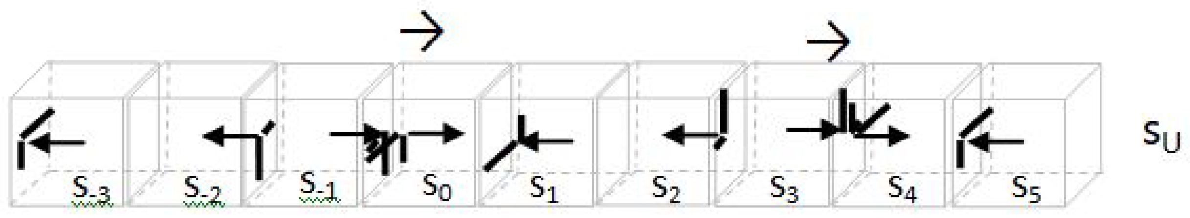
The only cells that interact and allow semi spinors to made up a spinor are 4n+3 and 4n+2 3
The sum of two adjacent semi-spinors in state DE/DM gives rise to a spinor down as a sum vector [5].
Using :
We observe in (9) that for and :
and the sum vector represents an infinite series of spin pulses down equidistant in that never cancel and move one cell down over the fiber with velocity .
Taking a set of 4 cells to consider the spinor only as a sum of the two semi spinors that form it, we define the unit
To pass to the continuum, multiply and divide by c the first member and by the second. Replacing in (7) for taking both directions and ,
=
To consider the finite width of this pulse we introduce the function H.
which take the value 1 in the interval
and is null outside.
We name this spinor pulse, and agree to indicate the spin state from eq. (9) as the sum of 2 semi vector by placing the subscript of the empty cell first.
and neglect the internal oscillations of the cells of the fiber in which the fermions do not interact in the z direction because this oscillation do not represent anything physical.4
Taking one out of every 4 cells we can eliminate k in (11) and take from (1) for an infinite number of pulses that never cancel.
The complete expression of a train of pulses on a fiber with and finally is
were H take the sign of the argument.
b) For and
For the negative sign of m, the Equation (9) in terms of n,k:
satisfies and represents a pulse traveling up over the z axis.
The state of 4 consecutive semi-spinors evaluated in the interval are indicated between parenthesis;
(UM)
(UE)
(DE)
(DM)
Figure 6.
fiber.
Coupling only take place between the UM/UE pair of semi-spinors. The only cells that allow us to be added is for U semi-spinors and .5 The complete expression of this spin pulses on a U fiber is
We can get two more expressions for the negative sign of . There were two more type of fibers with :
c) and
(UE)
(UM)
(DM)
(DE)
The only cells we can sum are 4n+2 and 4n+3 and represents a pulse D that moves inside the z fibes in the positive direction:
We indicate these spin pulses with negative time arrow as [12];
d) and
For the negative sign of n, the spinorial components that allow interact are 4n-1 and 4n, and represents a U pulse that move down over the z axis. We indicate these spin pulses inside a z fiber with negative time arrow as
We can get rid from H by observing in (15-18) that H limits the no null spin value to the interval in which this is a distribution centered on .
To demonstrate that the parallel component of q build up a spinor, we integrate a single pulse from eq. (15) in the interval :
Then q is the generator of a spin pulse inside each one of the four types of fibers.
Disregarding the pulse width of the spinors, we can replace by .
Expressions (15-18) can be summarized in 4 type of spinor’s fibers:
4. Spin Foam, Spin Network, Fibers and Strings
Eq. (19) to (22) express one eigenstate of the spin foam. They are the exact description of space time and can be generalized to describe the dynamics of particles with strings and fibers.
We should see vacuum as a spin foam in which identify strings made up of , , and fibers. Vacuum have strings immersed in a spin foam of bubbles, each one occupied by a q fermion.
Observable determine a direction, and bubbles become cubes; a prescribed geometry arise as cosmic strings.
This model match well with Veneziano explanation of Regge trajectories [14] for the total spin of the system . Inside strings, fibers of opposite chirallity alternate and .
But we can combine this four classes of fibers to build up a perturb over the normal mode of oscillation. It will be a observable which spin can take values [3]:
is a perturb over , or , fibers.
is a perturb over , , or , , fibers.
.....
each of them have a physical meaning.
We can exemplify by describing a photon that travels to as a perturb between + fibers, while another traveling to requires + fibers.
5. Summary
We start from a quantum state of vacuum as a spin foam of spheres of diameter in which we can not ascribe a direction of spin or charges.
A eigenstate of cubic cells of side give us a semi classic mechanics in which space is still quantified holding a multi semi vector of electric, magnetic and spin split up in a parallel and normal semi vector spaces, but with a geometry and coordinates over each vector space.
We use the parallel sub space to sketch a toy model who describe a set of semi spinor who build a spinor and its dynamic. Then fund a group of equations (19) to (22) that describe the dynamic of a single spinor inside a fiber.
We develop this mathematics equations as a pending issue of the model developed in the previous papers in which had used these equations to describe the vacuum state at Planck scale by a spin network in which we identify fibers, strings and branes in algebraic terms of the natural coordinates of eq. (1).
- In [1] we demonstrate that this network is Lorentz invariant: Bosons and fermions are both perturb of this media that travel toward the fibers and show the reality in a new type of diagram over one Euclidean plane instead the Minkowski’ s.
We show there that this loops involve fibers that give raise a sub algebra of Poincare that recover Lorentz metric and also demonstrate there with the help of frames that everything is always in a particular place at a corresponding time.
- in [2] we suggest that energy is a kind of hole, deficit or vacancy of spin pulses in the coordinator field. It was seen there that fermions with negative charge are loops of holes inside fibers while fermions with positive charge comes from a loop of holes inside fibers.
Also in [2] use this model to explain gravity as a special case of string theory and apply it to relate the inertial and gravitational mass as a unique entity, and show how inertial field store and feed energy.
While electromagnetism arise as interaction between fibers, and because strings have no null section, we can use this model to include electroweak and strong forces on it.
References
- Daniel Levi and Daniel B. Berdichevsky; “About a Lorentz invariant aether and a alternative view to Minkowski diagram”, https://medcraveonline.com/AAOAJ/AAOAJ-07-00166.pdf.
- Daniel Levi; “A string theoty of Quantum Gravity and inertial fields for the description of reality”. Preprints.org, ID 77591.
- Roger Penrose Quantum Theory and Beyond, ed. T. Bastin, Cambridge University Press, Cambridge, 1971, pp. 151–180.
- Semi-vectors and spinors. By A. Einstein and W. Mayer. (Received on 10 November 1932).
- Brett McInnes, The Semispin Groups in String Theory, J. Math. Phys. 40:4699-4712, 1999 (arXiv:hep-th/9906059).
- A bound for canonical dimension of the (semi-)spinor groups. Duke Math. J. 133 (2006), no. 2, 391–404. Nikita A. Karpenko. [CrossRef]
- Annales de la Fondation Louis de Broglie, Volume 12, no.4, 1987.
- Dirac’s aether in relativistic quantum mechanics, Bibcode:1983FoPh...13..253P. [CrossRef]
- Vector-fermion dark mater, arxiv.org/pdf/1804.10289.pdf.
- Einstein, 1956, p 165f, Generalization of Gravitation Theory, Relativistic theory, Apendix II.
- arxiv.org/pdf/hep-ph/9810365v1.pdf, The status of CPT, V. Alan Kostelecky, October 1998.
- Greaves, H. (2007). Towards a geometrical understanding of the CPT theorem.
- arXiv : 1101:5061 v1 The spin foam network for Quantum Gravity.
- Veneziano, G. (1968), Nuovo Cimento, 57A, 190.
- Cherkas and Kalashnikov, Eicheons instead of Black holes https://arxiv.org/pdf/2004.03947.pdf.
- An inhomogeneous toy model of the quantum gravity with the explicitly evolvable observables https://link.springer.com/article/10.1007/s10714-012-1441-5.
- F. Clauser; M.A. Horne; A. Shimony; R.A. Holt (1969), “Proposed experiment to test local hidden-variable theories", Phys. Rev. Lett., 23 (15): 880–4, Bibcode:1969PhRvL..23..880C. [CrossRef]
| 1 | In [1] we must use a parameter instead t. Here we work in and use for time t in this preferred reference frame. |
| 2 | See Figure 3
|
| 3 | Only (DM) and (DE) share face. |
| 4 | We can demonstrate that during this intervals they interact in the xy plane building charged membranes that let polarization of vacuum and are the generator of the electromagnetic field. |
| 5 | To see this rearrange the 4 states in Figure 3 (UM), (UE), (DE), (DM) |
Figure 1.
A quantum image of space is a spin foam. When a spin direction is prescribed, a description of cubes is preferred.
Figure 1.
A quantum image of space is a spin foam. When a spin direction is prescribed, a description of cubes is preferred.
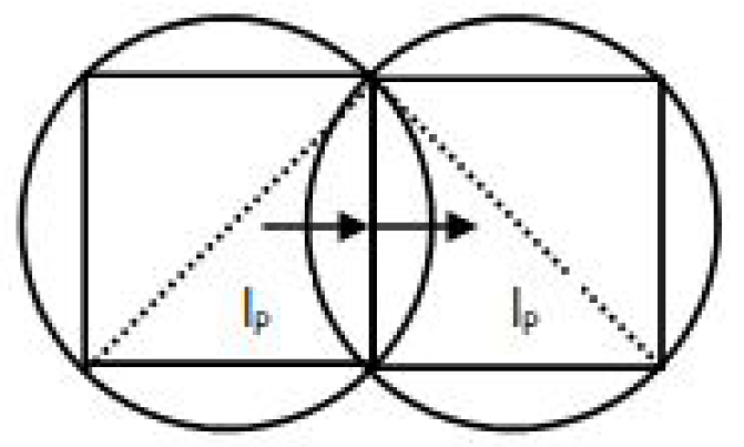
Figure 2.
Right; semi spinors over M face and over E face. Electric charge over x axis and magnetic charge over y axis.
Left; a spinor over the z axis as a sum
Figure 2.
Right; semi spinors over M face and over E face. Electric charge over x axis and magnetic charge over y axis.
Left; a spinor over the z axis as a sum
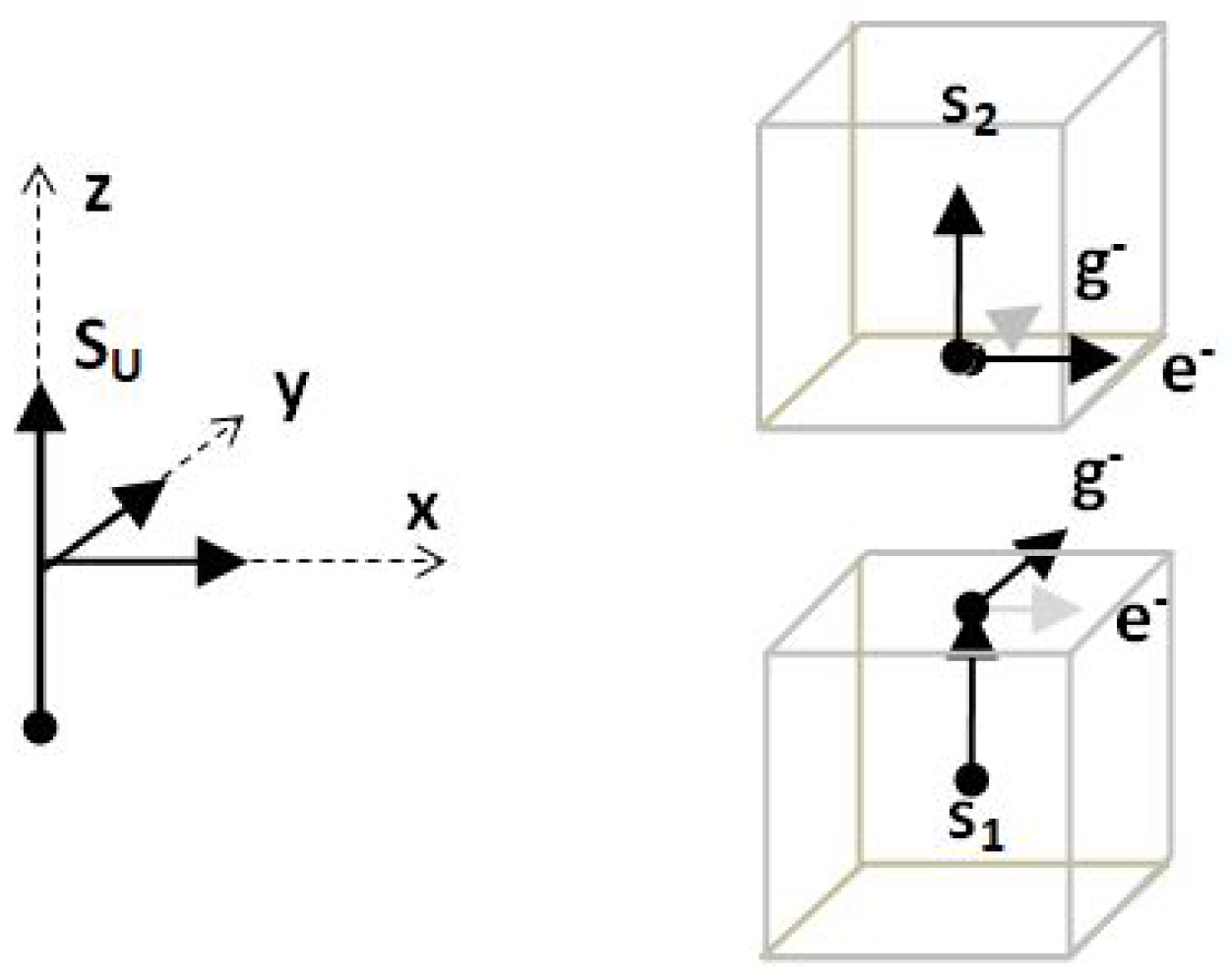
Figure 3.
Rep. of 4 states or over the z axis, here building spinor as a sum of DE + DM.
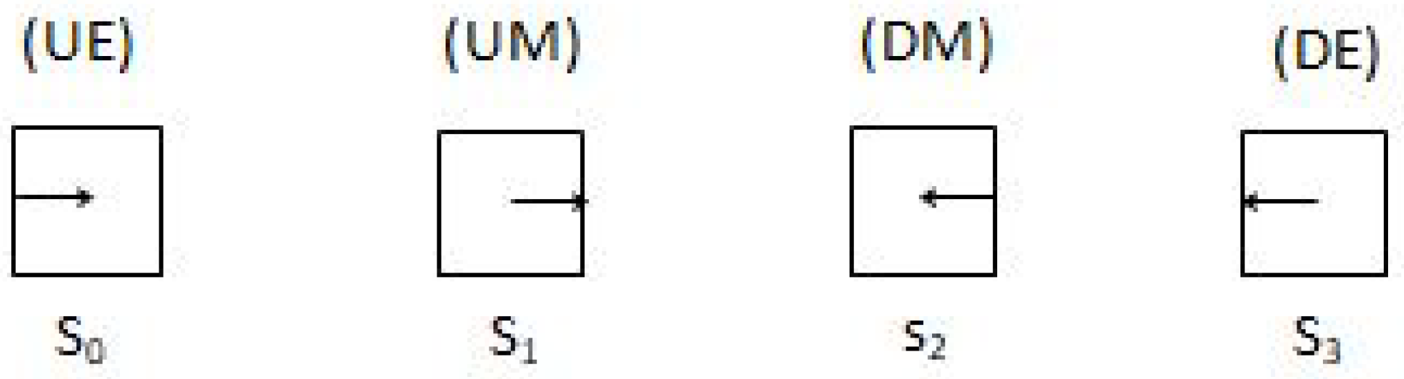
Figure 4.
Because the factor in , the state in eq. (9) at time , is in the middle of the interval .
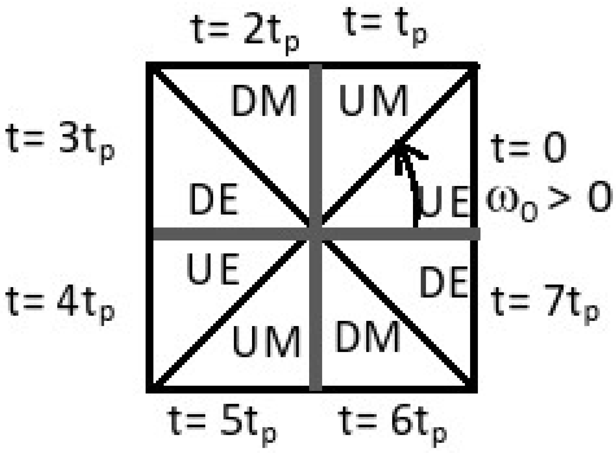
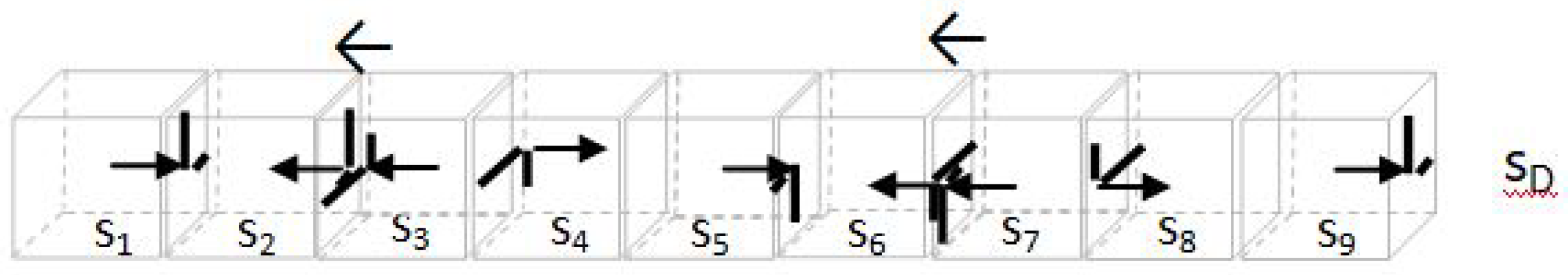
Figure 5.
fiber.
Disclaimer/Publisher’s Note: The statements, opinions and data contained in all publications are solely those of the individual author(s) and contributor(s) and not of MDPI and/or the editor(s). MDPI and/or the editor(s) disclaim responsibility for any injury to people or property resulting from any ideas, methods, instructions or products referred to in the content. |
© 2024 by the authors. Licensee MDPI, Basel, Switzerland. This article is an open access article distributed under the terms and conditions of the Creative Commons Attribution (CC BY) license (http://creativecommons.org/licenses/by/4.0/).
Copyright: This open access article is published under a Creative Commons CC BY 4.0 license, which permit the free download, distribution, and reuse, provided that the author and preprint are cited in any reuse.


