Submitted:
09 November 2024
Posted:
11 November 2024
You are already at the latest version
Abstract
We study a duel game in which each player has partial knowledge of the game parameters. We present a method by which, in the course of repeated plays, each player estimates the missing parameters and consequently learns his optimal strategy.
Keywords:
Duel game
; tree game
; backward induction
; learning
Introduction
We study a duel game in which certain game parameters (related to the players’ kill probabilities) are unknown and present a method by which each player can estimate the opponent’s parameters and consequently learn his optimal strategy.
The duel game with which we are concerned has been presented in [1] and a similar one in [2]. The game is a variation of duels and, more generally, games of timing studied in the literature [3,4,5].
The paper is organized as follows. In Section 1 we present the rules of the game. In Section 2 we solve the game under the assumption of complete information. In Section 3 we present an algorithm for solving the game when the players have incomplete information. In Section 4 we evaluate the algorithm by numerical experiments. Finally, in Section 5 we summarize our results and present our conclusions.
1. Game Description
The duel with which we are concerned is played between players and , under the following rules.
- It is played in discrete rounds (time steps) .
- In the first turn, the players are at distance D.
- (resp. ) plays on odd (resp. even) rounds.
- On his turn, each player has two choices: (i) he can shoot his opponent or (ii) he can move one step forward, reducing their distance by one.
- If shoots, he has a kill probability of hitting (and killing) his opponent, where d is their current distance. If he misses, the opponent can walk right next to him and shoot him for a certain kill.
- Each player’s payoff is 1 if he kills the opponent and if he shoots and misses (in which case he is certain to be killed).
For , we will denote by the position of at round t. The starting positions are and , with . The distance between the players at time t is
For , the kill probability is a decreasing function with . It is convenient to describe the kill probabilities as vectors:
This duel can be modeled as an extensive form game or tree game. The game tree is a directed graph with vertex set
where
- the vertex corresponds to a game state in which the players are at distance d and
- the vertex is a terminal vertex, in which the “active” player has fired at his opponent.
The edges correspond to state transitions; it is easy to see that the edge set is
An example of the game tree, for , appears in Figure 1. The circular (resp. square) vertices are the ones in which (resp. ) is active and the rhombic vertices are the terminal ones.
To complete the description of the game, we will define the expected payoff for the terminal vertices. Note that the terminal vertex is the child of the nonterminal vertex d in which:
- The distance of the players is d and, assuming to be the active player, his probability of hitting his opponent is .
- The active player is (resp. ) iff d is even (resp. odd).
Keeping the above in mind, we see that the payoff (to ) of vertex is
The payoff to at vertex is . This completes the description of the duel.
2. Solution with Complete Information
It is easy to solve the above duel when each player knows D and both and . We construct the game tree as described in Section 1 and we solve it by backward induction. Since the method is standard, we simply give an example of its application. Suppose that
We take , , , . The kill probabilities are
The game tree with terminal payoffs is illustrated in Figure 2.
By the standard backward induction procedure we select the optimal action at each vertex and also compute the values of the nonterminal vertices. These are indicated in Figure 3 (optimal actions correspond to thick edges). We see that the game value is , attained by shooting when the players are at distance 3 (which happens in round 4).
We next present a proposition which characterizes each player’s optimal strategy in terms of a shooting threshold. 1 In the following we use the standard notation by which “” denotes the “other player”. I.e., and .2
Theorem 1.
We define for the shooting criterion vectors where
Then the optimal strategy for is to shoot as soon as it is his turn and the distance of the players is less than or equal to the shooting threshold , where:
Proof.
Suppose the players are at distance d and the active player is .
- If will not shoot in the next round, when their distance will be , then must also not shoot in the current round, because he will have a higher kill probability in his next turn, when they will be at distance .
- If will shoot in the next round, when their distance will be , then should shoot iff (his kill probability now) is higher then (’s miss probability in the next round). In other words, must shoot iffor, equivalently, iff
Hence we can reason as follows.
- At vertex 1, is active and his only choice is to shoot.
-
At vertex 2, is active and he knows will certainly shoot in the next round. Hence will shoot iff he has an advantage, i.e., iffThis is equivalent to and will always be true.
- Hence at vertex 3, is active and he knows that will certainly shoot in the next round (at vertex d). So will shoot iffwhich is equivalent to . Also, if , then will know, when the game is at vertex 4, that will not shoot when at 3. So, will not shoot when at 4. But then, when at 5, knows that will not shoot when at 4. Continuing in this manner we see that implies that firing will take place exactly at the vertex 2.
- On the other hand, if , then knows when at 4 that will shoot at the next round. So, when at 4, should shoot iff . If, on the other hand, , then will not shoot when at 4 and will shoot when at 3.
- We continue in this manner for increasing values of d. Since both and are decreasing with d, there will exist a maximum value (it could equal D) in which some will be greater than one and will be active; then must shoot as soon as the game reaches or passes vertex and he “has the action”.
This completes the proof. □
Returning to our previous example, we compute the vectors for and list them in the following table.

Table 2.
Shooting Criterion
| d | 1 | 2 | 3 | 4 | 5 | 6 |
|---|---|---|---|---|---|---|
| Round | 6 | 5 | 4 | 3 | 2 | 1 |
| 1.500 | 1.040 | 0.827 | 0.700 | 0.614 | ||
| 1.707 | 1.077 | 0.833 | 0.697 | 0.608 |
For the shooting criterion is last satisfied when the distance is ; this happens at round 4 in which is inactive, so he should shoot at round 5. However, for the shooting criterion is also last satisfied at distance and round 4, in which is active; so he should shoot at round 4. This is the same result we obtained with backward induction.
3. Solution with Incomplete Information
We will now present an approach to the solution of the duel when each player has incomplete knowledge of his opponent’s kill probability function. More specifically, we assume that the players’s kill probabilities have, for all d, the form where is a parameter vector. Assuming has and has , we have
Furthermore, we assume that both players know the general form and each knows his own parameter vector but not the of his opponent.
Obviously in this case the players cannot perform the computations of either backward induction or the shooting criterion. Consequently we will propose an “exploration-and-exploitation” approach. In other words, under the assumption that multiple duels will be played, each player initially adopts a random strategy and, collecting information from played games, he gradually builds and refines an estimate of his optimal strategy.
We give now a more detailed description of our approach, by Algorithm 1, presented below in pseudocode.
| Algorithm 1:Learning the Optimal Duel Strategy |
|
The following remarks explain the operation of the algorithm.
- In line 1 the algorithm takes as input: (i) the duel parameters D, , , (ii) two learning parameters and (iii) the number R of duels used in the learning process.
-
Then, in lines 2-3, the true kill probability (for ) is computed by the function CompKillProb, which simply computesWe emphasize that these are the true kill probabilities.
- In line 4 initial, randomly selected parameter vector estimates are generated.
-
Then the algorithm enters the loop of lines 5-15 (executed for R iterations) which constitutes the main learning process.
- (a)
-
In lines 6-7 we compute new estimates of the kill probabilities , by function CompKillProb, based on the estimates of parameters :We emphasize that these are estimates of the kill probabilities, based on the parameter estimates .
- (b)
- In lines 8-9 we compute new estimates of the shooting thresholds , by function CompShootDist. For , this is achieved by computing the shooting criterion using the (known to ) and the (estimated by ) .
- (c)
- In line 10, (which will be used as a standard deviation parameter) is divided by the factor .
- (d)
-
In line 11 the result of the duel is computed by the function PlayDuel. This is achieved as follows:
- For , selects a random shooting distance from the discrete normal distribution [6] with mean and standard deviation .
- With both selected, it is clear which player will shoot first; the outcome of the shot (hit or miss) is a Bernoulli random variable with success probability , where is the shooting player. Note that is the true kill probability.
The result is stored in a table X, which contains the data (shooting distance, shooting player, hit or miss) of every duel played up to the r-th iteration. - (e)
- In line 12, the entire game records X are used by EstKillProb to obtain empirical estimates of the kill probabilities . These estimates are as follows:where
- (f)
- In line 13-14 the function EstPars uses a least squares algorithm to find (only for the who currently has the action) values which minimize the squared error
- (g)
- In line 21 the algorithm returns the final estimates of optimal shooting distances and parameters .
Note that multiplication by results in . Hence, while in the initial iterations of the learning process the players essentially use random shooting thresholds (exploration) with standard deviation , it is hoped that, as r increases and of the used shooting thresholds goes to zero, the estimates of the kill probabilities and shooting thresholds will converge to their optimal values (exploitation). This is actually corroborated by the experiments we present in the next section.
4. Experiments
In this section we present numerical experiments to evaluate our approach.
4.1. Experiments Setup
In the following subsection we present several experiment groups, all of which share the same structure. Each experiment group corresponds to a particular form of the kill probability functions. In each case, the kill probability parameters, along with the initial player distance D, are the game parameters. For each choice of game parameters we proceed as follows.
First we select the learning parameters and the number of learning steps R. These, together with the game parameters, are the experiment parameters. Then we select a number J of estimation experiments to run for each choice of experiment parameters. For each of the J experiments we compute the following quantities.
- The relative error of the final kill probability parameter estimates. For a given parameter , this error is defined to be
- The relative error of the shooting threshold estimates. Letting be the estimate of the shooting threshold based on the true kill probability vector and kill probability vector estimate , this error is defined to be
-
The relative error of the optimal payoff estimates. Letting be the estimate of the optimal payoff (computed from the estimated shooting thresholds ) , this error is defined to beNote that , because the game is zero-sum.
4.2. Experiment Group A
In this group the kill probability function has the form:
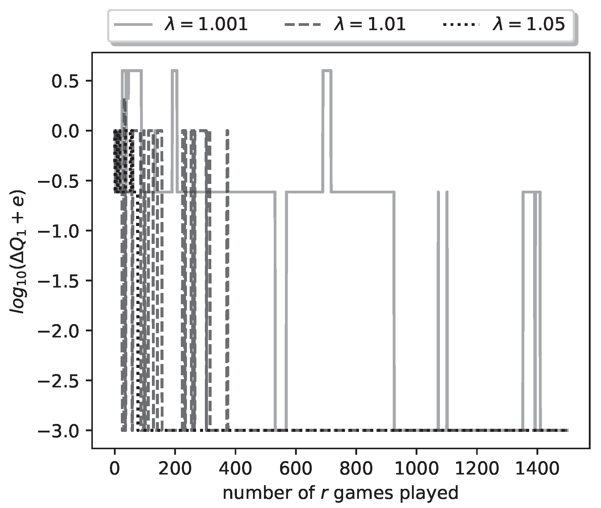
Let us look at the final results of a representative run of the learning algorithm. With , , , and , we run the learning algorithm with , and for three different values . In Figure 4 we plot the logarithm (with base 10) of the relative payoff error (we have added to deal with the logarithm of zero error). The three curves plotted correspond to the values 1.001, 1.01, 1.05. We see that, for all values, the algorithm achieves zero relative error; in other words it learns the optimal strategy for both players. Furthermore convergence is achieved by the 1500-th iteration of the algorithm (1500-th duel played), as seen by the achieved logarithm value (recall that we have added to the error, hence the true error is zero). Convergence is fastest for the largest value, i.e., , and slowest for the smallest value .
Figure 4.
Plot of logarithmic relative error of ’s payoff for a representative run of the learning process.
Figure 4.
Plot of logarithmic relative error of ’s payoff for a representative run of the learning process.
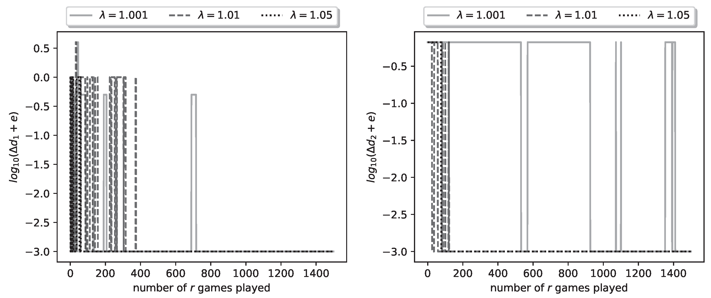
In Figure 5 we plot the logarithmic relative errors . These also, as expected, have converged to zero by the 1500-th iteration.
Figure 5.
Plot of logarithmic relative errors , for a representative run of the learning process.
The fact that the estimates of the optimal shooting thresholds and strategies achieve zero error, does not imply that the same is true of the kill probability parameter estimates. In Figure 6 we plot the relative errors , .
Figure 6.
Plot of relative parameter errors , for a representative run of the learning process.
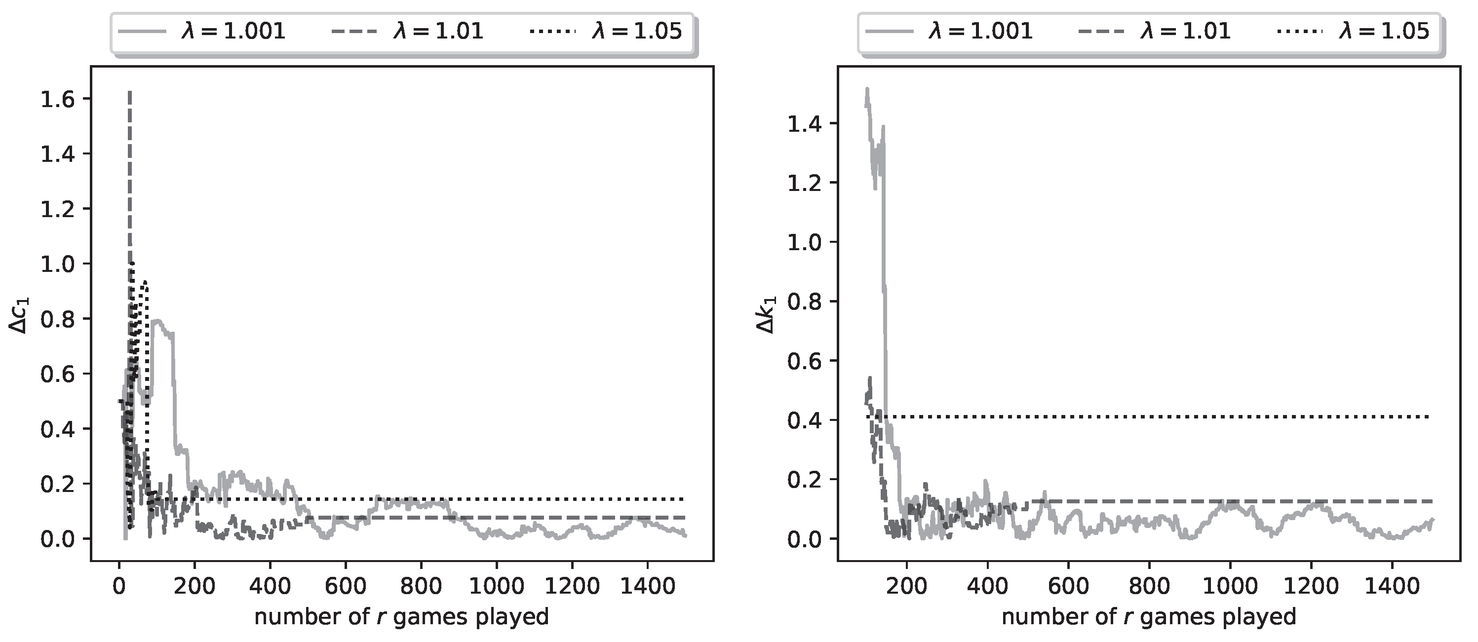
It can be seen that these errors do not converge to zero; in fact, for the errors converge to fixed nonzero values, which indicates that the algorithm obtains wrong estimates. However, the error is sufficiently small to still result in zero-error estimates of the shooting thresholds. The picture is similar for the errors , , hence their plots are omitted.
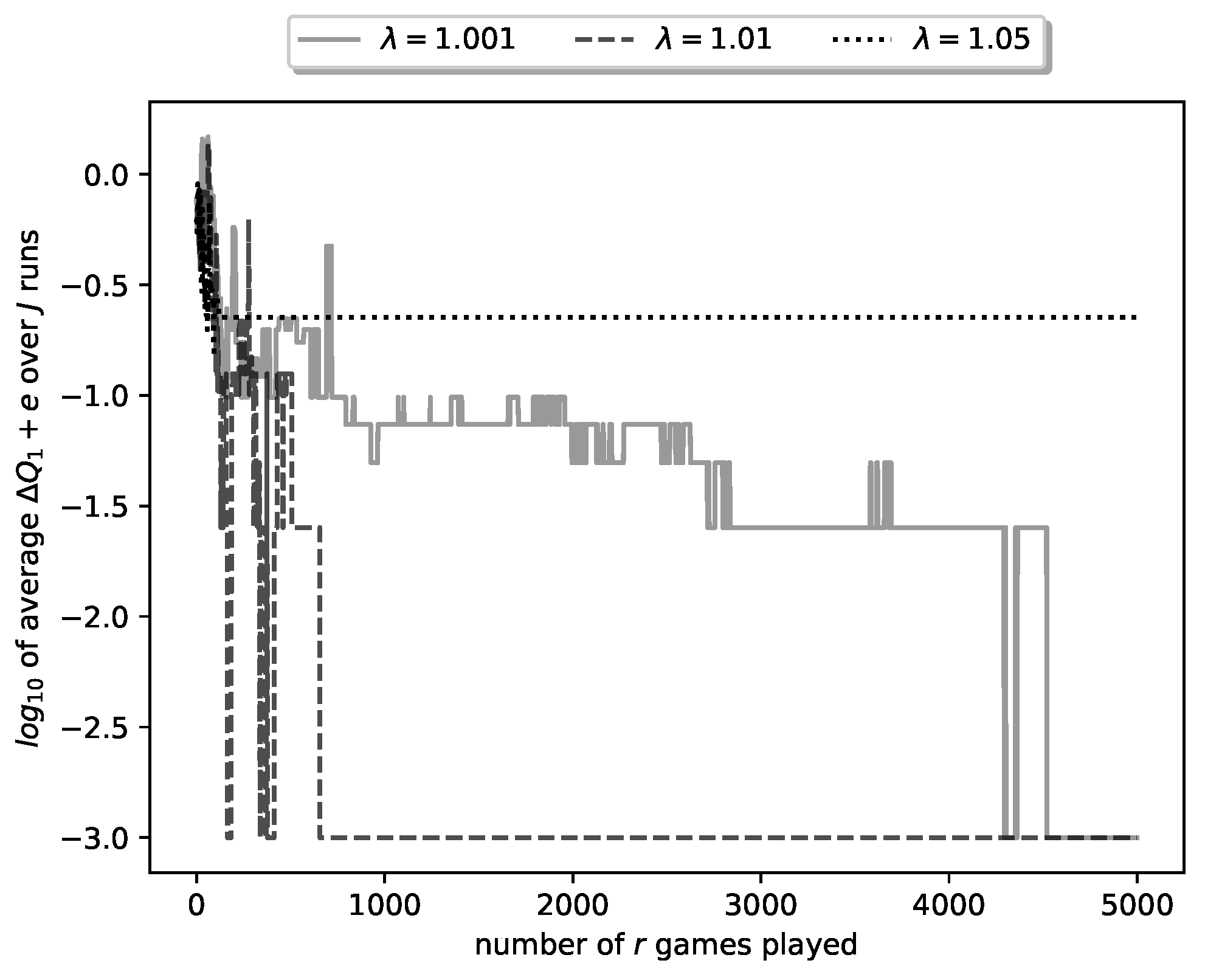
In the above we have given results for a particular run of the learning algorithm. This was a successful run, in the sense that it obtained zero-error estimates of the optimal strategies (and shooting thresholds). However, since our algorithm is stochastic, it is not guaranteed that every run will result in zero-error estimates. To better evaluate the algorithm, we have run it for times and averaged the obtained results. In particular, in Figure 7 we plot the average of ten curves of the type plotted in Figure 4. Note that now we plot the curve for plays of the duel.
Figure 7.
Plot of (’s payoff) for a representative run of the learning process.
Several observations can be made regarding Figure 7.
- For the smallest value, namely , the respective curve reaches at . This corresponds to zero average error, which means that, in some algorithm runs, it took more than 4500 iterations (duel plays) to reach zero error.
- For the , all runs of the algorithm reached zero-error after runs.
- Finally, for , the average error never reached zero; in fact 3 out of 10 runs converged to nonzero-error estimates, i.e., to non-optimal strategies.
The above observations corroborate a fact well known in the study of reinforcement learning [7]. Namely, a small learning rate (in our case small ) results in higher probability of converging to the true parameter values, but also in slower convergence. This can be explained as follows: a small results in higher values for a large proportion of duels played by the algorithm; i.e., in more extensive exploration, which however results in slower exploitation (convergence). 3
We conclude this group of experiments by running the learning algorithm for various combinations of game parameters; for each combination we record the average error attained at the end of the algorithm (i.e., at ). The results are summarized at the following tables.
Table 3.
Values of final average relative error for , and various values of , , . D is fixed at .
| 1.001 | 1.01 | 1.05 | |||||||
| 0.50 | 1.00 | 1.50 | 0.50 | 1.00 | 1.50 | 0.50 | 1.00 | 1.50 | |
| 1.00 | 0.000 | 0.000 | 0.000 | 0.000 | 0.100 | 0.482 | 0.224 | 0.500 | 1.207 |
| 1.50 | 0.000 | 0.000 | 0.000 | 0.059 | 0.049 | 1.748 | 0.215 | 0.480 | 3.777 |
| 2.00 | 0.000 | 0.000 | 0.048 | 0.074 | 0.199 | 0.097 | 0.144 | 0.980 | 0.072 |
Table 4.
Round at which converged to zero for all sessions for , and various values of , , . D is fixed at . If did not converge for all sessions we note for how many sessions it converged.
Table 4.
Round at which converged to zero for all sessions for , and various values of , , . D is fixed at . If did not converge for all sessions we note for how many sessions it converged.
| 1.001 | 1.01 | 1.05 | |||||||
| 0.50 | 1.00 | 1.50 | 0.50 | 1.00 | 1.50 | 0.50 | 1.00 | 1.50 | |
| 1.00 | 4521 | 1456 | 2983 | 656 | 9/10 | 8/10 | 7/10 | 5/10 | 5/10 |
| 1.50 | 3238 | 2939 | 1754 | 7/10 | 9/10 | 9/10 | 0/10 | 8/10 | 6/10 |
| 2.00 | 4153 | 423 | 8/10 | 2/10 | 9/10 | 6/10 | 3/10 | 4/10 | 6/10 |
From Table 6 and Table 7 we see that for almost all learning sessions conclude in zero , while increasing the value of results in more sessions concluding with non-zero error estimates. Furthermore, we observe that when the average converges to zero for multiple values of the convergence is faster for bigger . These results highlight the trade off between exploration and exploitation discussed above.
Finally, in Table 8 we see how many learning sessions were run and how many converged to zero error estimate for different values of D and .
Table 5.
Fraction of learning sessions that converged to for different values of D and .
| 1.001 | 1.01 | 1.05 | |
| D | |||
| 8 | 163/170 | 144/170 | 89/170 |
| 10 | 165/170 | 139/170 | 81/170 |
| 12 | 161/170 | 123/170 | 68/170 |
| 14 | 164/170 | 134/170 | 73/170 |
| total | 653/680 | 540/680 | 311/680 |
Table 6.
Values of final average relative error for , and various values of , , . D is fixed at .
| 1.001 | 1.01 | 1.05 | ||
| 1 | 0.000 | 0.233 | 1.000 | |
| 1 | 0.000 | 0.000 | 0.799 | |
| 1 | D | 0.800 | ||
| 0.000 | 0.000 | 2.799 | ||
| D | 0.000 | 0.000 | 0.777 | |
| D | 0.000 | 0.000 | 0.480 |
Table 7.
Round at which converged to zero for all sessions for , and various values of , , . D is fixed at . If did not converge for all sessions we note for how many sessions it converged.
Table 7.
Round at which converged to zero for all sessions for , and various values of , , . D is fixed at . If did not converge for all sessions we note for how many sessions it converged.
| 1.001 | 1.01 | 1.05 | ||
| 1 | 287 | 7/10 | 0/10 | |
| 1 | 812 | 333 | 9/10 | |
| 1 | D | 7/10 | 9/10 | 9/10 |
| 326 | 139 | 5/10 | ||
| D | 225 | 397 | 5/10 | |
| D | 711 | 464 | 6/10 |
Table 8.
Fraction of learning sessions that converged to for different values of D and .
| 1.001 | 1.01 | 1.05 | |
| D | |||
| 8 | 76/110 | 80/110 | 49/110 |
| 10 | 97/110 | 95/110 | 56/110 |
| 12 | 94/110 | 78/110 | 39/110 |
| 14 | 100/110 | 84/110 | 40/110 |
| total | 367/440 | 337/440 | 184/440 |
4.3. Experiment Group B
In this group the kill probability function is piecewise linear
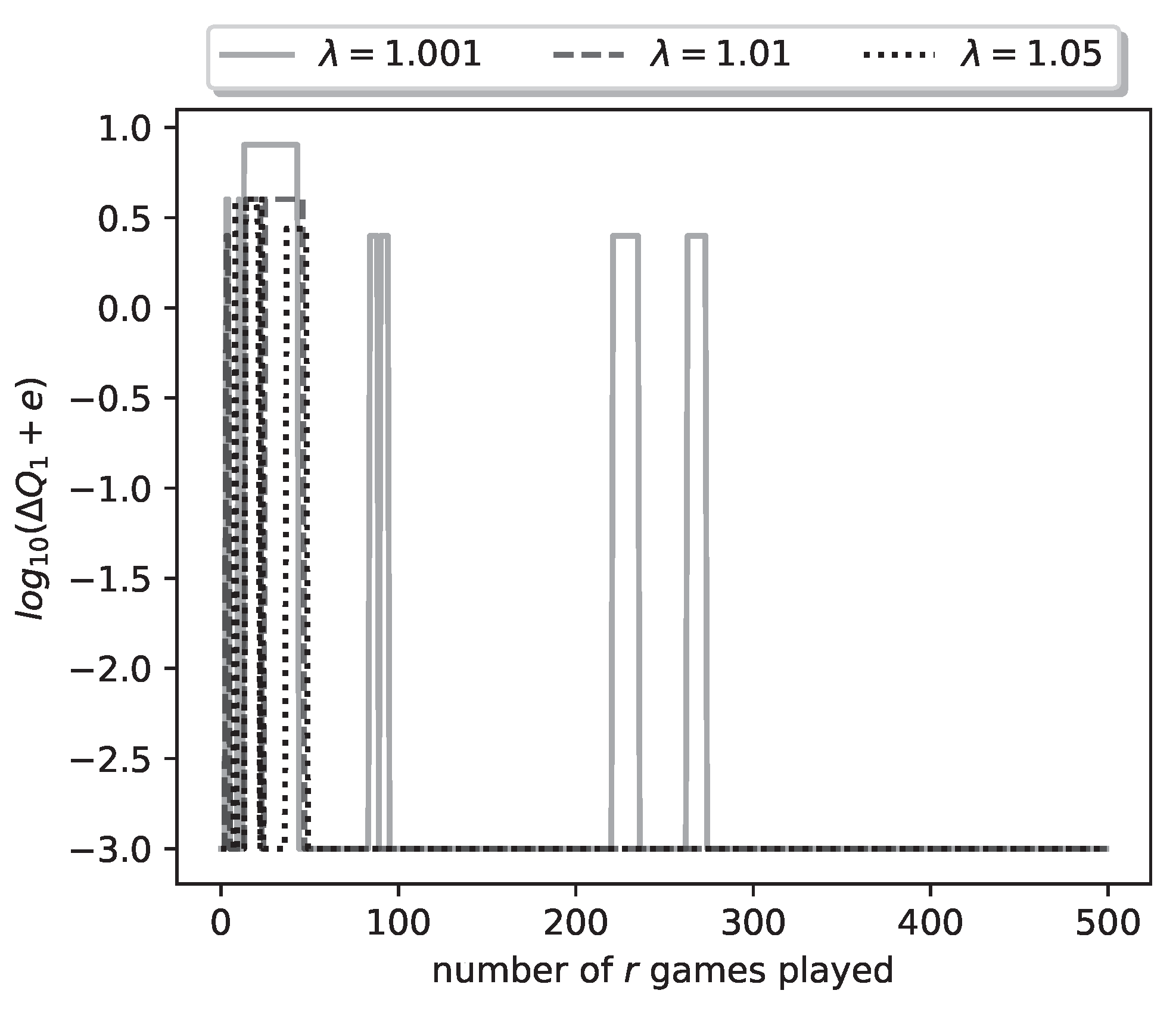
Let us look again at the final results of a representative run of the learning algorithm. With , , , and , we run the learning algorithm with , and for the values . In Figure 8 we plot the logarithm (with base 10) of the relative payoff error . We see similar results as in Group A, for all values, the algorithm achieves zero relative error. Convergence is achieved by the 300-th iteration of the algorithm and it is fastest for , and slowest for .
Figure 8.
Plot of logarithmic relative error of ’s payoff for a representative run of the learning process.
Figure 8.
Plot of logarithmic relative error of ’s payoff for a representative run of the learning process.
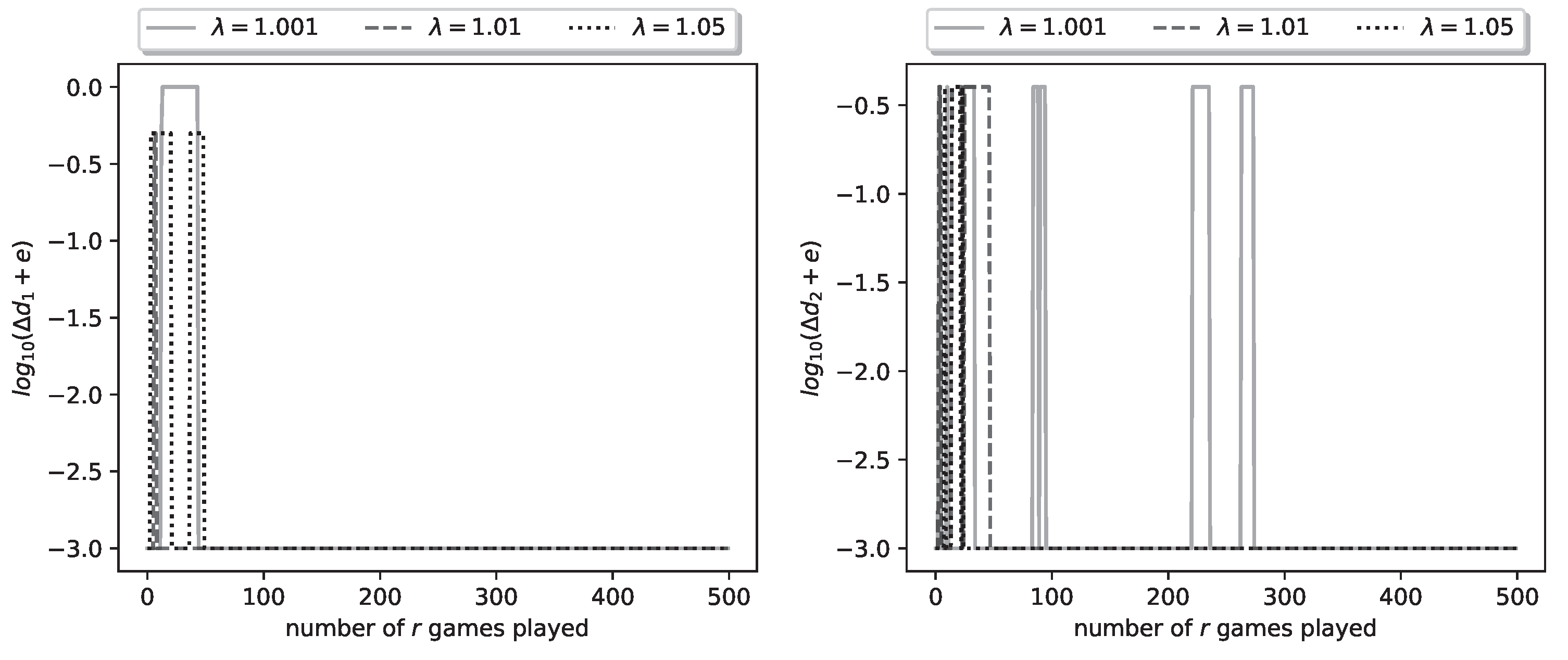
In Figure 9 we plot the logarithmic relative errors . These also, as expected, have converged to zero by the 300-th iteration.
Figure 9.
Plot of logarithmic relative errors , for a representative run of the learning process.
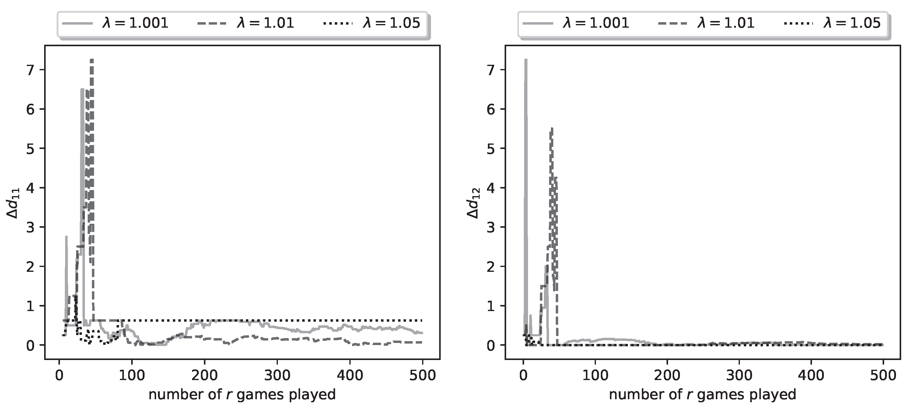
As in Group A, the fact that the estimates of the optimal shooting thresholds and strategies achieve zero error does not imply that the same is true for the kill probability parameter estimates. In Figure 10, we plot the relative errors and . The relative error converges to zero quickly, but the relative error does not converge to zero for . For the error converges to a fixed nonzero value, which indicates that the algorithm obtains wrong estimates. However, the error is sufficiently small to still result in zero-error estimates of the shooting thresholds.
Figure 10.
Plot of relative parameter errors , for a representative run of the learning process.
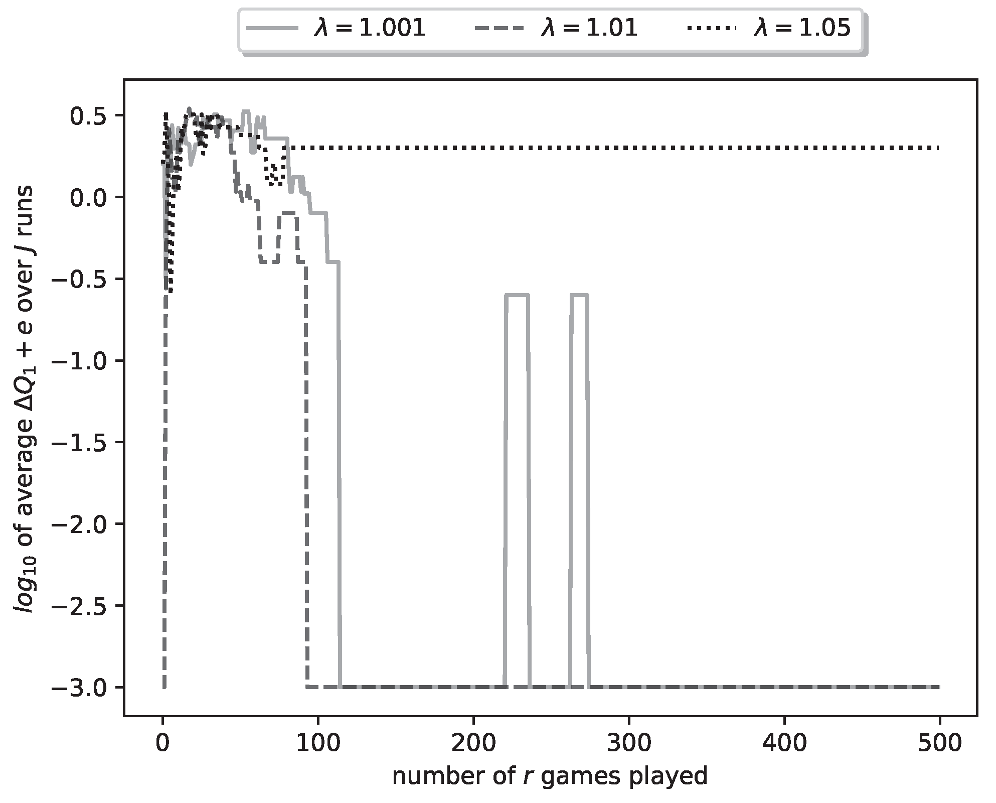
As in group A, to better evaluate the algorithm, we have run it for times and averaged the obtained results. In particular, in Figure 11 we plot the average of ten curves of the type plotted in Figure 4. Note that now we plot the curve for plays of the duel.
Figure 11.
Plot of (’s payoff) for a representative run of the learning process.
We again run the learning algorithm for various combinations of game parameters and record the average error attained at the end of the algorithm (again at ) for each combination. The results are summarized at the following tables.
From Table 6 and Table 7, we observe that for most parameter combinations, all learning sessions conclude with a zero for the smaller values. However, for , the algorithm fails to converge and exhibits a high relative error. Notably, increasing from 1.001 to 1.01 generally accelerates convergence, although this is not guaranteed in every case. In one instance, a higher (specifically ) leads to a slower average convergence of to zero, indicating the importance of initial random shooting choices. We also observe that results for the highest are suboptimal, with the algorithm failing to converge in varying numbers of sessions, such as in 1 out of 10 or even 5 out of 10 cases. Notably, when convergence does occur, it happens relatively quickly, with sessions typically completing in under 1000 iterations. These findings also highlight the trade-off between exploration and exploitation, as discussed earlier.
Finally, in Table 8 we see how many learning sessions were run and how many converged to zero error estimate for different values of D and .
5. Discussion
We proposed an algorithm for estimating the unknown game parameters and the optimal strategies through the course of repeated plays. We tested the algorithm for two models of the kill probability function and found that it converged for the majority of tests. Furthermore, we observed the established relationship between higher learning rates and reduced convergence quality, underscoring the trade-off between learning speed and stability in convergence. Future research could investigate additional models of the accuracy probability function, including scenarios where the two players employ distinct models, and work toward establishing theoretical bounds on the algorithm’s probabilistic convergence.
Author Contributions
All authors contributed equally to all parts of this work, namely conceptualization, methodology, software, validation, formal analysis, writing. All authors have read and agreed to the published version of the manuscript.
Funding
This research received no external funding.
Conflicts of Interest
The authors declare no conflicts of interest.
References
- Polak, Ben. Backward Induction: Reputation and Duels. Open Yale Courses. https://oyc.yale.edu/economics/ econ-159/lecture-16.
- Prisner, Erich. Game theory through examples. Vol. 46. American Mathematical Soc. (2014).
- Fox, Martin, and George S. Kimeldorf. “Noisy duels.” SIAM Journal on Applied Mathematics, vol.17, pp. 353-361 (1969).
- Garnaev, Andrey. “Games of Timing.” In Search Games and Other Applications of Game Theory. Berlin, Heidelberg: Springer Berlin Heidelberg, pp. 81-120 (2000).
- Radzik, T. “Games of timing related to distribution of resources.” Journal of optimization theory and applications, vol. 58, pp. 443-471 (1988).
- Roy, Dilip. “The discrete normal distribution.” Communications in Statistics-theory and Methods, vol. 32, pp. 1871-1883 (2003).
- Ishii, Shin, Wako Yoshida, and Junichiro Yoshimoto. “Control of exploitation–exploration meta-parameter in reinforcement learning.” Neural networks, vol. 15, pp. 665-687, (2002).
- Geman, Stuart, and Donald Geman. “Stochastic relaxation, Gibbs distributions, and the Bayesian restoration of images.” IEEE Trans. on pattern analysis and machine intelligence, vol. 6, pp. 721-741, (1984).
| 1 | This proposition is stated informally in [1]. |
| 2 | We use the same notation for several other quantities as will be seen in the sequel. |
| 3 | An analogous phenomenon occurs in connection to the “temperature parameter” T in simulated annealing [8] and many other learning algorithms. |
Figure 1.
Game tree example
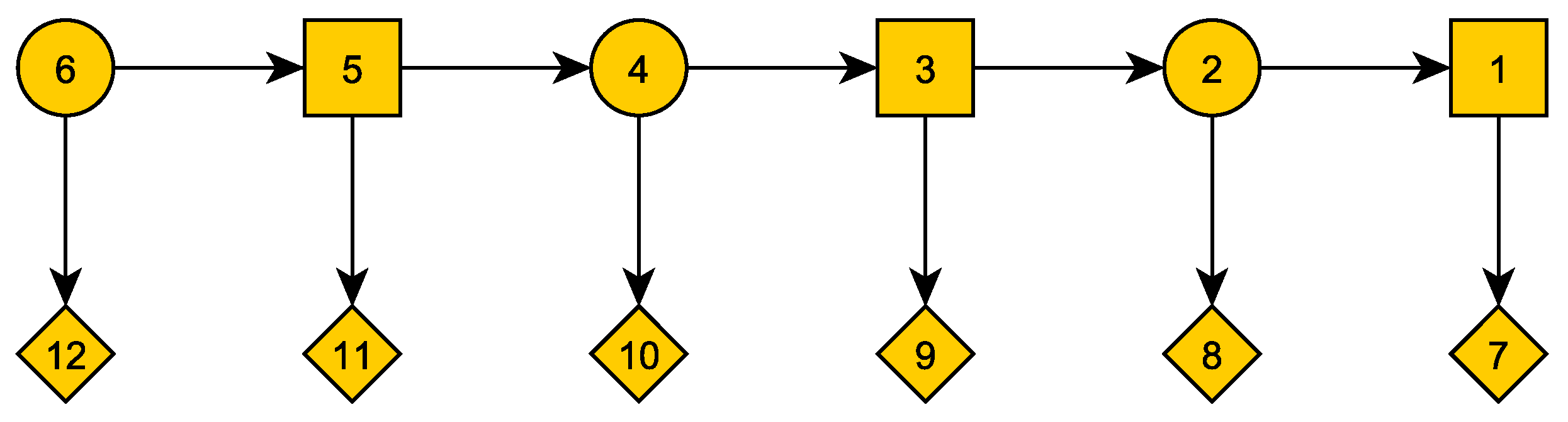
Figure 2.
Game tree example with values of terminal vertices.
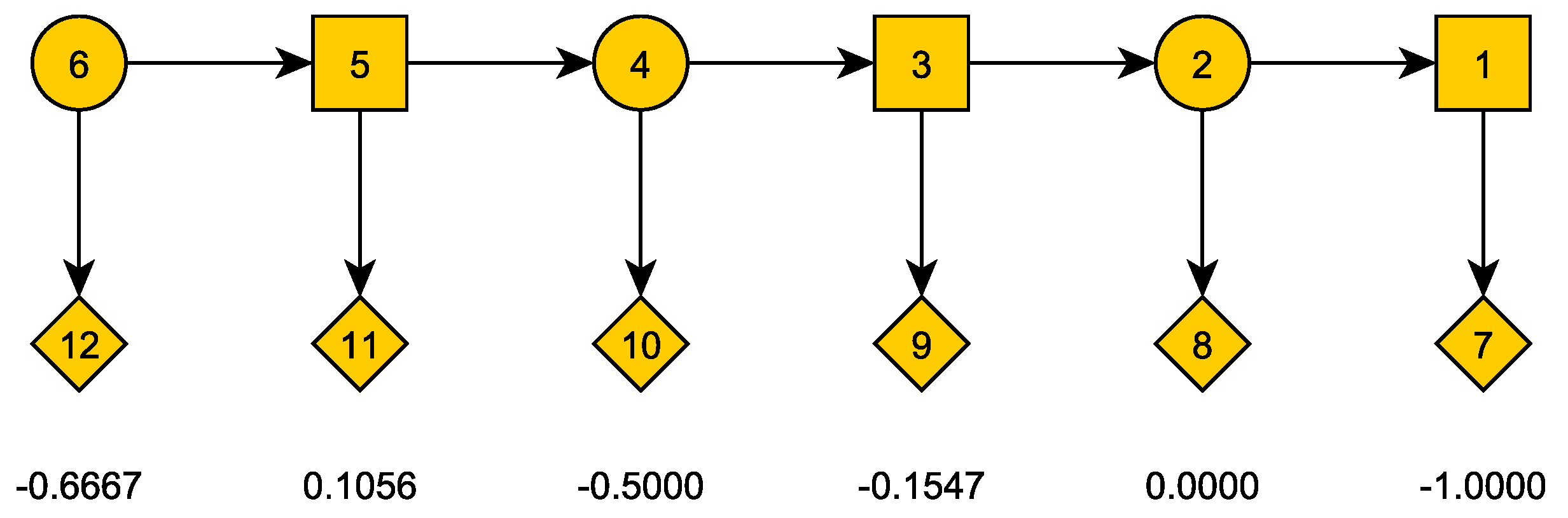
Figure 3.
Game tree example with values of all vertices
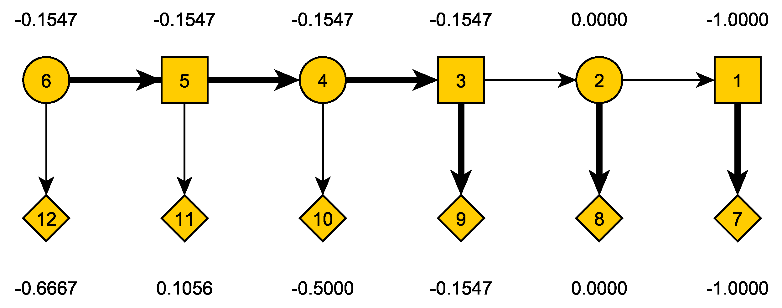
Table 1.
Kill probabilities
| d | 1 | 2 | 3 | 4 | 5 | 6 |
|---|---|---|---|---|---|---|
| 1.000 | 0.500 | 0.333 | 0.250 | 0.200 | 0.166 | |
| 1.000 | 0.707 | 0.577 | 0.500 | 0.447 | 0.408 |
Disclaimer/Publisher’s Note: The statements, opinions and data contained in all publications are solely those of the individual author(s) and contributor(s) and not of MDPI and/or the editor(s). MDPI and/or the editor(s) disclaim responsibility for any injury to people or property resulting from any ideas, methods, instructions or products referred to in the content. |
© 2024 by the authors. Licensee MDPI, Basel, Switzerland. This article is an open access article distributed under the terms and conditions of the Creative Commons Attribution (CC BY) license (http://creativecommons.org/licenses/by/4.0/).
Copyright: This open access article is published under a Creative Commons CC BY 4.0 license, which permit the free download, distribution, and reuse, provided that the author and preprint are cited in any reuse.


