Preprint
Article

This version is not peer-reviewed.

Unsupervised Modeling of E-Customers’ Profiles: Multiple Correspondence Analysis with Hierarchical Clustering of Principal Components and Machine Learning Classifiers

A peer-reviewed article of this preprint also exists.

Submitted:

04 November 2024

Posted:

06 November 2024

You are already at the latest version

Abstract

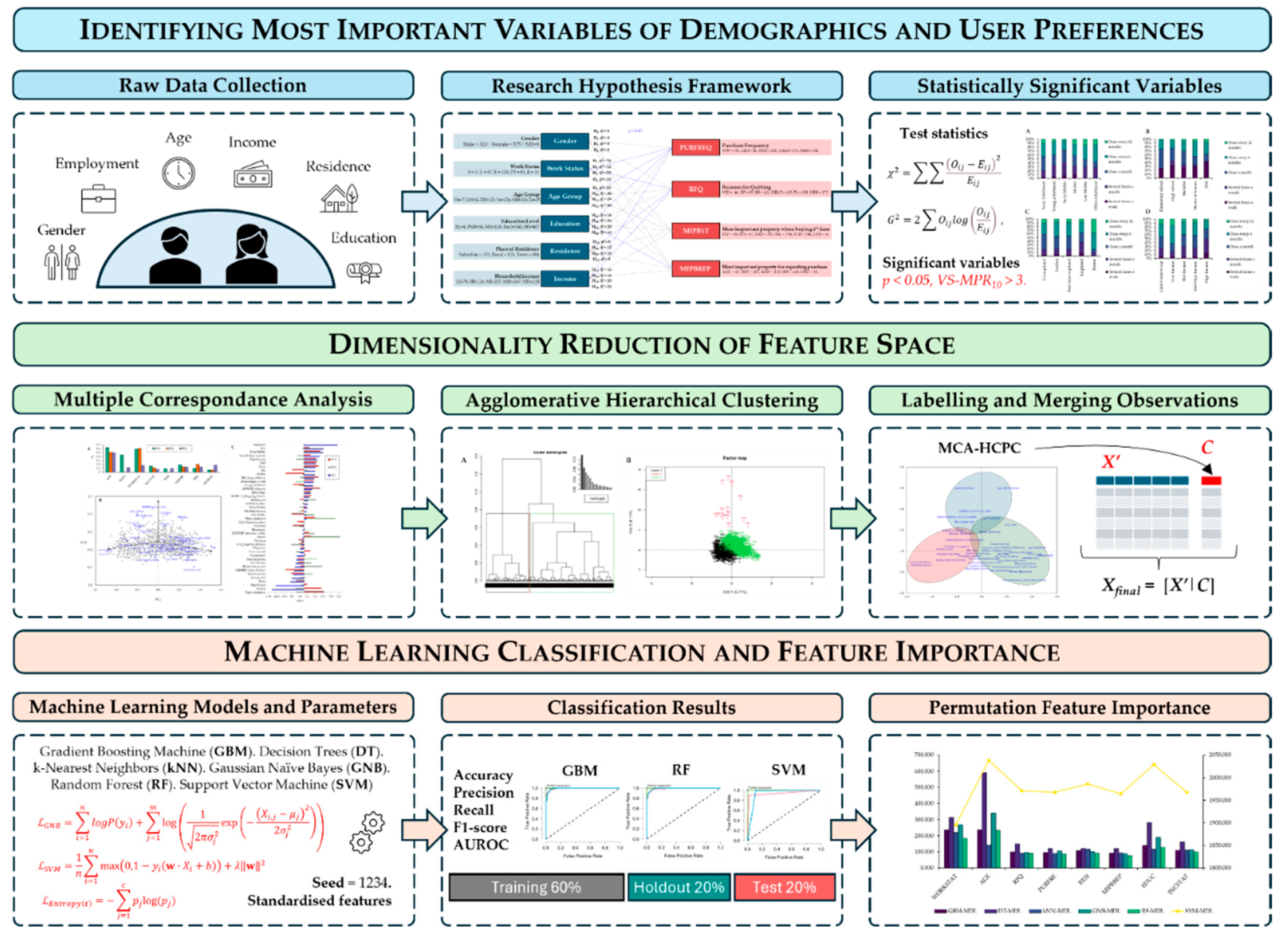
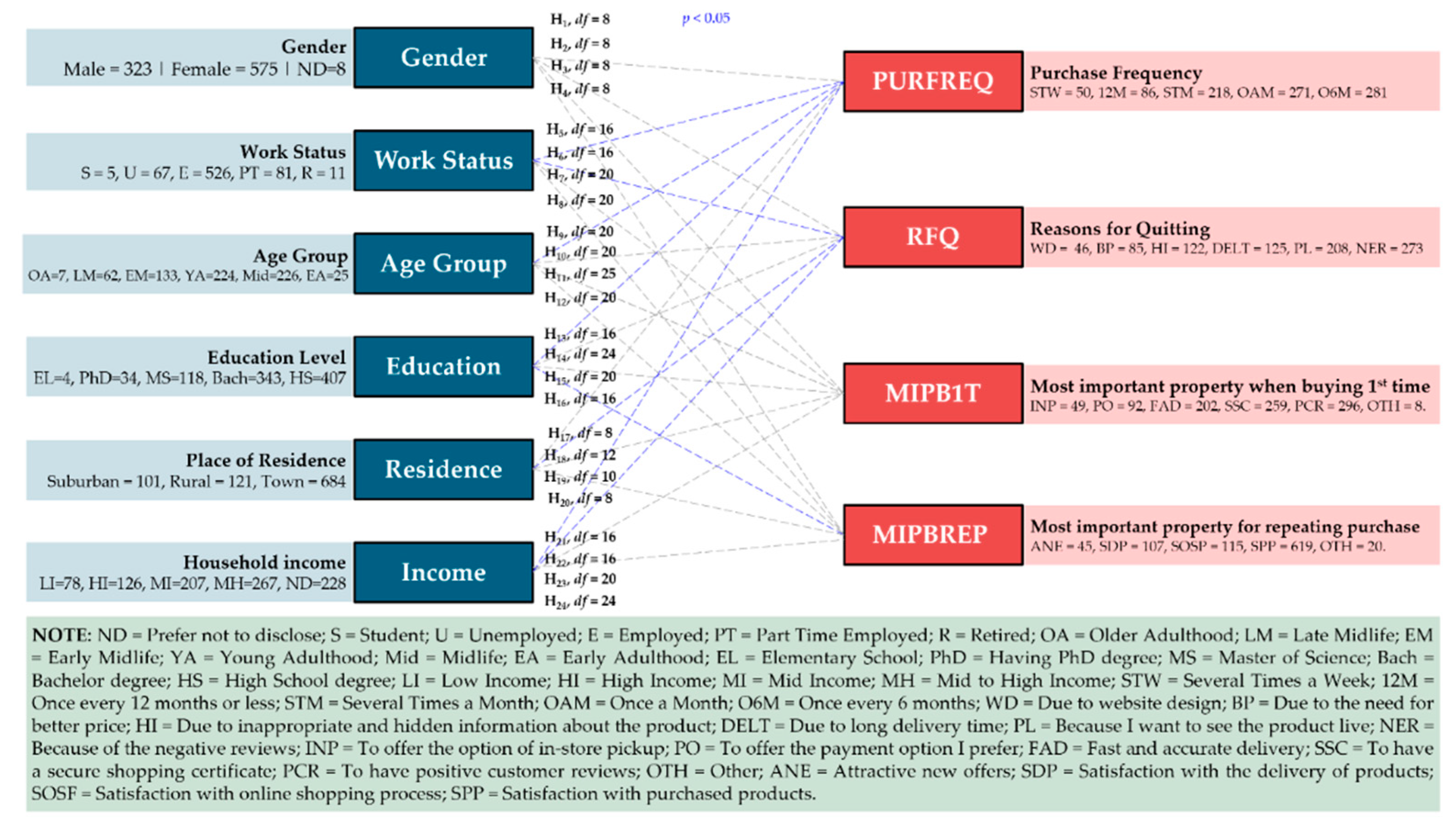
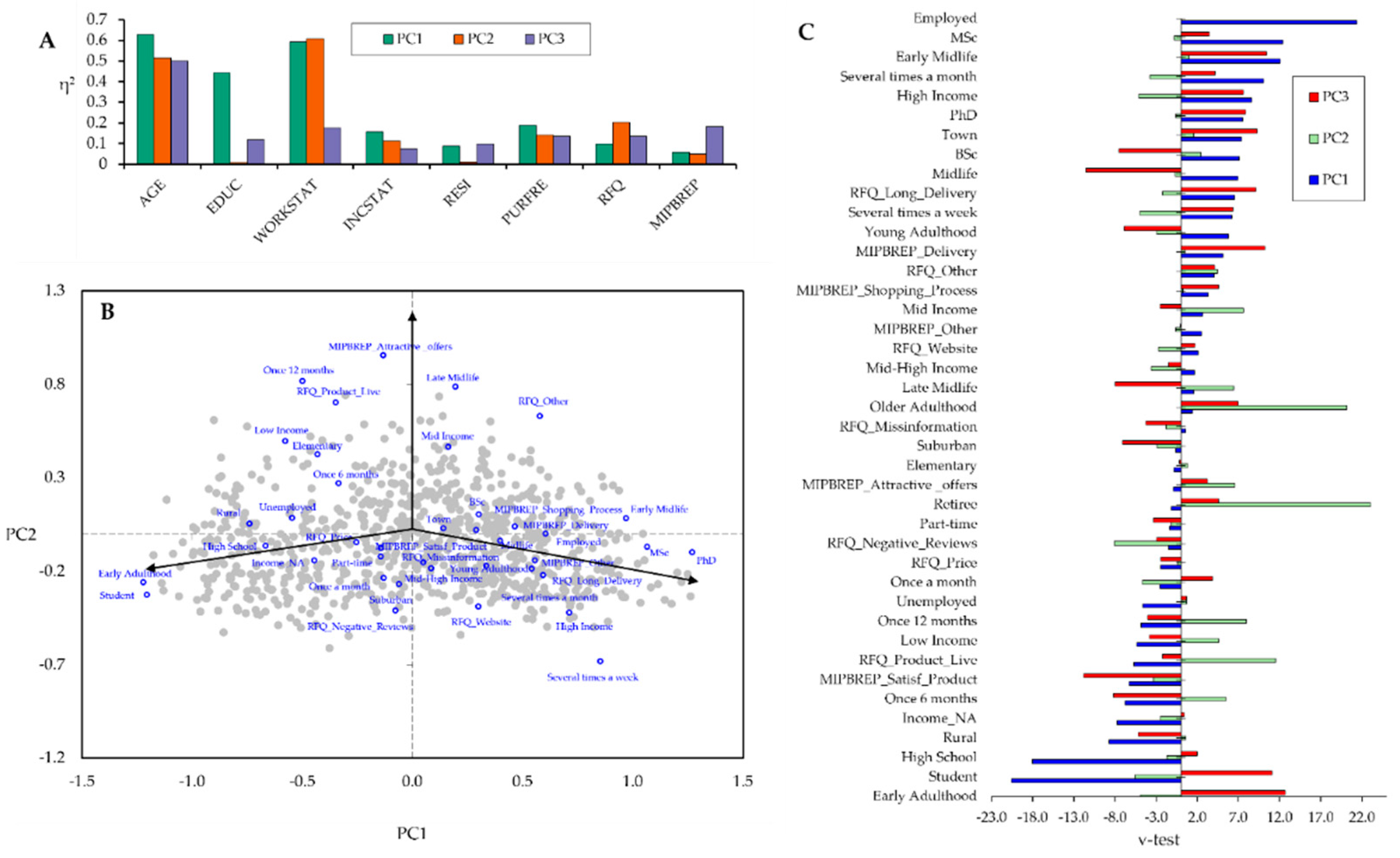
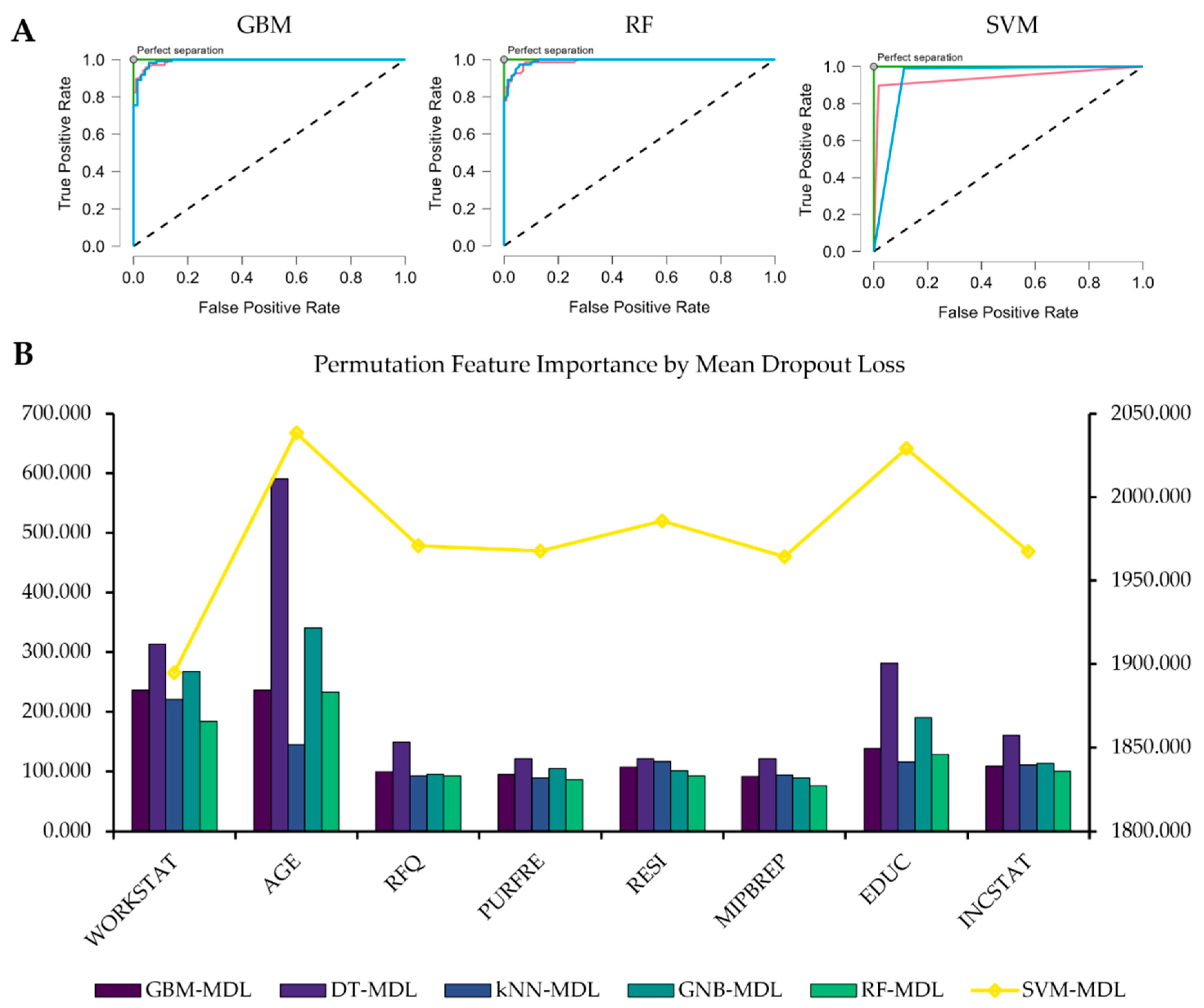
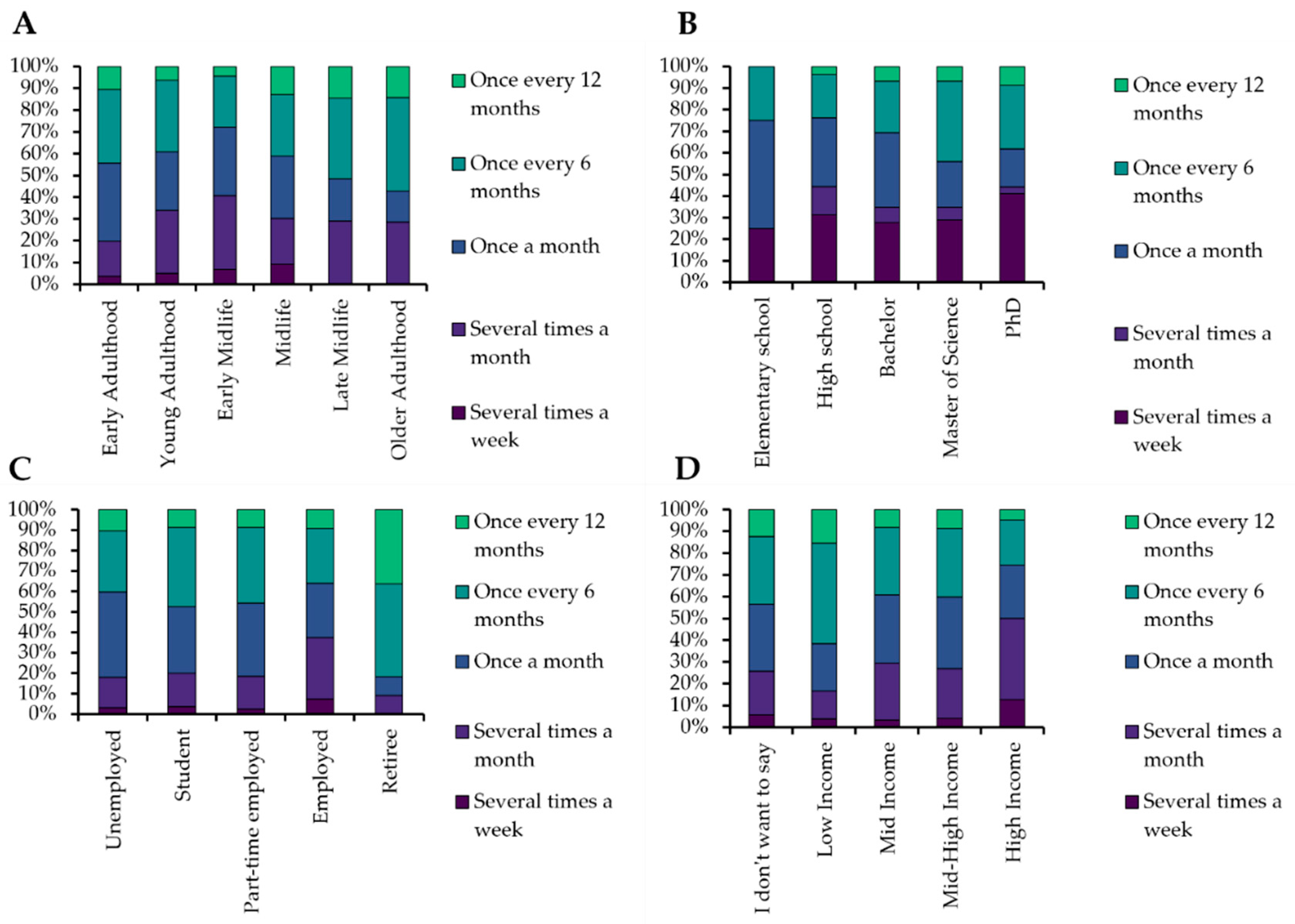
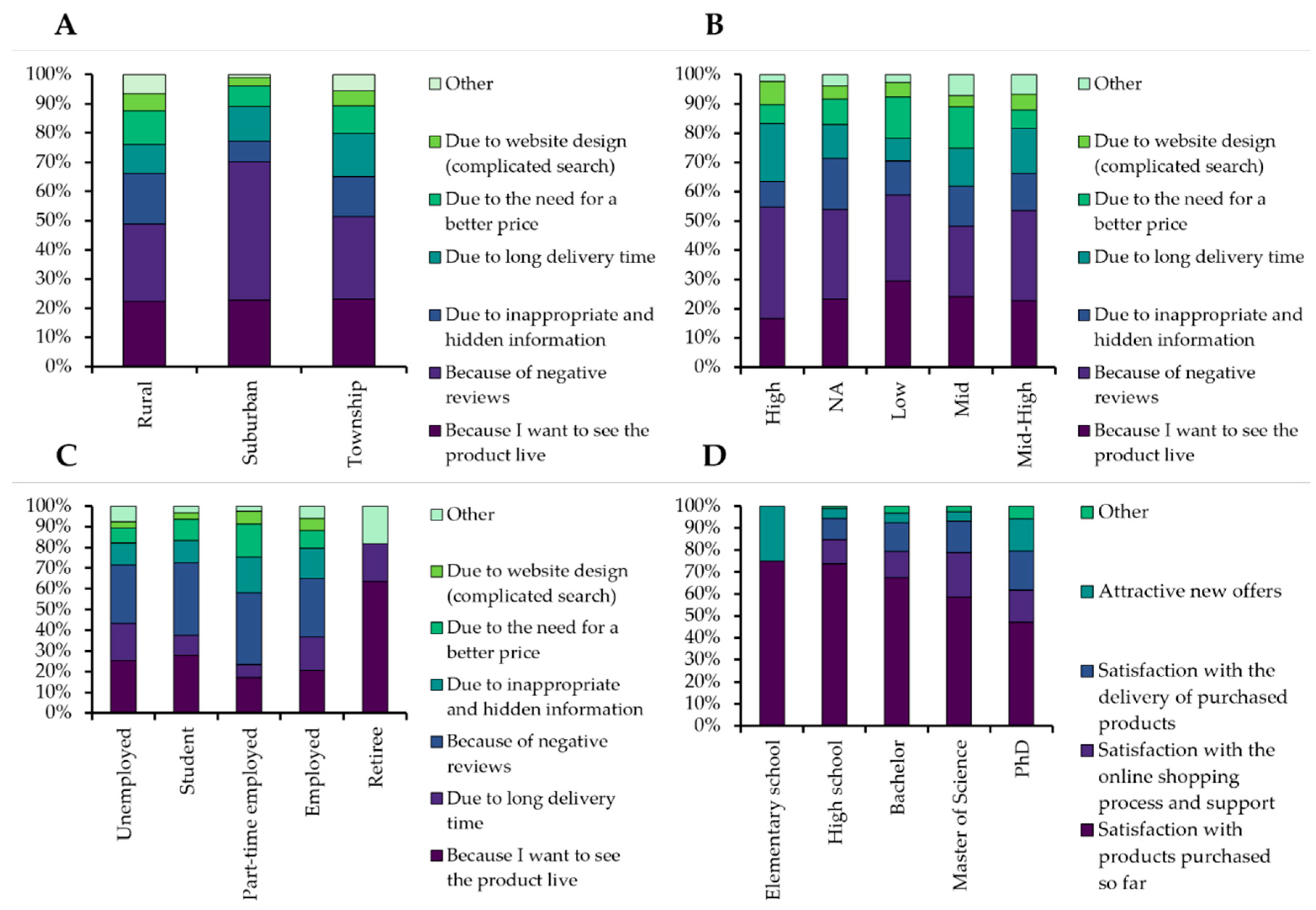
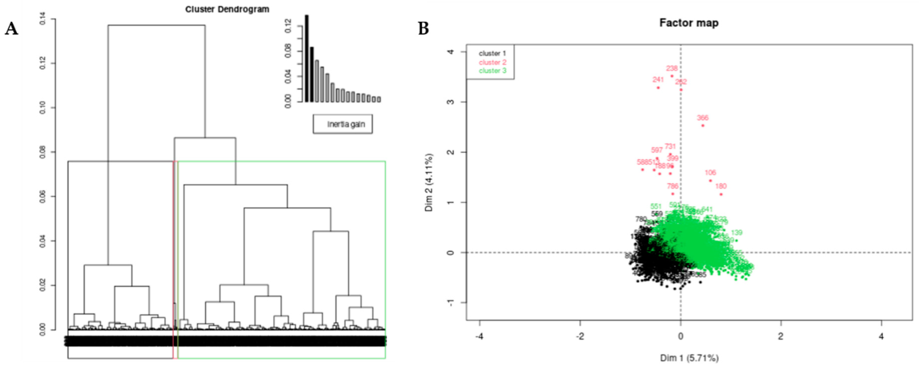
The rapid growth of e-commerce has transformed customer behaviours, demanding deeper insights into how demographic factors shape online user preferences. To understand the impact of these changes, this study performs a threefold analysis. Firstly, the study investigates how demographic factors (e.g., age, gender, education, income) influence e-customer preferences in Serbia. From a sample of n = 906 respondents, we test conditional dependencies between demographics and user preferences – “purchase frequency”, “the most important property when buying for the first time”, “the most important property before repeating a purchase”, and “reasons for quitting an online purchase”. From a hypothetical framework of 24 tested hypotheses, the study successfully rejects 8/24 (with p < 0.05), suggesting a high association between demographics with purchase frequency (p < 0.01) and reasons for quitting the purchase (p < 0.01). However, although reported test statistics suggest an association, understanding how interactions between categories shape e-customer profiles is lacking. As a consequence, the second part considers an MCA-HCPC (Multiple Correspondence Analysis with Hierarchical Clustering on Principal Components) to identify user profiles. The analysis reveals three main clusters : (1) young female unemployed e-customers driven mainly by customer reviews; (2) retirees and older adults with infrequent purchases, hesitant to buy without experiencing the product in person; (3) employed, highly educated, male midlife adults who prioritise fast and accurate delivery over price. In the third stage, the study uses identified clusters as labels for Machine Learning (ML) classification through the following algorithms: Gradient Boosting Machine (GBM), Decision Tree (DT), k-Nearest Neighbors (kNN), Gaussian Naïve Bayes (GNB), Random Forest (RF) and Support Vector Machine (SVM). The results suggest high classification performance of GBM (AUROC = 0.994), RF (AUROC = 0.994) and SVM (AUROC = 0.902) in identifying user profiles. Lastly, after performing Permutation Feature Importance (PFI), the findings suggest that age, work status, education, and income are the main determinants of shaping e-customer profiles and developing marketing strategies.

Keywords: 
;  ;  ;  ;  ;  ;  

1. Introduction

1.1. Background and Rationale

E-commerce is developing faster than ever, with an increase in the number of transactions [1,2]. This global trend allows retailers to expand their reach with as many customers as possible [3]. Additionally, the COVID-19 pandemic has further accelerated the change in consumer habits, with many consumers switching to online shopping [4,5] posing new challenges to e-tailers [6,7,8]. With the rise of online consumers, e-tailers are forced to improve customer experience throughout the purchasing process [9,10]. Similar trends are visible in the Serbian market, where e-shopping is becoming pronounced, emphasising the importance of e-commerce in modern business.
According to Ranđelović [11], despite the numerous benefits of e-commerce, consumers in Serbia still need to accept this form of commerce. One of the reasons for the slow adoption of e-commerce is consumer distrust, especially regarding the security of transactions [12]. Still, in 2023, the e-commerce market in Serbia grew by 34.5%, reaching a value of 955.7 million dollars, while it is predicted that by 2027, the market will grow to 1.65 billion dollars. The growth in e-commerce users is estimated to reach 4.36 million customers by 2027, making up 62.5% of Internet users in Serbia [13]. Regardless of these positive trends, Serbia faces challenges such as the preference for cash on delivery payments and the continued lack of trust in the security of online transactions [14].
Demographic data, such as gender, age, income and education, are vital in analysing consumer preferences and behaviour [15,16]. These variables enable market segmentation and adaptation of marketing strategies to the specific needs of different consumers [17]. For example, income often indicates purchasing power and can help target marketing campaigns to different socio-economic segments [18]. Education and age influence how consumers use technology and how they behave when shopping online [19]. Understanding these demographic factors allows e-tailers to identify target groups and optimise customer experience [20]. In Serbia, where e-commerce is growing, insight into demographic variables can help overcome obstacles and improve consumer acceptance of e-commerce. This provides valuable information for adjusting e-tailers' market strategies and improving user experience.

1.2. Literature Review

When analysing user profiles in e-commerce and the influence of demographics, limited studies include supervised or unsupervised learning models. Previous studies primarily rely on user descriptive profiles and inferential statistics for hypothesis testing [1,16,21,22], while others extend the analysis with multivariate regression [23] and factor models [24,25,26] whereas item answers are used as continuous values assuming a normal distribution. In addition, we have identified a sample of studies that use advanced mathematical modelling of e-customer profiles. For example, Hristoski, I. et al. [27] Using customer behaviour model graphs (CBMGs), identify 12 typologies of online shoppers. The CBMGs work as an N×N transitional probability matrix that denotes relative frequencies of invoking specific e-commerce functions. These frequencies are then used to map a unique transitional probability matrix of users with similar behaviour. Next, Swarnakar, P. et al. [28] use Logistic Regression (LR) and Artificial Neural Networks (ANN) to predict online purchase behaviours to help e-retailers develop suitable strategies. They first perform a statistical analysis of demographics and user preferences to identify relevant factors affecting online behaviour before using LR and ANN to predict user behaviour. In a vice versa approach, Chen, X. et al. [29] used deep learning algorithms to predict user demographics based on the multisource user characteristics and preferences data.
On the other hand, some have tried identifying user profiles through cluster modelling. For instance, Bellini, P. et al. [30] perform k-means clustering to identify user profiles based on demographics and preferences. The results show that after identifying different clusters of user profiles, a stimulus was generated for the customers, which increased buyers' purchases by 3.48%. The Kuruba, Y. et al. [31] Customer segmentation was successfully performed by relying on distributed clustering models. Lastly, a study by Hørlück, J. et al. [32] The study fails to identify clusters of user behaviour using an unsupervised Gaussian Mixture Model with Hierarchical Probabilistic Clustering. It neither falsifies nor supports the hypothesis of identifying clear user profiles based on buying behaviour.
Furthermore, understanding that demographics play an important role in shaping user profiles, we provide a brief overview of demographic variables affecting user preferences. The literature reports that e-customers between the ages of 18 and 50 are the most active [33] with young adults being prevalent [34,35], mainly driven by convenience and interactivity [36]. Older adults tend to value product selection and post-consumption for repurchases [37], while younger adult. The studies on gender suggest an inconclusive contribution [38,39,40], reporting both significant and non-significant findings. However, some suggest that women are “shopping for fun” while males emphasise “quick shopping” behaviours [41]. Additionally, Naseri & Elliott [42] suggests that education significantly influences the adoption of online shopping [43,44,45,46], while also income status [47,48] plays an important role, where both income and education tend to have a higher probability of online shopping [49,50]. Lastly, we have identified that employment (work status) also determines purchase behaviours [51,52,53]. A more comprehensive list of demographics that may be of interest to the reader is described elsewhere [54,55].
The major challenges still exist. Although proposed typologies, clusters or classes of user profiles can be successfully mapped into different user profiles, the biggest issue is that most clusters and user profiles overlap and are not mutually exclusive. Also, from previous studies, there is a lack of evidence and methods describing the actual contribution of each individual variable (features) in describing contribution or shared variance. In this study, we first delve into unsupervised modelling of user profiles for obtaining cluster labels; after this, we use Machine Learning (ML) classification algorithms to predict user-profiles and identify the most important features.

1.3. Aims and Objectives

Considering the research problem's contextual settings, the study's primary idea is to switch from a traditional statistical exploratory analysis to an ML approach in identifying user profiles of e-customers. Firstly, we examine how demographic factors influence the online behaviour of e-customers in Serbia. Specifically, we are interested in how the demographics above affect four selected user behaviour factors: Purchase frequency (PURFREQ), Most important property when buying the first time (MIPB1T), Most important property before repeating the purchase (MIPBREP), and Reasons for quitting the online purchase (RFQ) using a hypothetical framework.
However, given that statistical testing highlights significant relationships between categories, it needs to provide an understanding of how these categories interact. As a response, we perform multiple correspondence analysis with hierarchical clustering on principal components (MCA-HCPC) as an unsupervised model for labelling user profiles. Secondly, after obtaining class categories, i.e., labels, we perform ML classification using a dataset from user profiles that includes demographics and user preferences. Lastly, we use the best-performing algorithms to allocate the most important features using Mean Dropout Loss (MDL) from the obtained classification results.
The rest of the study is structured as follows. The second section provides an in-depth description of the survey used for the study. In addition, we provide rigorous data analysis procedures, starting from a priori sample determination, study selection and proposition of hypotheses in the study. The third section provides information about descriptives, including demographics and user behaviour variables. Next, we provide significant and non-significant results to ensure the transparency and replicability of the findings. Also, given that existing association tests fail to provide exact interaction between categories, we perform MCA to provide a deeper understanding of the association between variables, including all variables in the study and reduction of variables to only those reported as statistically significant. The study provides a discussion section that informs about the findings obtained, and finally, it provides concluding remarks, limitations, and implications of the study in the last section.

2. Materials and Methods

2.1. Multistage Model of Data Workflow Framework

Data workflow framework consists of three stages (Figure 1). The first stage explains a priori sample sample determination, survey development and data collection. Also, this stage explains research hypothesis framework for the reduction of a raw dataset to a dataset comprising only of statistically significant association. Lastly, the first stage explains an in-depth statistical analysis regarding the statistically significant association between demographics and user preferences.
The second stage explains Multiple Correspondence Analysis (MCA) procedure for reducing dimensionality of a dataset into two dimensional space. Next, the study extracts relevant features by including only top two principal components that explain the most variation, i.e., inerta. Also, the Agglomerative Hierarchical Clustering (AHC) is performed on MCA’s principal components for obtaining clusters of user preferences. Following the procedure of identifying class labels, i.e., user profiles, we merge the class label vector with raw dataset.
The third segment proposes and explains utilised ML classifiers, i.e., ML algorithms, setting the parameters and loss functions used for the analysis. The second part of the third stage describes main classification metrics used for evaluating the model performance and ML classification performance metrics – Accuracy, Precision, Recall, F1-score and AUROC. Finally, the last part of the stage includes extraction of the most relevant features using Permutation Feature Importance (PFI) [56] that builds upon Mean Dropout Loss (MDL) metric [57].

2.2. Data Collection and Sample Size

The research was realised during the four weeks of November-December 2022 using two strategies for securing a representative sample. The survey was created on the Google Forms platform and distributed exclusively online. The target group was adult citizens of the Republic of Serbia who had experience ordering goods and durable products via the Internet and delivering them to a specific location. The survey included respondents with experience delivering goods such as electrical appliances, clothing, footwear, furniture, tools, small home and yard use items, sports equipment, and similar items. Before participating in the survey, respondents gave their consent to participate. They were informed about the research objectives and that their answers would be anonymous and analysed in groups. They were informed that they could stop participating at any time.
A priori sample size was determined as follows. Firstly, we conduct sample size estimation to estimate the minimum required sample size for performing χ2 test statistics. To do so, we used G*Power (v.3.1.9.6) for calculating sample size per parameters: Effect size w = 0.3 (medium effect), α = 0.05, Power (1-β error probability) = 0.80 and df = 36 (determined as the most of 7 categories per variables j and k, such that df = (j-1)(k-1)). The output statistic shows non-centrality parameter λ = 26.46, with χ2crit = 50.998, actual Power (1-β error probability) = 0.801, and minimum sample size of n = 294. Secondly, we rely on sample size calculation per Hamburg [58] – a commonly used sample size calculator can be found online (e.g., https://www.calculator.net/). The minimum required representative sample is n = 385. Lastly, given the sample size from previous similar studies [41,46] was higher than required, we have also stopped data collection at n = 906 respondents.

2.3. Research Hypothesis Framework

The research hypothesis framework (Figure 2) is designed to test the conditional dependencies, i.e., the existence of an association between different demographic properties of e-consumers and user preferences (and behaviour). To do so, we included variables primarily reported in previous studies [33,59] regarding demographic properties, e.g., gender, work status, age group, education, place of residence, and income. Next, we test the association with PURFREQ (Purchase frequency), MIPB1T (Most important property when buying the first time), MIPBREP (Most important property before repeating the purchase), and RFQ (Reasons for quitting the online purchase).
For hypothesis testing, Pearson’s χ2 test statistic is chosen, described as follows:
χ 2 = O i j E i j 2 E i j   ,
such that Oij is observed frequencies, Eij is expected frequencies computed as Ri × Cj/N, where Ri and Cj represent row and column marginals, while N is the total observations. However, we also included G2 likelihood ratio:
G 2 = 2 O i j l o g O i j E i j   ,
as a more robust method for evaluating the goodness-of-fit and association between variables in contingency tables. Given that the χ2 statistic is only approximated by the χ2 distribution and worsens when expected frequencies are relatively small, which is a common controversy using χ2 test statistic, we consider including G2 because it provides more robust measurements for large dimensional tables. It is commonly discussed that G2 advantage over traditional χ2 is that G2 for large contingency tables can be neatly decomposed into smaller components [60], which cannot be done by χ2 test. Even so, as the sample size increases, statistics tend to converge. The degrees of freedom df is determined by df = (r-1)(c-1), where r and c represent classes of row and column profiles, respectively.
Furthermore, we analysed the diagnosticity of p values using the VS-MPR (Vovk-Sellke Maximum p-Ratio) calibration score. The score is computed as VS-MPR = -e × p × ln(p) and is commonly referred to as a lower bound to BF (favouring H0 over H1)[61]. The reason for including VS-MPR is that a large body of research [62,63,64] is calling into question the traditional threshold (p < 0.05) for deciding whether a model is statistically significant, i.e., rejects the null hypothesis. We consider the following labelling intervals as evidence in favour of the alternative over the null hypothesis: VS-MPR10 = 1-3 anecdotal, VS-MPR10 = 3-10 substantial, VS-MPR10 = 10-30 strong, VS-MPR10 = 30-100 very strong, and finally VS-MPR10 > 100 as decisive evidence [65].

2.4. Multiple Correspondence Analysis Hierarchical Clustering of Principal Components

To understand MCA's description, let the initial raw dataset be a matrix X ∈ ℝn×m, where n is the number of observations and m is the number of variables that explain demographics and user preferences. To reduce the dimensionality of dataset X, we first perform hypothesis testing (see eq.2 and eq.3) to keep only statistically significant variables (p < 0.05, VS-MPR10 > 3). After the removal of non-significant variables, the reduced X’ ⊂ X dataset comprises only significant variables. Hence, the X is then subjected to MCA to further reduce dimensionality by transforming raw categorical data into Principal Components (PCs).
The first step in MCA is to convert a raw categorical dataset X into indicator matrix Z ∈ ℝn×q, where q is the number of class categories from the retained variable set. Next, from the defined indicator matrix Z, we perform centring by subtracting row, and column means to obtain centred matrix ZC:
Z C ,   i j = Z i j 1 n i = 1 n Z i j 1 q i = 1 n Z i j + 1 n q i = 1 n j = 1 q Z i j ,
which adjusts for marginal distributions ensuring standardised matrix for PC extraction. Using Singular Value Decomposition (SVD) we decompose ZC as follows:
Z C = U Σ V T   ,
where U ∈ ℝn×k are singular vectors in the reduced space, Σ ∈ ℝk×k is a diagonal matrix with singular values of each PC, and V ∈ ℝq×k is the singular vector matrix representing variable contributions of each individual PC. The selection of top k components is performed based on the first two PCs that explain the most variance as PCs ∈ ℝn×k.
Finally, after obtaining reduced dataset PCs, an HCPC is performed for identifying clusters, i.e., labeling user profiles in a reduced space. For performing distance computation and obtaining distance matrix D, an Euclidian distance D(i,j) between each pair of observations in PCs are performed:
D i , j = P C s i P C s j   2 ,
which yields distance matrix D ∈ ℝn×n capturing similarities between respondents. For applying hierarchical agglomerative clustering on PCs, Ward’s method is selected for merging clusters and minimising within-cluster variance. The results are represented via dendrogram. Selection of clusters C is performed by linkage L assiging labels to observations C = {c1, c2, …,cn}. As a last step, we merge cluster C labels with dataset X’ resulting in final dataset Xfinal = [X’|C], which is then subjected to classification by ML algorithms.

2.5. Machine Learning Classifiers

Machine learning classification is performed as follows. Let dataset Xfinal ∈ ℝn×(m+1) be the final dataset, where n is the number of observations and m represents the features (demographics and user preferences), while the last column, denoted as y ∈ {1, 2, …, c}, represents the cluster labels assigned via MCA-HCPC, such that c represents total number of selected clusters.
We first perform splitting the dataset into train/test dataset, such that Xtrain ∈ ℝntrain×m be training matrix with ytrain ∈ {1, 2, …, c}ntrain labels. Similarly, let Xtest ∈ ℝntest×m be training matrix with ytest ∈ {1, 2, …, c}ntest be the test dataset. Our goal is to train the ML classifier : Xtrain y by optimising loss function . For proposed ML classifiers – Gradient Boosting Machine (GBM), Decision Tree (DT), k-Nearest Neighbors (kNN), Gaussian Naïve Bayes (GNB), Random Forest (RF), and Support Vector Machine (SVM) – the loss functions are defined for GBM:
L G B M = i = 1 n j = 1 c y i , j l o g ( y ^ i , j ) ,
where in multiclass problem yi,j is a binary indicator (1 if label j, otherwise 0), and y ^ i,j is the predicted probability for class j. For DT and RF a Gini impurity is estimated as:
L G i n i t = 1 j = 1 c p j 2 ,
and Entropy as:
L E n t r o p y t = j = 1 c p j l o g ( p j ) ,
where algorithms select the feature that maximises the reduction in Gini (or Entropy). For Gaussian Naïve Bayes, the classifier calculates posterior probability for each class:
L G N B = i = 1 n l o g P y i + j = 1 m l o g 1 2 π σ j 2 e x p X i , j μ j 2 2 σ j 2 ,
where P(yi) is the prior probability of class yi, while µ is the mean and σ2 is the variance of feature j conditioned on yi. The SVM loss function is determined per Hinge loss:
L S V M = 1 n i = 1 n max 0,1 y i w X i + b + λ w 2 ,
where yi ∈ {-1, 1} represents the true class label, w is the weight vector, whilee Xi is the feature vector, b is the bias, and λ is the regularisation parameter controlling the margin. Given that we face classification problem, the selection of highest performing algorithm is conducted per classification evaluation metrics of Accuracy:
A c c u r a c y = T P + T N T P + T N + F P + F N ,
where TP = True Positive, TN = True Negative, FP = False Positive, FN = False Negative. The Recall is calculated as:
R e c a l l = T P T P + F N   .
The Precision is estimated as:
P r e c i s i o n = T P T P + F P   ,
and finally F1-score is calculated as:
F 1 s c o r e = 2   T P 2   T P + F P + F N   ,
for estimating the classification performance of ML algorithms. Additionally, given that we encounter a multi-class classification problem, we also provide Receiver Operating Characteristic (ROC) curve, and estimate Area Under ROC (AUROC) by adopting it to multi-class problem.
For assuring transparency and replicability of the results, the following parameters are set for the ML models. For GBM we set the Shrinkage = 0.1, with 1.0 interaction depth with minimum number of observations per node = 10. The training used per tree is 50%. The number of trees is optimised such that maximum number of trees is 100. For DT algorithm, the minimum number of observations for split is 20 with minimum number of observations in terminal = 7, with maximum interaction depth = 30. The DT tree complexity is optimised with maximum complexity penalty = 1.0. The kNN algorithm settings are set: weights = Rectungular with Euclidian distance metric used. The number of nearest neighbors is optimised such that maximum allowed nearest neighbors = 10. For RF algorithm the training data used per tree is 50%, while features are split automatically with optimised number of trees set to maximum of 100 trees. The SVM algorithm is set with the following parameters: Weights = Linear, Tolerance of termination criterion = 0.001, with function ξ = 0.01. The costs of constraints violation is optimised with maximum violation cost = 5. Lastly, there were no smoothing parameter set for GNB algorithms, however, all algorithms contain scaled features and seed is set 1234.

3. Results

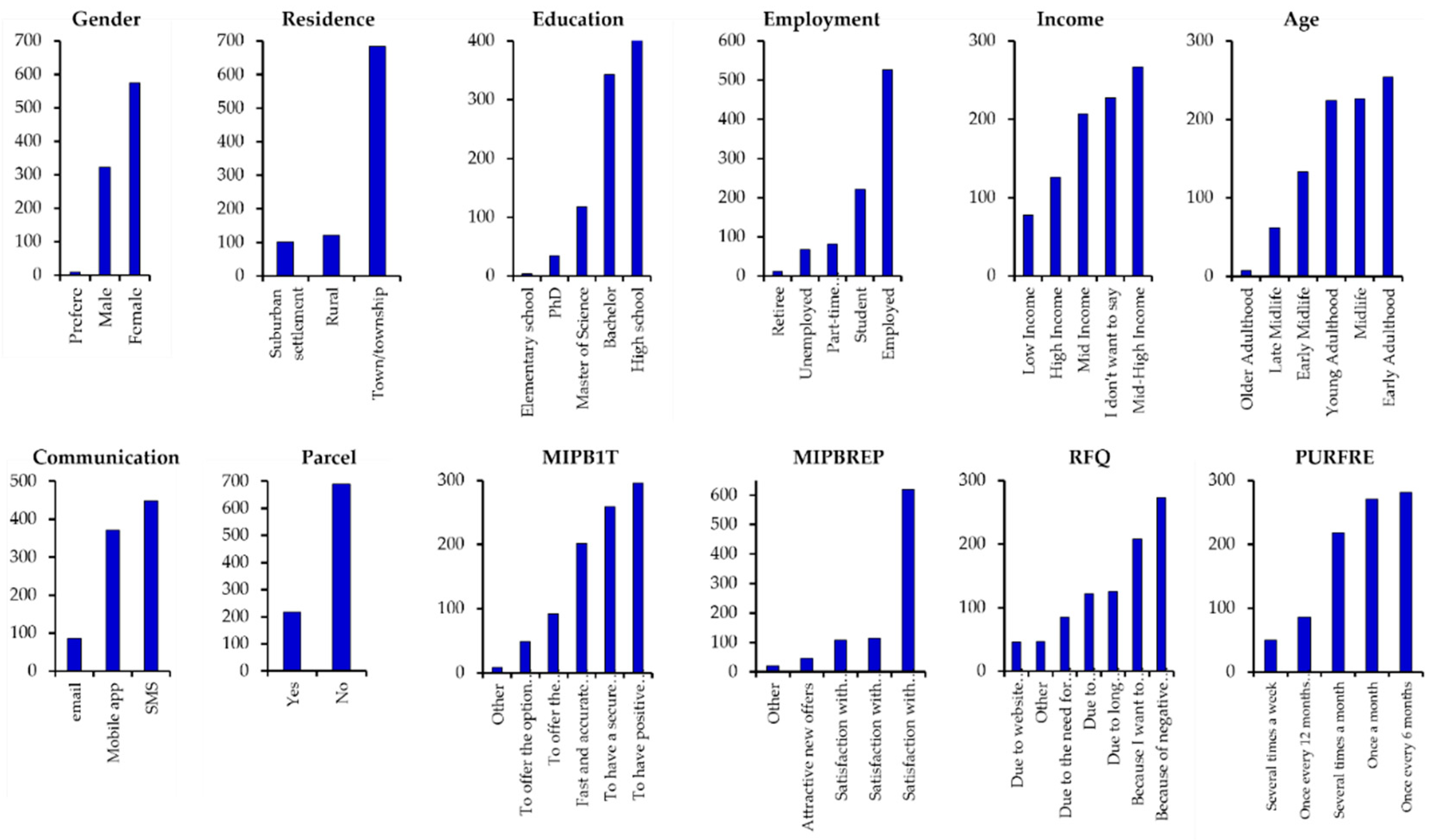
3.1. Descriptive Statistics

The characteristics (Figure 3) show the following. The study comprises 906 participants, ranging from 21 to 77 years old (Median = 34.90, SD = 12.67). Most were female (63%, n = 575), while <1% of participants selected “preferred not to disclose” (n = 8). Most of the respondents had completed high school (44.92%, n = 407), followed by a Bachelor’s degree (37.86%, n = 343) and a Master’s degree (13.02%, n = 118). The respondents were primarily situated in towns (75.5%, n = 684), followed by rural (13.36%, n = 121) and suburban areas (11.15%, n = 101). The employment characteristics show that 58% (n = 526) of respondents are employed. The income status is classified according to monthly earnings of RSD (Republic Serbia Dinar) in categories as Low Income (<50.000 RSD), Mid Income (50.000-100.000 RSD), Mid-High Income (100.000 – 200.000 RSD), High Income (>200.000 RSD). The results show that most respondents had Mid-High Income (29.47%, n = 267), 25.17% (n = 228) did not want to say their income, followed by Mid Income (22.85%, n = 207), High Income (13.91%, n = 126), and Low Income (8.61%, n = 78). Lastly, the age distribution shows average AVGAge = 35.914 with SDAge = 12.671, ranging from 21 to 77 years old. The age distribution is then coded as follows: Early Adulthood (18-24 years), Young Adulthood (25-34 years), Early Midlife (35-44 years), Midlife (45-54 years), Late Midlife (55-64 years), Older Adulthood (>65 years). As per coded categories, the descriptives show that Early Adulthood (28.04%, n = 254) is the most dominant category, followed by Midlife (24.94%, n = 226) and Young Adulthood (24.72%, n = 224), Early Midlife (14.68%, n = 133), Late Midlife (6.84%, n = 62), Older Adulthood (0.77%, n = 7).
Supplementary items such as “What communication channel would you prefer to have with the supplier?” labelled as Communication, and “Used parcel locker?“ show that most users prefer SMS (49.56%, n = 449) and Mobile App (40.95%, n = 371) and uses parcel locker (24.06%, n = 218), respectively. The main preferences, such as MIPB1T, show that most users consider positive reviews (32.67%, n = 296) when buying the first time, followed by “To have a secure shopping certificate” (28.59%, n = 259), and “Fast and secure delivery” (22.30%, n = 202). The MIPBREP property suggests that “Satisfaction with products purchased” (68.32%, n = 619) is the most dominant reason for repeating the purchase, followed by “Satisfaction with the online shopping (12.69%, n = 115), “Satisfaction with the delivery of purchased products” (11.81%, n = 107), and others. The RFQ shows that negative reviews (30.13%, n = 273), followed by “Because I want to see the product live” (22.96%, n = 208) and “Long delivery time” (13.80%, n = 125) are the most common reasons why users quiet their purchase. Lastly, the PURFRE show that most users buy every six months (31.02%, n = 281), followed by “Once a month” (29.91%, n = 271).
We construct contingency tables before performing the statistical inferential statistics and χ2 tests to investigate the association between variables. However, due to the limited length and extensive number of tables (24 tables) for each model comparison, the complete analysis with tables is provided in supplementary material in cases the reader is interested in following the complete analysis. In the following, we provide the final results of each model comparison using both χ2 and G2 test statistics, including the effect size (for χ2 test) and VS-MPR ratio.

3.2. Hypothesis Testing

After performing hypotheses testing as a proposed framework, we have rejected 8/24 hypotheses regarding the conditional dependencies, i.e., the association between e-customer demographics and user preferences (Table 1). Namely, we have only considered cases where both χ2 and G2 suggest statistically significant association (p < 0.05) and where there is at least moderate, i.e., substantial evidence in favour of the alternative hypothesis (VS-MPR10 > 3). In such instances, we consider that results will be more robust and reliable than previous findings. We additionally provided all other non-significant test results in the appendices (Table A1).
Surprisingly, no evidence suggested that demographic properties are conditionally dependent, i.e., associated with MIPB1T (p > 0.05). There is, however, anecdotal evidence (VS-MPR10 = 2.386) suggesting that Age (χ2 = 37.455, p = 0.052) tends to be associated with MIPB1T but fails to reject the null (p > 0.05). Hence, we can conclude that we fail to reject the null that indicates a user preference describing “Most important property when buying from a webshop for the first time?”.
The results investigating the association of demographics to the PURFRE variable suggests that Age (χ2 = 50.519, G2 = 54.838, p = 0.001), Education (χ2 = 38.498, G2 = 39.004, p = 0.001), Income (χ2 = 52.421, G2 = 49.376, p = 0.001), and Work status (χ2 = 51.892, G2 = 50.487, p = 0.001), ranging from very strong (VS-MPR10 > 30) in Education, to decisive evidence (VS-MPR10 > 100) of Age, Income and Work Status in associations with PURFRE. Next, the analysis of associations with RFQ suggests that Work status provides very strong evidence (χ2 = 50.697, G2 = 54.134, p = 0.001, VS-MPR102 = 47.147), followed by substantial evidence regarding Residence (χ2 = 24.599, G2 = 25.710, p = 0.017, VS-MPR102 = 5.349) and Income (χ2 = 41.019, G2 = 41.087, p = 0.017, VS-MPR102 = 5.413). Lastly, the test considering MIPBREP suggests only the existence of association to Education with substantial (G2 = 30.371, p = 0.016, VS-MPR10 = 5.516) to strong (χ2 = 33.84, p = 0.006, VS-MPR10 = 12.456) evidence in favour of the alternative.
The results suggest statistical dependency between demographics and user preferences (excluding MIPB1T). However, more needs to be understood about how specific underlying classes associate with each other. Hence, MCA uses the χ2 distance better to understand the relationship between investigated demographics and user preferences.

3.3. Multiple Correspondence Analysis

The MCA analysis suggest improved understanding of the association between class categories. Namely, the explained inertia is 11.797% in the first two components and 16.1% in the first three components (Figure 4A). Next, the η2 correlation coefficient (Figure 4B), which represents the degree of association between variables and principal components, suggests that all three components explain the AGE variable well. The second component mainly captures AGE (η2 = 0.516) and WORKSTAT (η2 = 0.607), while user preferences include PURFRE (η2 = 0.141) and RFQ (η2 = 0.201). Lastly, AGE (η2 = 0.499), EDU (η2 = 0.119) and WORKSTAT (η2 = 0.175) consider demographic variables explained by the PC3, with PURFRE (η2 = 0.135), RFQ (η2 = 0.134) and MIPBREP (η2 = 0.181) user preferences captured. Most of the information is well-explained by the first two components, with the MIPBREP variable slightly higher η2. Hence, the association between variables is discussed within the first two PCs.
From the MCA biplot (Figure 4C), we can infer three latent projections that describe demographics and user preferences. Namely, the vertical mainly suggests late midlife to older adults, low to mid-income, and with purchasing frequency from 6 to 12 months, who prefer person-to-person purchase, i.e., seeing the product live, which is mainly described by the PC2. Observing the negative side of PC1(-) and PC2(-), i.e., left bottom quadrant, we can infer that this mainly describes students, high school education, early adults, unemployed and part-time employed respondents, rural areas, and with purchasing frequency from once a month to once in six months. This can also be supplemented by the v-test (Figure 4D) score, as it mainly quantifies the class category distance from the average. Hence, PC1-PC3 can offer similar information on class categories in factor plots.
Lastly, the bottom right quadrant, captured mainly by the PC1(+) inertia, describes the respondents as early midlife and employed mainly with an MSc degree, with town residence and high income. These respondents are characterised by user preferences describing purchasing power from several times a week (CTR = 1.78, cos2 = 0.04, v-test = 6.20) to several times a month (CTR = 3.77, cos2 = 0.11, v-test = 10.6), while most crucial property before repeating the purchase (MIPBREP) being the satisfaction with the delivery (CTR = 1.13, cos2 = 0.029, v-test = 5.12) and satisfaction with the online shopping process (CTR = 0.474, cos2 = 0.012, v-test = 3.33) while the main reason for quitting the purchase is long delivery (CTR = 1.80, cos2 = 0.05, v-test = 6.52).

3.4. Classification Results

The training (and holdout set) classification accuracy (Table 2) suggests that highest classification accuracy is obtained via SVM (0.950), GBM (0.939) and RF (0.928). The SVM suggests that classification metrics are mostly consistent across Precision, Recall, F1-Score and AUROC. However, the GNB, instead of RF, show high scores of Precision, Recall and F1-Score, while AUROC results suggests that GBM (0.994) and RF (0.994) are the highest.
From a cluster of user profiles, the labelling shows significant imbalance of a dataset, threrefore, an accuracy results can be misleading. Also, although precision and recall metrics are useful when false positive and false negatives are problematic, respectively. We consider F1-score and AUROC particularly useful since they adress the case of imbalanced dataset. Therefore, the results from holdout set show that SVM (0.949), GBM (0.936), GNB (0.936) and RF (0.920) are the highest performing classifiers.
The classification results (Figure 5A) show that GBM (0.994), RF (0.994) and SVM (0.902) are the highest performing classifiers. Although we are interested in PFI rankings obtained through MDL score of highest performing algorithms, we provide MDL scores of all ML classifiers. Overall, we can conclude that Age plays a crucial role in ML classifiers, followed by Work status, Education and Income status. Still, the highest performing ML classifiers suggests that Age (GBM, RF, and SVM) is the most important feature, followed by Work status (GBM, RF), Education (GBM, RF, SVM) and Residence (SVM). Hence, ensemble learners (GBM, RF) offer similar results, while SVM suggests similar results in decision boundary.

4. Discussion

4.1. Hypothesis Testing Results

We obtain the following conclusions based on the association between demographic variables and user preferences. Age indicates a significant association with Purchase Frequency (p = 0.001, V = 0.118). From a general trend (Figure 6A), Early (18-24 years) and Young Adults (25-34 years) dominate in purchasing from at least once a month to once every six months, presumably due to a combination of comfort with digital technology. However, there is a significant increase in purchasing of Early Midlife (35-44 years) and Midlife (45-54 years) several times a month and even several times a week, which was quite surprising since most of the prior literature report the dominance in frequent purchases of young adults (21-30 years). This may be attributed to the cause that parents tend to shift priorities and behaviour (e.g., career, family, investments).
Analysing the association between Education and Purchase Frequency (Figure 6B) the evidence suggests that higher educational attainment corresponds to a more selective behaviour. Namely, there is an increase in purchases from several times a month to once a month, while there is an increase in users with small purchases from once in six months to once in twelve months. We assume that Master’s and PhD degree holders tend to shop less frequently but with more deliberate timing and thoughtful behaviour in their purchases. Bachelor’s degree holders are slightly more active in online shopping than High school graduates, probably due to higher income levels and better comfort with digital content. The discussion on Elementary school education is inconclusive since only four subjects participated in the questionnaire.
The work status (Figure 6C) exhibits similar behaviour patterns of unemployed respondents, students and part-time employees. The evidence shows a significant increase in purchase frequency among employed participants. On average, there is a 25.7% increase in purchases several times per month and a 16.5% increase in purchase frequency once a month. In contrast, 6.8% and 4.9% drop in purchases “once a month” and “once every six months”, respectively. Lastly, there is a significant drop from 12-25% in purchasing from several times a week to once a month, and a significant increase in the purchases of “once every six months” (6.9%) and “once every 12 months” (37%) of the retirees.
The results comparing income status and purchase frequency (Figure 6D) show the highest effect (χ2 = 52.421, V = 0.120, VS-MPR10 = 3392.513, G2 = 49.376, VS-MPR10 = 1221.5) among tested variables, suggesting extreme evidence (VS-MPR10 > 100). There is, on average, a 29.97% increase in purchase frequency “several times a week” comparing High with Low to Mid-High Income respondents. Also, there is a 14.02% increase in purchasing “several times a month” compared to Low to Mid-High income respondents. There is a significant drop of 2.91%, 9.7% and 12.13% in purchase frequency “once a month”, “once every six months”, and “once every twelve months”, respectively.
The association between Residence and RFQ (Figure 7A) suggests that suburbans' main reason for quitting is to see the product live (20% higher). At the same time, rural areas state that the main reasons for quitting are inappropriate or hidden information (8-16% higher) and complicated searches on the website (4-20% higher). The prevalent factor across all groups, particularly in rural areas, is the desire to see the product in person, while inappropriate/hidden information are main reasons for quitting the purchase.
Regarding the dependency between Income and RFQ (Figure 7B) the evidence suggests that negative reviews (30%) are the most common reasons for quitting. However, higher-income respondents cite long delivery times (29.5%) and website design (29.9%) as the most common reasons for quitting, suggesting that convenience and user experience are more critical. In comparison, the need for a better price is a minor concern (12.8%) for these users. The low-income respondents cite the need for a better price (28.4%) and reflect a more price-sensitive group, while also the need to see the product live (25.3%). Paradoxically, the respondents who preferred not to disclose their income cite that the highest dissatisfaction rate is due to inappropriate or hidden information (27.4%) about the product as a potential concern over transparency and trustworthiness. Lower-income users prioritise affordability and assurance, while higher-income respondents prioritise efficiency and convenience.
The analysis of Work Status and RFQ (Figure 7C) shows that unemployed respondents and students demonstrate more risk-averse attitudes, whereas unemployed respondents cite negative reviews and long delivery times as primary concerns for quitting. At the same time, students also cite negative reviews in addition to a need for a better price, which is also the main reason (32.5%) emphasised in responses of part-time employees. The employed e-consumers cite hidden information and website design as the primary reasons, aligning somewhat with part-time workers. Still, although this suggests that individuals generally have more disposable income, they expect a high standard of service.
Lastly, the results regarding the association between Education and MIPBREP (Figure 7D) show that as education levels increase, consumers tend to prioritise the broader shopping experience, such as satisfaction with delivery and customer services, rather than product—or price-related issues. This underlines the need for e-tailers to provide more comprehensive and personalised services to accommodate the expectations of more educated consumer groups.

4.2. Multiple Correspondence Analysis With Hierarchical Clustering on PCs

For the MCA, mainly using significant variables, three potential clusters may be identified along the axes (Figure 4C). To maintain objectivity in the identification of user profiles, we rely on Hierarchical Clustering on Principal Components (HCPC). The HCPC method uses Euclidian distance for clustering of points, while Ward’s linkage is used for cluster selection. The complete analysis is performed in R studio FactoMineR (v2.11).
The dendrogram (Figure 8A) suggests that three clusters are selected, while the interpretation can also be suitable for selecting up to six clusters based on the inertia gain. However, for the simplicity of interpretation, three clusters are selected for the analysis (Figure 8B). The data behind clusters’ are provided in Appendix C. To understand the interpretation of tables (e.g., see Table C1), let us go through the features “Cla/Mod”, “Mod/Cla”, “Global”, “p-value”, and “v-test”. For instance, Cluster 1 (black) shows that Age = Early Adulthood (“Cla/Mod” = 92.913, v-test = 24.465) suggest that 92.9% belongs to Cluster 1, while 78.67% of Age proportion (“Mod/Cla”) in Cluster 1 is Early Adulthood. The “Global” shows the overall proportion of a particular class in a complete dataset. Note that only classes (with associated categories) that are statistically significant (v-test = ±1.96, p-value < 0.05) are represented.
The Cluster 1 (black), therefore, suggests that respondents are mainly in Age = Early Adulthood, Students (with High School diploma), WORKSTAT = Unemployed, from RESI = Rural areas, and Gender = Females (and persons that do not want to disclose gender identity) being over-represented. A particular group of respondents show an association with PURFRE = Once a month, MIPB1T = To have positive customer reviews, RFQ = Because of negative reviews, and RFQ = I want to see the product live. This cluster suggests that women are dominant e-consumers, mainly driven by positive reviews for repeating the purchase (and vice versa, quitting the because of negative reviews), prefer seeing the product live with purchasing via mobile apps. The purchase frequency is characterised by moderate purchase frequency, suggesting at least once a month.
Cluster 2 (red) mainly describes WORKSTAT = Retiree (Cla/Mod = 100%) and Age = Older Adulthood (Cla/Mod = 100%), with minimal purchase frequency of once every 12 months, that is mainly driven by attractive new offers when wanting to repeat the purchase but are also quitting if they cannot see the product in person. Ultimately, although with limited respondents (Global = 1.214%), this suggests that these e-consumers are retirees and infrequent cautious shoppers, and the key to repeating the purchase of these respondents is customer service and trust.
Cluster 3 (green) is comprised of diverse demographics. Namely, the cluster suggests that e-customers are mainly WORKSTAT = Employed (Cla/Mod = 95.82%), AGE = Early Midlife – Midlife – Late Midlife (99.11%, 94.74%, and 95.16% respectively), EDUC = BSc - MSc - PhD (74,64%, 91.52%, and 97.1% respectively), and mostly dominated by males (73.1%) with township residence (67.54%). The user preferences of these e-consumers, being frequent consumers (several times a week to several times a month), show that fast and accurate delivery is essential when buying the first time, while inappropriate and hidden information and long delivery are the main reasons for quitting the purchase. Overall, this cluster resembles early to late midlife, highly educated respondents, mostly male frequent shoppers who prioritise convenience and service efficiency.

4.3. Validity of Findings from Classifiers and Feature Importance

The ML classifiers offer several critical inights about the effectiveness in distinguishing different e-customer profiles based on demographics and user preferences. Namely, the SVM, GBM and RF algorithms demonstrate highest accuracy, achivieving robust performance across proposeed metrics. The SVM achieved highest overall accuracy, suggesting high efficiency in handling multi-class problem with imbalanced dataset. This can be attributed to the SVM capacity to capture class separability by optimised hyperplanes. The Hinge loss optimisation enables SVM to minimise missclassifications near decision boundaries, which is particularly useful in the case of MCA-HCPC user profile labelling. Similarly, ensemble methods, i.e., GBM and RF algorithms, performed consisteny well, with GBM outperforming in F1-score. This can be attirubted to GBM’s iterative boosting process that prioritises correcting previous falsely classified labels performing fine-tuning. On the other hand, TF’s robust performance is seen from the use of multiple decision trees, ultimately reducing the risk of overfitting and enhnacing generasibility.
Although performing adequately, the GNB classifier offered less competitive outcomes in multi-class accuracy and AUROC than the SVM and ensemble methods. Such results can likely be due to GNB’s feature independence assumption, which results in oversimplified data relations in complex user profiles. Lastly, the KNN classifier showed lower performance, presumably due to sensitivity to feature scaling and variations across classes, which were prevalent in this categorical dataset.
After obtaining important features affecting ML performance, the interpretation of e-customer profiles suggests the following. Age is consistently ranked as the highest and most influential, one can assume that younger adults are typically of most interest to e-tailers. Hence, we can assume a correlation between Age and technology adoption and comfort with online shopping. Younger adults typically display more purchases and are drawn by user-friendly and interactive platforms. On the other hand, older adults often favour quality assurance and transparency. Ultimately, age-based preferences can reflect generational differences in digital engagement, where young people are more amenable to risk and immediacy, while the elderly prioritise security and familiarity.
Another critical factor is work status, which affects purchasing power and shopping references. Employed individuals tend to have more disposable income and thus exhibit preferences for efficient and value-driven experiences, suggesting that fast and reliable delivery services play a more important role than price. Conversely, students and unemployed e-customers exhibit patterns in shopping behaviour that reflect more price-sensitive decisions that place greater emphasis on reviews and promotional offers.
Unlike the work status, which can be considered an indirect indicator of budgetary flexibility and consumption priorities, the importance of the Education feature may suggest two things: (a) technology savviness and (b) service quality expectations. What do we mean by this? From the perspective of the sample demographics, it seems that higher education is associated with comfort in navigating through digital platforms, leading to higher purchases and trust in e-commerce. Similarly, educated individuals also exhibit higher standards for customer service, preferring e-tailers with strong reputations consistent with reliability, customer support, and transparency. The feature offers additional insights into the relationship between cognitive engagement and customer loyalty factors, as educated e-customers might scrutinise product information and reviews more closely.
Income also acts as one of the main determinants of purchasing power and often correlates with shopping frequency. The findings also suggest that higher-income respondents prioritise convenience, service quality and delivery over price, making them more inclined to purchase “premium” products or services. E-tailers may utilise such implications in providing platforms that offer enhanced customer experiences. On the other hand, low-income e-consumers typically emphasise affordability, promotional deals and discounts. Finally, while not the most dominant feature, the residence also differentiates user profiles, particularly for urban and rural e-customers. Specifically, rural users may face logistical constraints regarding reliability and transparency of delivery, which makes them more inclined to quiet if logistical support appears uncertain.
Findings from ML classifiers’ feature importance show major implications for tailored e-cummerce strategies. Age, as the most influential feature, stress the generational divide in digital engagement, which distinguishes younger and older adults on users who seek convenience and interaction and users who prioritise transparency and security, respectively. Simultaneously, work status and income further provides a contrast in purchasing power and preferences, where employed and high-income users prioritise efficient service over cost, while students and lower-income customers remain price-sensitive often guided by reviews and promotional offers. As a cognitive component, Education plays a role in service standards and critical engagement about product detials. Overall, the proposed ML models’ findings offer meaningful insights and strategies for e-tailers in shaping user profiles and developing marketing strategies.

5. Conclusions

5.1. Concluding Remarks

The study performs threfold analysis. Firstly, the study determines statistically significant variables by investigating the association between customer demographics and user behavioural purchase preferences in the Republic of Serbia on a survey performed on a sample of n = 906 respondents. The findings show an 8/24 significant association, with extreme evidence considering association between Age and Purchase Frequency, Income Status and Purchase Frequency, and Work Status and Purchase Frequency. Interestingly, there is no significant association reported between demographics and items of “Most important property when purchasing for the first time” (p < 0.05). Still, all reported tests suggest a small effect size, reported per Cramer’s V statistic, suggesting that many more variables explain the factors of user preferences outside of used demographics.
Secondly, given that statistical tests do not expose particular user profiles, we performed MCA-HCPC (Multiple Correspondence Analysis Hierarchical Clustering on Principal Components) identifying three main clusters. The first cluster mainly comprises early adult students (unemployed), primarily females from rural areas. These profiles are characterised by moderate purchase frequency (at least once a month) driven by positive customer reviews and wanting to see the product in person. The second cluster describes retirees who exhibit infrequent (once in 12 months) purchases driven by attractive offers but hesitant if they cannot inspect the product. The third cluster includes a more diverse group but primarily describes males in early to late midlife stages who are employed who tend to prioritise fast and accurate delivery. The unsupervised labels, i.e., clusters obtained from an MCA-HCPC analysis, are subjected to ML classifiers.
Finally, merged dataset with C cluster labels are subjected to the following ML algorithms: Support Vector Machine, Gradient Boosting Machine, Decision Trees, Random Forest, k-Nearest Neighbors, and Gaussian Naïve Bayes. The results suggest >90% classification accuracy, where GNB, RF and SVM offer highest classification metrics considering Accuracy, Precision, Recall, F1-score and AUROC. Additionally, from the obtained classifiers we extract most important features by permutations feature importance that relies on mean dropout loss. The evidence suggests that age, work status, education, income and residence are the main determinants needed for shaping user profiles and developing e-tailers marketing strategies.

5.2. Limitations of the Study

Regarding the demographics, there is a low representation of the elderly and residents from rural areas and specifics of the local market, such as a high percentage of e-customers who did not want to disclose their income. This introduced a slight increase of heterogeneity in the sample, i.e., reduced confidence in the relationship between income status and user preferences, which may also impact the application of the research results.
The Multiple Correspondence Analysis suggests low inertia explained by the first three components. This may affect the interpretation of association, both in individuals and among class categories. This certainly does not downplay our findings, given that most of the captured (inertia) variance corresponds well to investigated test statistics. However, a higher percentage of captured inertia would undoubtedly increase the confidence in understanding user profiles explained through the Hierarchical Clustering of Principal Components.

5.3. Implications

Regarding e-customer preferences, it seems that website design plays a minimal role for most respondents, showing that the user interface of online stores plays less of a barrier than logistical and trust-related issues. Thus, improved logistics (e.g., fast and delivery), mainly for township areas, are a significant concern, likely due to infrastructure issues. Also, product transparency (e.g., hidden or inappropriate information) plays a significant role in quitting the purchase, in addition to negative reviews. Thus, platforms could benefit from more proactive review management, encouraging satisfied customers to leave positive reviews and addressing negative feedback promptly.
In future research, we want to focus more on the behavior of specific subgroups, which could provide a better understanding of e-customer preferences and consumption patterns. We also want to expand the research to other regions and countries, mainly on the Balkan peninsula, so we can compare and identify differences in user behaviour on a more global scale.

Supplementary Materials

The following supporting information can be downloaded at preprints.org, Figure S1: title; Table S1: title; Video S1: title.

Author Contributions

Conceptualization, V.V.; Methodology, O.M. and V.V.; Validation, V.V.; Formal analysis, O.M.; Investigation, V.V.; Resources, V.V., K.R.; Data curation, V.V.; Writing—original draft preparation, V.V., M. J., J. S., N. S., K.R., and O.M.; Writing—review and editing, V.V., M. J., J. S., N. S., and O.M.; Visualization, O.M.; Supervision, V.V., M.J., J.S., N.B., and N. S.; Project administration, V.V., N.S., M.J., N.B., and J.S. All authors have read and agreed to the published version of the manuscript.

Funding

This research has been supported by the Ministry of Science, Technological Development and Innovation (Contract No. 451-03-65/2024-03/200156) and the Faculty of Technical Sciences, University of Novi Sad through project “Scientific and Artistic Research Work of Researchers in Teaching and Associate Positions at the Faculty of Technical Sciences, University of Novi Sad” (No. 01-3394/1).

Data Availability Statement

Data is available in supplementary materials.

Authors Statement

The large language models are used here to ensure the quality of the manuscript’s grammatical and scientific writing. Specifically, Grammarly removes grammar and spelling errors and language corrections, while OpenAI’s GPT-4 tool is used in refining sentences. The LLM and AI tools used here are solely used as accelerators for enhancing the writing process, assisting in language and spelling checks and improving writing accuracy. These tools are not used to generate new ideas, insights or sources of intellectual content within the manuscript. All of the ideas, comments, discussions, drawings, illustrations and processing of images (and graphs) originated and are solely the work of the authors of this manuscript.

Conflicts of Interest

The authors declare no conflicts of interest.

Appendix A. Non-Statistically Significant Findings

Table A1. Chi-square test statistics of (un)conditionally dependent relationships (non-significant results).
Variables Chi-Squared Tests Value df p Cramer's V VS-MPR*
RESI - PURFRE χ2 test statistic 13.502 8 0.096 0.086 1.638
G2 Likelihood ratio 14.657 8 0.066 2.047
AGE - RFQ χ2 test statistic 43.165 30 0.057 0.098 2.262
G2 Likelihood ratio 42.747 30 0.062 2.141
EDU - RFQ χ2 test statistic 21.600 24 0.603 0.077 1.000
G2 Likelihood ratio 21.506 24 0.609 1.000
AGE - MIPB1T χ2 test statistic 37.455 25 0.052 0.091 2.386
G2 Likelihood ratio 36.759 25 0.061 2.160
EDU - MIPB1T χ2 test statistic 24.007 20 0.242 0.081 1.071
G2 Likelihood ratio 19.474 20 0.491 1.000
RESI - MIPB1T χ2 test statistic 10.860 10 0.369 0.077 1.000
G2 Likelihood ratio 13.190 10 0.213 1.116
AGE - MIPBREP χ2 test statistic 20.786 20 0.410 0.076 1.000
G2 Likelihood ratio 19.676 20 0.418 1.000
RESI - MIPBREP χ2 test statistic 12.540 8 0.129 0.083 1.394
G2 Likelihood ratio 14.275 8 0.117 1.896
INCSTAT - MIPBREP χ2 test statistic 6.601 16 0.980 0.043 1.000
G2 Likelihood ratio 6.959 16 0.974 1.000
INCSTAT - MIPB1T χ2 test statistic 22.425 20 0.318 0.079 1.010
G2 Likelihood ratio 23.378 20 0.271 1.040
WORKSTAT - MIPBREP χ2 test statistic 23.385 16 0.104 0.080 1.564
G2 Likelihood ratio 18.538 16 0.293 1.023
WORKSTAT - MIPB1T χ2 test statistic 22.403 20 0.319 0.319 1.009
G2 Likelihood ratio 23.386 20 0.270 1.040
GENDER - PURFRE χ2 test statistic 6.853 8 0.553 0.061 1.000
G2 Likelihood ratio 7.311 8 0.503 1.000
GENDER - MIPBREP χ2 test statistic 14.223 8 0.074 0.089 1.914
G2 Likelihood ratio 13.556 8 0.094 1.654
GENDER - MIPB1T χ2 test statistic 6.432 10 0.778 0.060 1.000
G2 Likelihood ratio 7.038 10 0.722 1.000
GENDER - RFQ χ2 test statistic 20.983 12 0.051 0.108 2.436
G2 Likelihood ratio 22.061 12 0.037 3.025
Table A2. Categories (PC1, PC2, PC3), including contributions, cos2 similarity and v-test – significant categories.
Categories PC1 CTR cos2 v.test PC2 CTR cos2 v.test PC3 CTR cos2 v.test
Early Adulthood -1.22 18.57 0.58 -22.93 -0.26 1.15 0.03 -4.88 0.68 9.01 0.18 12.67
Student -1.20 15.70 0.47 -20.57 -0.33 1.58 0.03 -5.58 0.65 7.20 0.14 11.05
High School -0.67 8.83 0.36 -18.07 -0.06 0.11 0.00 -1.73 0.07 0.17 0.00 1.99
Rural -0.74 3.24 0.08 -8.73 0.05 0.02 0.00 0.64 -0.44 1.84 0.03 -5.21
Income_NA -0.45 2.21 0.07 -7.76 -0.14 0.31 0.01 -2.49 0.02 0.01 0.00 0.40
Once 6 months -0.34 1.55 0.05 -6.76 0.27 1.39 0.03 5.47 -0.41 3.63 0.08 -8.22
MIPBREP_Satisf_Product -0.14 0.62 0.04 -6.30 -0.08 0.24 0.01 -3.33 -0.27 3.45 0.15 -11.82
RFQ_Product_Live -0.35 1.24 0.04 -5.72 0.70 6.90 0.15 11.54 -0.14 0.30 0.01 -2.23
Low Income -0.58 1.27 0.03 -5.32 0.50 1.30 0.02 4.59 -0.41 1.03 0.02 -3.80
Once 12 months -0.50 1.05 0.03 -4.85 0.82 3.87 0.07 7.97 -0.41 1.14 0.02 -4.01
Unemployed -0.55 0.98 0.02 -4.64 0.09 0.03 0.00 0.73 0.08 0.04 0.00 0.72
Once a month -0.13 0.22 0.01 -2.55 -0.24 1.02 0.02 -4.66 0.20 0.81 0.02 3.86
RFQ_Price -0.25 0.27 0.01 -2.45 -0.05 0.01 0.00 -0.44 -0.25 0.41 0.01 -2.41
RFQ_Negative_Reviews -0.08 0.08 0.00 -1.51 -0.41 3.10 0.07 -8.11 -0.15 0.47 0.01 -2.93
Part-time -0.14 0.08 0.00 -1.36 -0.12 0.08 0.00 -1.14 -0.35 0.79 0.01 -3.33
Retiree -0.35 0.07 0.00 -1.16 6.91 35.30 0.59 23.04 1.38 1.62 0.02 4.59
MIPBREP_Attractive _offers -0.13 0.04 0.00 -0.91 0.96 2.76 0.05 6.57 0.47 0.78 0.01 3.25
Elementary -0.43 0.04 0.00 -0.86 0.43 0.05 0.00 0.85 -0.10 0.00 0.00 -0.20
Suburban -0.06 0.02 0.00 -0.65 -0.27 0.49 0.01 -2.86 -0.66 3.45 0.06 -7.05
RFQ_Missinformation 0.05 0.01 0.00 0.58 -0.15 0.19 0.00 -1.81 -0.36 1.21 0.02 -4.24
Older Adulthood 0.53 0.10 0.00 1.40 7.60 27.15 0.45 20.16 2.62 3.76 0.05 6.96
Late Midlife 0.20 0.12 0.00 1.59 0.79 2.59 0.05 6.43 -0.98 4.64 0.07 -7.99
Mid-High Income 0.09 0.10 0.00 1.67 -0.19 0.62 0.01 -3.60 -0.08 0.12 0.00 -1.50
RFQ_Website 0.30 0.20 0.01 2.09 -0.39 0.47 0.01 -2.71 0.25 0.22 0.00 1.71
MIPBREP_Other 0.56 0.30 0.01 2.51 -0.14 0.03 0.00 -0.65 -0.02 0.00 0.00 -0.08
Mid Income 0.16 0.27 0.01 2.67 0.47 3.01 0.06 7.62 -0.15 0.37 0.01 -2.49
MIPBREP_Shopping_Process 0.29 0.47 0.01 3.33 0.02 0.00 0.00 0.23 0.40 1.42 0.02 4.56
RFQ_Other 0.58 0.77 0.02 4.07 0.63 1.26 0.02 4.43 0.58 1.24 0.02 4.10
MIPBREP_Delivery 0.47 1.13 0.03 5.12 0.04 0.01 0.00 0.43 0.93 7.14 0.12 10.19
Young Adulthood 0.34 1.24 0.04 5.79 -0.17 0.44 0.01 -2.96 -0.40 2.78 0.05 -6.88
Several times a week 0.85 1.78 0.04 6.20 -0.68 1.57 0.03 -4.96 0.87 2.93 0.04 6.31
RFQ_Long_Delivery 0.54 1.80 0.05 6.52 -0.19 0.29 0.01 -2.24 0.76 5.59 0.09 9.11
Midlife 0.40 1.76 0.05 6.92 -0.04 0.02 0.00 -0.66 -0.67 7.81 0.15 -11.55
BSc 0.30 1.53 0.06 7.09 0.10 0.25 0.01 2.44 -0.32 2.73 0.06 -7.50
Town 0.14 0.65 0.06 7.37 0.03 0.04 0.00 1.58 0.18 1.65 0.10 9.28
PhD 1.27 2.69 0.06 7.55 -0.10 0.02 0.00 -0.58 1.33 4.66 0.07 7.88
High Income 0.71 3.13 0.08 8.60 -0.42 1.50 0.03 -5.09 0.63 3.85 0.06 7.57
Several times a month 0.59 3.77 0.11 10.06 -0.22 0.72 0.02 -3.74 0.24 1.01 0.02 4.14
Early Midlife 0.97 6.14 0.16 12.11 0.08 0.06 0.00 1.03 0.83 7.21 0.12 10.41
MSc 1.07 6.56 0.17 12.40 -0.07 0.04 0.00 -0.80 0.30 0.81 0.01 3.45
Employed 0.61 9.43 0.51 21.40 0.00 0.00 0.00 0.02 -0.26 2.70 0.09 -9.09

Appendix B. Agglomerative Hierarchical Clustering

Table A3. Significant variables identified in the first cluster.
Cluster 1 variables Cla/Mod Mod/Cla Global p value v.test
AGE=Early Adulthood 92.913 78.667 28.035 0.000 24.465
WORKSTAT=Student 97.738 72.000 24.393 0.000 24.261
EDUC=High school 50.860 69.000 44.923 0.000 10.295
WORKSTAT=Unemployed 55.224 12.333 7.395 0.000 3.846
RESI=Rural 48.760 19.667 13.355 0.000 3.823
MIPB1T=To have positive customer reviews 41.554 41.000 32.671 0.000 3.722
PURFRE=Once a month 41.697 37.667 29.912 0.000 3.545
GEND=Female 37.043 71.000 63.466 0.001 3.333
INCSTAT=I don't want to say 42.105 32.000 25.166 0.001 3.288
PPL=No 35.756 82.000 75.938 0.002 3.040
RFQ=RFQ_Because of negative reviews 39.194 35.667 30.132 0.011 2.531
CCP=Mobile app 37.736 46.667 40.949 0.014 2.451
GEND=Prefer not to disclose 75.000 2.000 0.883 0.021 2.309
RFQ=RFQ_Because I want to see the product live 39.423 27.333 22.958 0.029 2.179
RFQ=Due to long delivery time 24.800 10.333 13.797 0.032 -2.151
MIPB1T=Fast and accurate delivery 26.733 18.000 22.296 0.028 -2.201
CCP=SMS 29.621 44.333 49.558 0.027 -2.209
PURFRE=Several times a week 18.000 3.000 5.519 0.016 -2.401
RFQ=RFQ_Other 17.021 2.667 5.188 0.013 -2.483
RESI=Town/township 30.848 70.333 75.497 0.012 -2.513
WORKSTAT=Retiree 0.000 0.000 1.214 0.012 -2.523
RFQ=Due to inappropriate and hidden information 22.951 9.333 13.466 0.009 -2.609
INCSTAT=Mid Income 25.604 17.667 22.848 0.008 -2.640
AGE=Young Adulthood 25.893 19.333 24.724 0.008 -2.671
PPL=Yes 24.771 18.000 24.062 0.002 -3.040
GEND=Male 25.077 27.000 35.651 0.000 -3.858
PURFRE=Several times a month 22.018 16.000 24.062 0.000 -4.075
EDUC=Bachelor 23.615 27.000 37.859 0.000 -4.791
EDUC=PhD 0.000 0.000 3.753 0.000 -4.926
AGE=Late Midlife 0.000 0.000 6.843 0.000 -6.907
EDUC=Master of Science 7.627 3.000 13.024 0.000 -6.929
AGE=Early Midlife 3.759 1.667 14.680 0.000 -8.851
AGE=Midlife 0.442 0.333 24.945 0.000 -14.177
WORKSTAT=Employed 3.802 6.667 58.057 0.000 -23.228
Table A4. Significant variables identified in the second cluster
Cluster 2 Cla/Mod Mod/Cla Global p.value v.test
WORKSTAT=Retiree 100.000 78.571 1.214 0.000 9.891
AGE=Older Adulthood 100.000 50.000 0.773 0.000 7.577
RFQ=I want to see the product live 4.327 64.286 22.958 0.001 3.248
CCP=SMS 2.450 78.571 49.558 0.031 2.153
MIPBREP=Attractive new offers 6.667 21.429 4.967 0.032 2.143
PURFRE=Once every 12 months 4.651 28.571 9.492 0.043 2.023
WORKSTAT=Student 0.000 0.000 24.393 0.019 -2.340
AGE=Young Adulthood 0.000 0.000 24.724 0.018 -2.363
INCSTAT=Mid-High Income 0.000 0.000 29.470 0.007 -2.686
WORKSTAT=Employed 0.380 14.286 58.057 0.001 -3.281
Table A5. Significant variables identified in the third cluster
Cluster 3 Cla/Mod Mod/Cla Global p value v.test
WORKSTAT=Employed 95.817 85.135 58.057 0.000 23.920
AGE=Midlife 99.115 37.838 24.945 0.000 14.315
AGE=Early Midlife 94.737 21.284 14.680 0.000 8.620
EDUC=Master of Science 91.525 18.243 13.024 0.000 6.993
AGE=Late Midlife 95.161 9.966 6.843 0.000 5.734
EDUC=Bachelor 74.636 43.243 37.859 0.000 4.628
EDUC=PhD 97.059 5.574 3.753 0.000 4.470
PURFRE=Several times a month 77.064 28.378 24.062 0.000 4.255
GEND=Male 73.065 39.865 35.651 0.000 3.661
PPL=Yes 74.312 27.365 24.062 0.001 3.233
AGE=Young Adulthood 74.107 28.041 24.724 0.001 3.214
RFQ=Due to inappropriate 77.049 15.878 13.466 0.003 2.980
PURFRE=Several times a week 82.000 6.926 5.519 0.009 2.624
RESI=Town/township 67.544 78.041 75.497 0.016 2.419
MIPB1T=Fast and accur 71.782 24.493 22.296 0.028 2.195
INCSTAT=Mid Income 71.498 25.000 22.848 0.033 2.130
RFQ=Due to long delivery 73.600 15.541 13.797 0.035 2.109
RFQ=Other 78.723 6.250 5.188 0.044 2.010
RFQ=Because of negative 60.440 27.872 30.132 0.043 -2.022
CCP=Mobile app 61.456 38.514 40.949 0.041 -2.039
PURFRE=Once every 6 months 60.498 28.716 31.015 0.041 -2.041
INCSTAT=Low Income 53.846 7.095 8.609 0.029 -2.184
GEND=Prefer not to disclose 25.000 0.338 0.883 0.027 -2.215
RFQ=RFQ_Because I want to se 56.250 19.764 22.958 0.002 -3.097
GEND=Female 61.565 59.797 63.466 0.002 -3.163
INCSTAT=I don't want to say 56.579 21.791 25.166 0.002 -3.174
PURFRE=Once a month 57.565 26.351 29.912 0.001 -3.182
PPL=No 62.500 72.635 75.938 0.001 -3.233
AGE=Older Adulthood 0.000 0.000 0.773 0.001 -3.443
MIPB1T=MIPB1T_To have positive customer reviews 57.095 28.547 32.671 0.000 -3.600
WORKSTAT=Unemployed 43.284 4.899 7.395 0.000 -3.812
RESI=Rural 49.587 10.135 13.355 0.000 -3.818
WORKSTAT=Retiree 0.000 0.000 1.214 0.000 -4.473
EDUC=High school 47.666 32.770 44.923 0.000 -10.136
WORKSTAT=Student 2.262 0.845 24.393 0.000 -23.557

References

  1. Svobodová, Z.; Rajchlová, J. Strategic Behavior of E-Commerce Businesses in Online Industry of Electronics from a Customer Perspective. Adm Sci 2020, 10, 78. [Google Scholar] [CrossRef]
  2. Kim, J.; Yum, K. Enhancing Continuous Usage Intention in E-Commerce Marketplace Platforms: The Effects of Service Quality, Customer Satisfaction, and Trust. Applied Sciences 2024, 14, 7617. [Google Scholar] [CrossRef]
  3. Vakulenko, Y.; Shams, P.; Hellström, D.; Hjort, K. Online Retail Experience and Customer Satisfaction: The Mediating Role of Last Mile Delivery. The International Review of Retail, Distribution and Consumer Research 2019, 29, 306–320. [Google Scholar] [CrossRef]
  4. Buldeo Rai, H.; Mommens, K.; Verlinde, S.; Macharis, C. How Does Consumers’ Omnichannel Shopping Behaviour Translate into Travel and Transport Impacts? Case-Study of a Footwear Retailer in Belgium. Sustainability 2019, 11, 2534. [Google Scholar] [CrossRef]
  5. Zennaro, I.; Finco, S.; Calzavara, M.; Persona, A. Implementing E-Commerce from Logistic Perspective: Literature Review and Methodological Framework. Sustainability 2022, 14, 911. [Google Scholar] [CrossRef]
  6. Guo, J.; Liu, X.; Jo, J. Dynamic Joint Construction and Optimal Operation Strategy of Multi-Period Reverse Logistics Network: A Case Study of Shanghai Apparel E-Commerce Enterprises. J Intell Manuf 2017, 28, 819–831. [Google Scholar] [CrossRef]
  7. Biclesanu, I.; Anagnoste, S.; Branga, O.; Savastano, M. Digital Entrepreneurship: Public Perception of Barriers, Drivers, and Future. Adm Sci 2021, 11, 125. [Google Scholar] [CrossRef]
  8. Voicu, M.-C.; Sîrghi, N.; Toth, D.M.-M. Consumers’ Experience and Satisfaction Using Augmented Reality Apps in E-Shopping: New Empirical Evidence. Applied Sciences 2023, 13, 9596. [Google Scholar] [CrossRef]
  9. Olsson, J.; Hellström, D.; Vakulenko, Y. Customer Experience Dimensions in Last-Mile Delivery: An Empirical Study on Unattended Home Delivery. International Journal of Physical Distribution & Logistics Management 2023, 53, 184–205. [Google Scholar] [CrossRef]
  10. Vrhovac, V.; Vasić, S.; Milisavljević, S.; Dudić, B.; Štarchoň, P.; Žižakov, M. Measuring E-Commerce User Experience in the Last-Mile Delivery. Mathematics 2023, 11, 1482. [Google Scholar] [CrossRef]
  11. Ranđelović, D. Internet Prodaja u Republici Srbiji. Pravo-teorija i praksa 2017, 34, 13–24. [Google Scholar] [CrossRef]
  12. Vasic, N.; Kilibarda, M.; Kaurin, T. The Influence of Online Shopping Determinants on Customer Satisfaction in the Serbian Market. Journal of theoretical and applied electronic commerce research 2019, 14, 0–0. [Google Scholar] [CrossRef]
  13. TRADE Serbia - Country Commercial Guide Available online:. Available online: https://www.trade.gov/country-commercial-guides/serbia-ecommerce (accessed on 10 September 2024).
  14. Kaurin, T.; Kilibarda, M.; Fakultet Beograd, S. Analiza Determinanti Elektronske Trgovine Na Tržištu Srbije. 2018. [Google Scholar]
  15. Assael, H. Consumer Behavior and Marketing Action. 1992. [Google Scholar]
  16. Martinović, M.; Barać, R.; Maljak, H. Exploring Croatian Consumer Adoption of Subscription-Based E-Commerce for Business Innovation. Adm Sci 2024, 14, 149. [Google Scholar] [CrossRef]
  17. Agarwal, V.; Govindan, K.; Darbari, J.D.; Jha, P.C. An Optimization Model for Sustainable Solutions towards Implementation of Reverse Logistics under Collaborative Framework. International Journal of System Assurance Engineering and Management 2016, 7, 480–487. [Google Scholar] [CrossRef]
  18. Kotler, P.; Saliba, S.; Wrenn, B. Marketing Management: Analysis, Planning, and Control: Instructor’s Manual; Prentice-hall, 1991; ISBN 0135525144. [Google Scholar]
  19. MORRIS, M.G.; VENKATESH, V. AGE DIFFERENCES IN TECHNOLOGY ADOPTION DECISIONS: IMPLICATIONS FOR A CHANGING WORK FORCE. Pers Psychol 2000, 53, 375–403. [Google Scholar] [CrossRef]
  20. Moe, W.W. Buying, Searching, or Browsing: Differentiating between Online Shoppers Using in-Store Navigational Clickstream. Journal of consumer psychology 2003, 13, 29–39. [Google Scholar] [CrossRef]
  21. Kumbhar, V.M. Customers’ Demographic Profile and Satisfaction in E-Banking Services: A Study of Indian Banks. International Journal for Business, Strategy & Management 2011, 1, 1–9. [Google Scholar]
  22. Vieira, J.; Frade, R.; Ascenso, R.; Prates, I.; Martinho, F. Generation Z and Key-Factors on E-Commerce: A Study on the Portuguese Tourism Sector. Adm Sci 2020, 10, 103. [Google Scholar] [CrossRef]
  23. Barutcu, S. E-Customer Satisfaction in the E-Tailing Industry: An Empirical Survey for Turkish E-Customers. Ege Academic Review 2010, 10, 15–35. [Google Scholar] [CrossRef]
  24. Ghosal, I. A Demographic Study of Buying Spontaneity on E-Shoppers: Preference Kolkata (West Bengal). Journal of Technology Management for Growing Economies 2015, 6, 65–75. [Google Scholar] [CrossRef]
  25. Ansari, Z.A.; Qadri, F.A. Role of E-Retailer’s Image in Online Consumer Behaviour – Empirical Findings from E-Customers’ Perspective in Saudi Arabia. International Business Research 2018, 11, 57. [Google Scholar] [CrossRef]
  26. Tkalčič, M.; Chen, L. Personality and Recommender Systems. In Recommender Systems Handbook; Springer US: New York, NY, 2022; pp. 757–787. [Google Scholar]
  27. Hristoski, I.; Kostoska, O. On the Taxonomies and Typologies of E-Customers in B2C e-Commerce. Balkan and Near Eastern Journal of Social Sciences 2018, 4, 130–148. [Google Scholar]
  28. Swarnakar, P.; Kumar, A.; Kumar, S. Why Generation Y Prefers Online Shopping: A Study of Young Customers of India. International Journal of Business Forecasting and Marketing Intelligence 2016, 2, 215. [Google Scholar] [CrossRef]
  29. Chen, X.; Guo, Y.; Xu, H.; Yan, H.; Lin, L. User Demographic Prediction Based on the Fusion of Mobile and Survey Data. IEEE Access 2022, 10, 111507–111527. [Google Scholar] [CrossRef]
  30. Bellini, P.; Palesi, L.A.I.; Nesi, P.; Pantaleo, G. Multi Clustering Recommendation System for Fashion Retail. Multimed Tools Appl 2023, 82, 9989–10016. [Google Scholar] [CrossRef]
  31. Kuruba Manjunath, Y.S.; Kashef, R.F. Distributed Clustering Using Multi-Tier Hierarchical Overlay Super-Peer Peer-to-Peer Network Architecture for Efficient Customer Segmentation. Electron Commer Res Appl 2021, 47, 101040. [Google Scholar] [CrossRef]
  32. Hørlück, J.; Christiansen, T.; Hansen, L.K.; Larsen, J. Are All E-Customers Alike? In Proceedings of the 1st Nordic Workshop on Electronic Commerce, Halmstad, Sweden, May 28 2001. [Google Scholar]
  33. Ansari, S.; Farooqi, R. Moderating Effect Of Demographic Variables on Attitude towards Online Shopping: An Empirical Study Using PROCESS. IOSR Journal of Business and Management 2017, 19, 47–54. [Google Scholar]
  34. Noorshella, C.N.; Abdullah, A.M.; Nursalihah, A.R. Examining the Key Factors Affecting E-Service Quality of Small Online Apparel Businesses in Malaysia. Sage Open 2015, 5, 215824401557655. [Google Scholar] [CrossRef]
  35. Kalia, P.; Kaur, N.; Singh, T. A Review of Factors Affecting Online Buying Behavior. Apeejay Journal of Management and Technology 2016, 11, 58–73. [Google Scholar] [CrossRef]
  36. Bhat, S.A.; Darzi, M.A. Exploring the Influence of Consumer Demographics on Online Purchase Benefits. FIIB Business Review 2019, 8, 303–316. [Google Scholar] [CrossRef]
  37. Hettich, D.; Hattula, S.; Bornemann, T. Consumer Decision-Making of Older People: A 45-Year Review. Gerontologist 2018, 58, e349–e368. [Google Scholar] [CrossRef] [PubMed]
  38. RODGERS, S.; HARRIS, M.A. Gender and E-Commerce: An Exploratory Study. J Advert Res 2003, 43, 322–329. [Google Scholar] [CrossRef]
  39. Kolsaker, A.; Payne, C. Engendering Trust in E-commerce: A Study of Gender-based Concerns. Marketing Intelligence & Planning 2002, 20, 206–214. [Google Scholar] [CrossRef]
  40. Pascual-Miguel, F.J.; Agudo-Peregrina, Á.F.; Chaparro-Peláez, J. Influences of Gender and Product Type on Online Purchasing. J Bus Res 2015, 68, 1550–1556. [Google Scholar] [CrossRef]
  41. Hansen, T.; Møller Jensen, J. Shopping Orientation and Online Clothing Purchases: The Role of Gender and Purchase Situation. Eur J Mark 2009, 43, 1154–1170. [Google Scholar] [CrossRef]
  42. Naseri, M.B.; Elliott, G. Role of Demographics, Social Connectedness and Prior Internet Experience in Adoption of Online Shopping: Applications for Direct Marketing. Journal of Targeting, Measurement and Analysis for Marketing 2011, 19, 69–84. [Google Scholar] [CrossRef]
  43. Young Kim, E.; Kim, Y. Predicting Online Purchase Intentions for Clothing Products. Eur J Mark 2004, 38, 883–897. [Google Scholar] [CrossRef]
  44. Koyuncu, C.; Lien, D. E-Commerce and Consumer’s Purchasing Behaviour. Appl Econ 2003, 35, 721–726. [Google Scholar] [CrossRef]
  45. Burroughs, R.E.; Sabherwal, R. Determinants Of Retail Electronic Purchasing: A Multi-Period Investigation1. INFOR: Information Systems and Operational Research 2002, 40, 35–56. [Google Scholar] [CrossRef]
  46. Kalia, P. Does Demographics Affect Purchase Frequency in Online Retail? International Journal of Online Marketing 2017, 7, 42–56. [Google Scholar] [CrossRef]
  47. Keaveny, S.M.; Parhasarathy, M. Customer Switching Behavior in Online Services: An Exploratory Study of the Role of Selected Attitudinal, Behavioral, and Demographic Factors. J Acad Mark Sci 2001, 29, 374–390. [Google Scholar] [CrossRef]
  48. Luo, X.; Niu, C. E-COMMERCE PARTICIPATION AND HOUSEHOLD INCOME GROWTH IN TAOBAO VILLAGES. Poverty & Equity Global Practice, 2019. [Google Scholar]
  49. Agudo-Peregrina, Á.F.; Hernández-García, Á.; Acquila-Natale, E. The Effect of Income Level on E-Commerce Adoption. In Encyclopedia of E-Commerce Development, Implementation, and Management; IGI Global, 2016; pp. 2239–2255. [Google Scholar]
  50. Paun, C.; Ivascu, C.; Olteteanu, A.; Dantis, D. The Main Drivers of E-Commerce Adoption: A Global Panel Data Analysis. Journal of Theoretical and Applied Electronic Commerce Research 2024, 19, 2198–2217. [Google Scholar] [CrossRef]
  51. Çebi Karaaslan, K. Determinants of Online Shopping Attitudes of Households in Turkey. Journal of Modelling in Management 2022, 17, 119–133. [Google Scholar] [CrossRef]
  52. Karaaslan, K.Ç. Analysis of the Factors Affecting Credit Card Use and Online Shopping Attitudes of Households in Turkey with the Bivariate Probit Model. International Journal of Electronic Finance 2022, 11, 189. [Google Scholar] [CrossRef]
  53. Imran, M.; Asif, M.; Sajjad, W. Impact of Employment Status on Online Shopping Preferences: A Case Study of Women in Rawalpindi. Journal of Business Insight and Innovation 2022, 1, 19–28. [Google Scholar]
  54. Singh, K.; Basu, R. Online Consumer Shopping Behaviour: A Review and Research Agenda. Int J Consum Stud 2023, 47, 815–851. [Google Scholar] [CrossRef]
  55. Wang, S.; Cheah, J.; Lim, X. Online Shopping Cart Abandonment: A Review and Research Agenda. Int J Consum Stud 2023, 47, 453–473. [Google Scholar] [CrossRef]
  56. Molnar, C.; König, G.; Herbinger, J.; Freiesleben, T.; Dandl, S.; Scholbeck, C.A.; Casalicchio, G.; Grosse-Wentrup, M.; Bischl, B. General Pitfalls of Model-Agnostic Interpretation Methods for Machine Learning Models. 2022; 39–68. [Google Scholar]
  57. Orošnjak, M.; Beker, I.; Brkljač, N.; Vrhovac, V. Predictors of Successful Maintenance Practices in Companies Using Fluid Power Systems: A Model-Agnostic Interpretation. Applied Sciences 2024, 14, 5921. [Google Scholar] [CrossRef]
  58. Hamburg, M. Basic Statistics: A Modern Approach, 3rd ed.; Harcourt Brace Jovanovich, 1985. [Google Scholar]
  59. Burkolter, D.; Kluge, A. Online Consumer Behavior and Its Relationship with Socio-Demographics, Shopping Orientations, Need for Emotion, and Fashion Leadership. Journal of Business and Media Psychology 2011, 2, 20–28. [Google Scholar]
  60. Howell, D.C. Chi-Square Test - Analysis of Contingency Tables; Burlington. 2011. [Google Scholar]
  61. Altman, N.; Krzywinski, M. Interpreting P Values. Nat Methods 2017, 14, 213–214. [Google Scholar] [CrossRef]
  62. Halsey, L.G.; Curran-Everett, D.; Vowler, S.L.; Drummond, G.B. The Fickle P Value Generates Irreproducible Results. Nat Methods 2015, 12, 179–185. [Google Scholar] [CrossRef] [PubMed]
  63. Altman, N.; Krzywinski, M. P Values and the Search for Significance. Nat Methods 2017, 14, 3–4. [Google Scholar] [CrossRef]
  64. Wagenmakers, E.-J. A Practical Solution to the Pervasive Problems Ofp Values. Psychon Bull Rev 2007, 14, 779–804. [Google Scholar] [CrossRef] [PubMed]
  65. Garcia, A.M.R.-R.; Puga, J.L. Deciding on Null Hypotheses Using P-Values or Bayesian Alternatives: A Simulation Study. Psicothema 2018, 30, 110–115. [Google Scholar] [CrossRef]
Figure 1. Data workflow framework.
Preprints 138512 g001
Figure 2. Research Hypothetical Framework.
Preprints 138512 g002
Figure 3. Descriptive statistics of demographic data (top row) and user preferences (bottom row).
Preprints 138512 g003
Figure 4. MCA analysis including (A) η2 coefficient of categories concerning PCs; (B) MCA biplot of respondents (grey colour) and class categories of categorical variables; (C) v-test score of class categories (z > 1.96, z < -1.96).
Preprints 138512 g004
Figure 5. Machine Learning Classification of (A) Receiver Operating Characteristic Curve and (B) Permuation Feature Importance estimated by Mean Dropout Loss.
Preprints 138512 g005
Figure 6. The purchase frequencies with corresponding demographics are (A) age, (B) education, (C) work status, and (D) income.
Preprints 138512 g006
Figure 7. The frequencies of Reasons for Quitting (RFQ) variable and corresponding demographics (A) Residence, (B) Income, (C) Work status. The frequencies of MIPBREP (Most Important Property Before Repeating the Purchase) and demographic (D) Income.
Preprints 138512 g007
Figure 8. Agglomerative Hierarchical Clustering of observations represented via (A) Dendrogram with observations (x-axis) and distance measure (y-axis); and (B) identified clusters based on the first two principal components.
Preprints 138512 g008
Table 1. Statistical analysis reported per χ2 test.
Variables Test Value df p Cramer's V VS-MPR*
AGE - PURFRE χ2 test statistic 50.519 20 0.001 0.118 229.606
G2 likelihood ratio 54.838 20 0.001 843.603
EDU - PURFRE χ2 test statistic 38.498 16 0.001 0.103 43.022
G2 likelihood ratio 39.004 16 0.001 49.631
RESI - RFQ χ2 test statistic 24.599 12 0.017 0.117 5.349
G2 likelihood ratio 25.710 12 0.012 7.025
EDU - MIPBREP χ2 test statistic 33.834 16 0.006 0.097 12.456
G2 likelihood ratio 30.371 16 0.016 5.516
INCSTAT - PURFRE χ2 test statistic 52.421 16 0.001 0.120 3392.513
G2 likelihood ratio 49.376 16 0.001 1221.498
INCSTAT - RFQ χ2 test statistic 41.019 24 0.017 0.106 5.413
G2 likelihood ratio 41.087 24 0.016 5.484
WORKSTAT - PURFRE χ2 test statistic 51.892 16 0.001 0.120 2834.207
G2 likelihood ratio 50.487 16 0.001 1766.807
WORKSTAT - RFQ χ2 test statistic 50.697 24 0.001 0.118 47.147
G2 likelihood ratio 54.134 24 0.001 115.292
Table 2. Machine Learning Classification Metrics.
Algorithm Accuracy Precision Recall F1-score AUROC
GBM 0.939 0.943 0.939 0.936 0.994
DT 0.917 0.902 0.917 0.909 0.894
kNN 0.884 0.870 0.884 0.876 0.796
GNB 0.939 0.942 0.939 0.936 0.843
RF 0.928 0.914 0.928 0.920 0.994
SVM 0.950 0.954 0.950 0.949 0.902
Disclaimer/Publisher’s Note: The statements, opinions and data contained in all publications are solely those of the individual author(s) and contributor(s) and not of MDPI and/or the editor(s). MDPI and/or the editor(s) disclaim responsibility for any injury to people or property resulting from any ideas, methods, instructions or products referred to in the content.
Copyright: This open access article is published under a Creative Commons CC BY 4.0 license, which permit the free download, distribution, and reuse, provided that the author and preprint are cited in any reuse.
Prerpints.org logo

Preprints.org is a free preprint server supported by MDPI in Basel, Switzerland.

Subscribe

Disclaimer

Terms of Use

Privacy Policy

Privacy Settings

© 2025 MDPI (Basel, Switzerland) unless otherwise stated