
Submitted:
29 October 2024
Posted:
31 October 2024
You are already at the latest version
Abstract
In engineering practice, information data in the detection process can not be avoided by the working environment and equipment performance and other factors, resulting in unpredictable measurement errors, greatly affecting the reliability of the manufacturing system and decision-making system decision-making scientific. This paper analyzes the application characteristics of untraceable Kalman filter (UKF) and BP neural network algorithm (BPNN) in information data fusion, and tries to realize the complementary advantages of the two through the combination of UKF and BPNN (UKF+BPNN). The information data fusion algorithm based on UKF-BPNN is established to effectively fuse the information data measurement errors brought by multiple influencing factors in order to improve the detection accuracy of the information data, and the feasibility and validity of the method are verified through the application of the algorithm in the measurement of key information data of rolling bearings.
Keywords:
traceless Kalman
; BP neural network
; information data
; detection error
; detection accuracy
0. Introduction
In automation and control systems, sensors provide data that is used to monitor and adjust various parameters such as temperature, pressure, and speed. Highly accurate data ensures that the system responds accurately to changes in the environment, resulting in optimal performance and efficiency. In manufacturing, sensors are used to monitor key parameters in the production process, and accurate data helps ensure consistent product quality and reduce defects and rework; in predictive maintenance, sensor data is used to monitor the health of equipment and predict potential failures. The accuracy of sensor information data is critical to ensuring system reliability, safety, efficiency, and user experience. Highly accurate data improves predictive accuracy, which reduces unplanned downtime and maintenance costs [1,2], so it is important to ensure that data accuracy meets application requirements.
Currently, the main method to improve the accuracy of information data is the “data fusion method”, in which neural networks and trace-free Kalman algorithms are more widely used. In terms of trackless Kalman filtering, the filtering calculation proposed by Yang Zhaozhe et al. realizes a certain degree of reduction in the standard deviation of roll angle and pitch angle, that is, the improved Kalman filtering has a better effect on the noise reduction of the data [3]; Xie Kai et al. proposed the radar extrapolation algorithm study, when a single system model is extrapolated from the ballistic trajectory, and encountered that the target motion state is not in accordance with the model, the algorithm may cause a large error; in addition, for the UKF algorithm, the noise Q and R do not follow the work of the system, but the noise Q and R do not follow the work of the system. In addition, for the UKF algorithm, the noise Q and R do not change with the change of working conditions, and the covariance matrix is not positive definite, which leads to inaccurate estimation or estimation failure, etc.[4]; Zhang Yu et al. proposed the accurate estimation of SOP, with a smaller value of RMSE under the SOC-UKF fusion improvement algorithm, which can make the estimation error of SOC reach a lower level [5].
In terms of neural networks, the modeling compensation method combining KPAC and neural network proposed by Zhang Chen et al [6]. The algorithm may show a large deviation in the prediction results when the new input test data is not in the frequency range of the training set; the fusion algorithm based on BP neural network proposed by Dong Yi-Han et al. has a significant reduction in the predicted value of MAPE [7], which indicates that the neural network model prediction based on GA -BP effect is good; for coal rock prediction, the optimized BP neural network-based model proposed by Yanqiang Duan et al. is able to reduce the coal rock identification error and has feasibility [8].
In summary, although both the traceless Kalman algorithm and neural network have achieved good research results in engineering applications, there are some shortcomings. This paper intends to explore the information data fusion algorithm that integrates the two through the research of untraceable Kalman filter (UKF) and BP neural network (BPNN) and [9]. With the combined approach to fusing information data, the main steps of UKF are prediction and update, in the prediction step, UKF estimates the next moment's state and its covariance based on the current state [10]. In the updating step, the algorithm uses new observations to correct the prediction and update the state estimates and covariances, and there is no need to linearize the nonlinear function during processing, after substituting the state estimates into the BPNN[11], evaluating the gap between the outputs and the actual values through a loss function, and updating the weights of the internal nodes through the back-propagation algorithm, as a way to make the network outputs closer and closer to the desired results [12,13,14].
1. Basic Theory
1.1. Untraceable Kalman Filter
1.1.1. Define
The untraceable Kalman filter (UKF) is a filter for state estimation of nonlinear systems. Compared to standard Kalman filters, the UKF uses a traceless transform for nonlinear systems, which avoids linearizing the nonlinear function of the system and improves the accuracy of the prediction.
Suppose that is the measurement of the k moment to the k-1 moment of the prediction,h() is the measurement function,Then the predicted value of its measurement is:
Kalman gain is used to update the state estimate in the measurement update step by weighting the difference between the new measurement information and the predicted measurements, resulting in a more accurate state estimate .
Kalman gain is used to update the state estimate in the measurement update step by weighting the difference between the new measurement information and the predicted measurements, resulting in a more accurate state estimate ,This results in a more accurate state estimate .
The predicted state estimates are updated using Kalman gains and measurement residuals to obtain new state update estimates:
Updating the state covariance matrix:
These formulas constitute the basic framework of trace-free Kalman filtering. In practical applications, these formulas may need to be appropriately adapted and optimized for specific problems.
1.1.2. Characterization of Applications in Information Processing
Traceless Kalman Filtering is a state estimation algorithm based on the Kalman filtering framework, which deals with the state estimation problem of nonlinear systems by using the traceless transform.The properties of UKF in information processing include the following:
- (1)
-
Advantages:
- No need of Jacobi matrix: UKF does not need to calculate Jacobi matrix, which simplifies the implementation of the algorithm .
- Suitable for highly nonlinear systems: By sampling the sigma points, UKF can capture the nonlinear properties of the system more accurately .
- Avoiding dispersion problem: Compared with EKF, UKF is less susceptible to the instability problem caused by improperly selected nonlinear functions, which improves the robustness of the filtering .
- Not limited to Gaussian distribution: UKF has no special assumptions on the shape of the distribution of the state variables, so it is more flexible in dealing with non-Gaussian distributions .
- (2)
-
Disadvantages:
- High computational cost: compared with the standard Kalman filter, the computational cost of UKF is relatively high, especially when dealing with high-dimensional state spaces .
- Sensitive to initial conditions: UKF is sensitive to the initial conditions, and inaccuracy of the initial estimation may affect the performance of the filter .
- Not suitable for all nonlinear systems: Although UKF is suitable for most nonlinear systems, it may not be able to achieve good results for some extreme nonlinear or highly noisy systems.
In general, UKF performs well for nonlinear systems, especially for systems with complex nonlinear properties. However, for some simple and low-dimensional systems, the standard Kalman filter may be more appropriate because it has a lower computational cost .
1.2. BP Neural Network
1.2.1. Define
BP is a multilayer feed-forward neural network which adjusts the weights by back propagation to minimize the output error, and forward propagation is the process of signaling from the input layer to the output layer.
- (1)
- Forward propagation
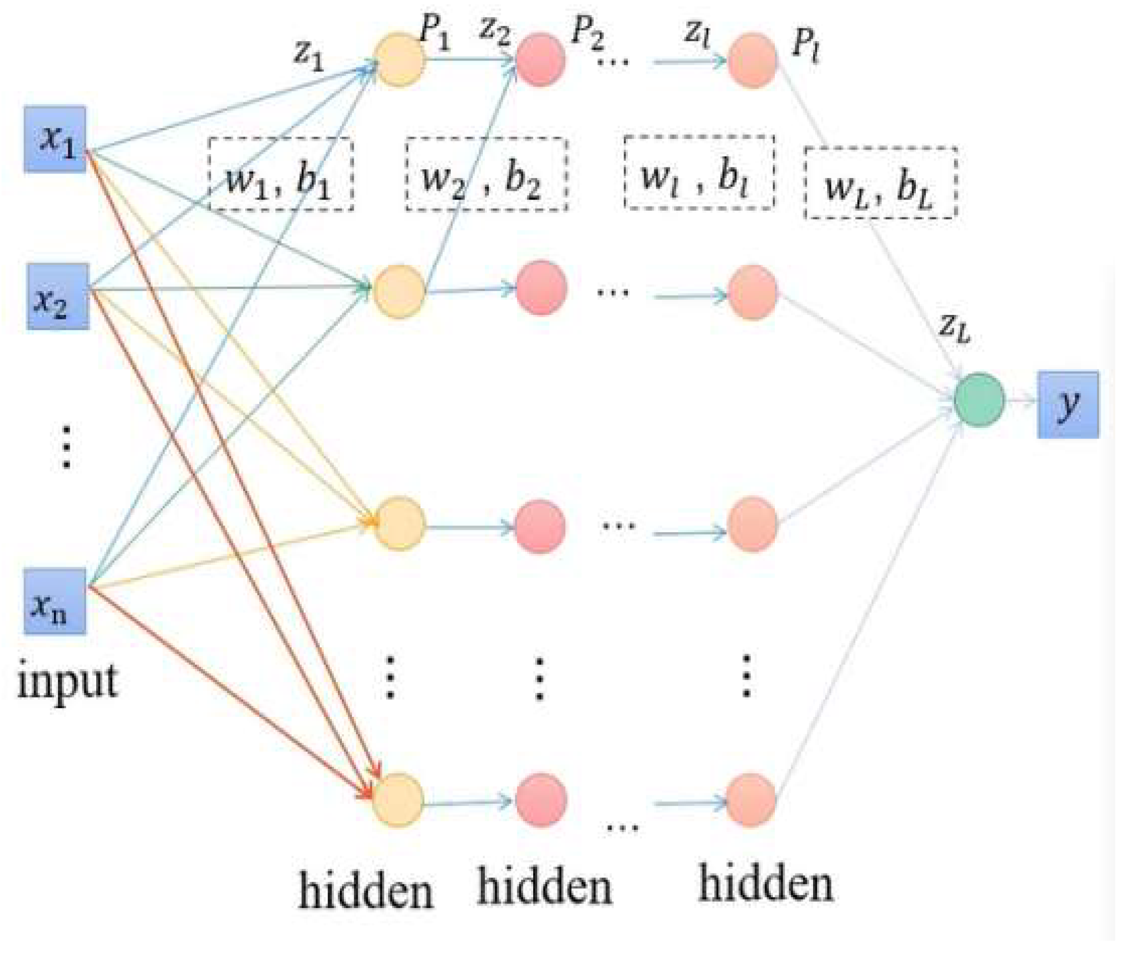
Starting from the input layer, the input of each neuron in the hidden layer is computed, the net input of each layer is computed by weights and bias, and then the activation function is applied to get the output of each layer, and finally the output of the output layer is obtained, and this process is the transfer process from the input to the output in the BP neural network, and the expression of is:
Let be the weight of the neuron connected to , and be the bias of . The net input of each layer is calculated from the weights and biases, and when the activation function of the output layer is the function,we can get:
- (2)
- Gradient descent
BP (Back Propagation) Neural Network is a multi-layer feed-forward neural network that optimizes the network weights by means of a gradient descent algorithm to minimize the prediction error. Gradient descent is an optimization algorithm used to minimize an objective function and is commonly used to train machine learning models.The gradient descent process of BP neural network can be broadly divided into the following steps:
Step 1: Forward propagation: the input data is computed through each layer of the network until the output layer, where the prediction is obtained.
Step 2: Calculate loss: the loss function (e.g. mean square error, cross entropy, etc.) is used to calculate the error between the predicted value and the true value
Step 3: Backpropagation: Starting from the output layer, calculate the gradients of the loss function with respect to the network weights and pass these gradients back to each layer of the network.
Step 4: Weight update: use the gradient and learning rate to update the weights in each layer.
Step 5: Iterative optimization: repeat steps 1-4 until the stopping conditions are met (e.g., the maximum number of iterations is reached or the value of the loss function is below a certain threshold).
Set as data real features, the real value output value is , is the value predicted by the neural network, we ultimately want to get the goal for the real value and through the network to predict the value of the error between the value of as small as possible, the objective function is set to :
For the convenience of derivation, the object is taken out as the target, and then the sum of all the objects is
taken as the final target, and represents the input of the feature:
Figure 1.
Flowchart of multiple implicit layers.
1.2.2. Characterization of Applications in Information Processing
BP (Back Propagation) neural network is a multi-layer feed-forward neural network trained according to the error back propagation algorithm, and is one of the most widely used neural networks. It has the following application properties in information processing:
- (1)
-
Advantages:
- Strong nonlinear modeling ability: the BP neural network can deal with nonlinear relationships and can approximate arbitrary complex function mapping relationships.
- Strong learning and inference ability: through the back propagation algorithm, the model can be trained and learned, thus improving the prediction accuracy of the model.
- Applicable to a variety of tasks: can be applied to classification, regression, clustering and other machine learning tasks.
- Can handle large amounts of data: applicable to large-scale datasets, can be trained and predicted in a shorter period of time.
- (2)
-
Disadvantages:
- Easy to fall into the local optimal solution: the training process of BP neural network relies on the selection of initial parameters, and it is easy to fall into the local optimal solution and difficult to converge to the global optimal solution.
- Long training time: the training process of the model usually requires a large number of iterations, and the training time is long.
- Sensitive to the initial parameters and data preprocessing: the quality of the initial parameters and data preprocessing is highly required, and different parameters and data processing methods may lead to different results.
- Not suitable for all nonlinear systems: for some extreme nonlinear or highly noisy systems, BP neural networks may also fail to achieve good results.
BP neural networks need to be designed with network structure, parameter selection and training tuning according to the characteristics of the specific problem and dataset in practical applications, in order to obtain better training results and generalization performance.
2. Information Data Processing Method Based on UKF-BPNN
From the above analysis of the application of UKF and BPNN in information data detection, it can be seen that the two algorithms have their own advantages and shortcomings in information data fusion processing, and it is difficult to achieve ideal application results by applying them independently in the fusion of information data in complex environments [15]. Therefore, with reference to the advantages of the two algorithms in information data fusion described above, this paper tries to establish the information data fusion model based on UKF-BPNN by combining the two algorithms to improve the detection accuracy of information data in complex environments [16].
2.1. Algorithmic Model
The data collected from the sensors are preprocessed, including cleaning of the data and replacing outliers. In order to obtain the observations for the traceless Kalman filter, the data from each sensor is first named as =(=1,2,3,4 … m) and the variance between the data from each sensor is calculated as (=1,2,3,4 …m).
The variance of sensor =(=1,2,3,4 … m) is:
Where, is the mean value of sensor and is the total number of sensor measurements. With this formula, the variance of each sensor can be calculated and the inverse of the variance between each sensor's data is taken as the weight.
The normalized weights =(=1,2,3.....m),such that the weights for each set of data are multiplied by the observations available for each set of data, and summed according to the weights to obtain the measurements :
The observations are expressed as:
Update the estimate of the state at moment k for moment k-1 and the covariance matrix:
The BP neural network is initialized by assigning an initial value to each connection weight, determining the error function e, the computational precision ε, and the maximum number of learning times M. The function is used as the excitation function, and the set of points is { ,i=0,1,2..k}. When sampling the state quantity at moment , the first point is taken, , and the remaining points are symmetric about mean value.
The results obtained by running the UKF, the inputs to each neuron in the hidden layer are:
The combination can be obtained as the model expression for the application of UKF-based BP neural network multi-sensor data fusion algorithm in multi-sensor data detection as follows
The objective function of the error between the true value and the predicted value is:
In the specific realization process, some practical problems also need to be considered, such as how to choose the appropriate BP neural network parameters, how to adjust the parameters in Kalman filtering, and so on. These issues need to be combined with specific application scenarios for comprehensive analysis and processing.
2.2. Implementation Steps
The process and steps of applying the algorithm presented in this paper in information data fusion are shown in Figure 2
Step 1: Collecting detection bearing data b, pre-processing the sensor data, performing noise reduction, removing outliers and other operations on the data to ensure the quality and accuracy of the sensor data.
Step 2: Substitute the traceless Kalman filter formula to process the preprocessed data and obtain the corresponding state variables. Find the corresponding state estimates and covariance estimates.
Step 3: Perform state estimation and process the state variables using the UKF-BPNN based algorithm to find the fusion value J'.
Step 4: Perform covariance fusion on the estimated state variables to obtain the weighted average of each state variable as the final estimate of the system state, find the error J', and determine whether the iteration needs to be repeated based on whether the threshold of J' exceeds the error. Detect whether the condition is satisfied, output if the condition is satisfied, and continue to iterate if the condition is not satisfied.
3. Examples of Application
3.1. Experimental Platform Establishment
As bearings are an important part of all kinds of equipment, their working condition directly affects the performance of the whole machine. Therefore, it is of great significance to obtain accurate information data in the process of bearing operation in real time, and to realize timely warning of its failure to avoid accidents, in order to enhance the reliability of the equipment and improve its working efficiency. According to the rolling bearing experimental data provided by CWRU University Data Center Laboratory, SKF6205 deep groove ball bearing is used in this paper, and the motor bearing is faulted by electric discharge machining (EDM) [17]. The bearing roller outside diameters ranged from 0.007 inches to 0.040 inches, as measured by micrometer, on the inner raceway, rolling elements (balls), and outer raceway, respectively [18]. The bearings were mounted into the test motor and vibration data was recorded at motor loads of 0 to 3 horsepower (motor speeds of 1797 RPM to 1720 RPM) [19].
3.2. Experimental Step
Referring to the experimental steps described in the literature, the process of processing the information data in this experiment is carried out in the following four steps.
Step 1: Pre-process the bearing failure diameter data, noise reduction and removal of outliers, the vibration data of the motor load =(=1,2,3,4 … m) to obtain its variance , take the inverse of the variance as the weight , after normalization of the weights can be obtained after the observed value.
Step 2: Bring in the state estimation equations and covariance equations to obtain the new bearing failure diameter estimate and covariance estimate .
Step 3: Bring the new bearing state estimate and covariance estimate into the UKF-BPNN operator, which yields the inputs to the neurons in the hidden layer, and substitute them into to obtain the prediction of the bearing error diameter by the joint algorithm.
Step 4: Substitute the error objective function J. If it is smaller than the error threshold, the output is the final data, if it is larger than the error threshold, then return to iteratively run the operator.
3.3. Information Data Processing Results and Analysis
The fusion of UKF and BP neural networks for processing data is feasible and has been shown to be effective in practical applications [20]. This approach can improve the state estimation performance of the system by combining the advantages of both algorithms, especially when dealing with nonlinear and non-Gaussian noise [21,22].
In the experiment, we first measured the fault data values of some bearings in different cases, and then applied different algorithms to fuse the measured data, the prediction effect of various algorithms in the information data is shown in Figure 3, and the bearing prediction error is shown in Figure 4.
From Figure 3, it can be intuitively seen that the data processed by the UKF algorithm has a certain noise reduction effect, but there is a certain deviation from the real value; after the data processed by the joint algorithm of this paper, the prediction results can be closer to the real value of the curve, and the fitting effect is better.
After analyzing the results of the application of a number of data samples, the prediction error of some of the bearings in different cases is plotted as shown in Figure 4, from which it can be seen that the unfiltered data has a larger deviation from the true value; UKF has a certain degree of noise reduction of the data at the same time there is a certain degree of error; after the joint algorithm of this paper, the data is improved and processed by UKF-BPNN, and the generated curves are more closely matched with the true value than the previous two. After this paper's joint algorithm UKF-BPNN improved data processing, the curve generated compared with the first two more closely match the real value, can be more intuitive fitting bearing diameter data.
In information processing, methods combining untraceable Kalman filtering (UKF) and BP neural networks (BPNN) have been widely studied and applied. This combined approach aims to utilize the advantages of UKF in dealing with state estimation of nonlinear systems and the powerful nonlinear fitting capability of BPNN with a view to achieving better performance.Mean Square Error (MSE) is a commonly used measure of the performance of prediction models and is defined as the mean of the sum of the squares of the difference between the predicted value and the actual value. In the UKF-BPNN framework, MSE can be used to evaluate the accuracy of model prediction, which in turn guides model training and parameter tuning. From Figure 5, it can be seen that in UKF-BPNN the mean square error (MSE) of the training and test sets is small.
Confusion Matrix (CM) is a tool for evaluating the performance of a classification model that shows the relationship between the results predicted by the model and the actual labels. The Confusion Matrix provides the performance of the model on the training data, which helps us to understand the model overfitting as well as to find out which categories are easily confused by the model, so that we can distinguish these categories by further feature engineering, which guides us to adjust the parameters of the model, such as the regularization parameter of the Support Vector Machines, in order to improve the performance of the model.
According to Figure 6, it can be seen that the confusion matrix shows that the prediction results of certain categories all reach more than 90%, which shows that the accuracy of the matrix is high under this algorithm.
The test data confusion matrix shows how the model performs on unseen data, which is a key metric for evaluating the model's generalization ability. The test set is usually independent of the training set, so the test data confusion matrix provides an estimate of the model's likely performance in real-world applications. By analyzing the test data confusion matrix, patterns of model prediction errors can be identified, which can help to further improve the model. In some cases, the performance of the model can be improved by adjusting the classification thresholds, and the confusion matrix for test data can help us determine the optimal threshold.
According to Figure 7, it can be seen that the test data confusion matrix in for data fitting and the real value fitting degree is higher, that is, the fusion algorithm introduced in this paper is more feasible for data processing.
Overall, the confusion matrix is an important tool for evaluating the performance of classification models, which not only helps us understand how the model performs on training and test data, but also guides us in model optimization and improvement.
By analyzing the application of the three algorithms of UKF, BPNN and UKF-BPNN in the case, the average absolute error and mean square error of the information data processed by different algorithms can be obtained, as shown in Table 1. From the table, it can be seen that: the fit of UKF -BPNN algorithm for the bearing failure diameter, compared with the single UKF and BP algorithm function of the average absolute error and mean square error is smaller, that is, the algorithm of this paper's prediction estimate is more accurate and reliable.
4. Conclusion
In engineering practice, information detection systems work in complex environments, so their information data measurements are subject to multiple factors, which bring unpredictable measurement errors. In this paper, through the study of untraceable Kalsman (UKF) and BP neural network (BPNN), it is found that in the detection and processing of information data: UKF has strong nonlinear estimation ability, and BPNN has strong automatic learning ability. The complementary advantages of both in information data processing are realized by combining UKF and BPNN. The information data fusion model based on UKF-BPNN is established and applied to the detection of information data in complex environments. UKF is first used to provide state estimation as the input to the BP neural network, and then the J function that meets the error threshold is derived, so that the predicted value can maximally fit the real value, which greatly improves the detection accuracy of information data in complex environments. Through its application experiments in the measured values of motor bearings after electrical machining, it proves the application advantages of the method in estimating accuracy. A new integrated method is provided for the field of nonlinear state estimation and machine learning, which helps to solve the estimation and control problems in complex systems.
Acknowlelgments
This project was supported by the National Natural Science Foundation of China [grant numbers 51878005 and 51778004] and the Anhui Provincial Education Commission Foundation, China [grant number KJ2020A0488].
References
- Wu, X. Analysis of modern mechanical design and manufacturing process and precision machining technology [J]. China Equipment Engineering 2023, 520, 109–111. [Google Scholar] [CrossRef]
- Zhou, Y.; Hu, J.; Zhao, Y.; et al. Vehicle target tracking based on Kalman filter improved compressed perception algorithm[J]. Journal of Hunan University (Natural Science Edition) 2023, 50, 11–21. [Google Scholar] [CrossRef]
- Yang, Z.; Li, Y.; Wu, G. Research on denoising technique of IMU sensor based on traceless Kalman filter and wavelet analysis[J]. Modern Electronic Technology 2024, 47, 53–59. [Google Scholar] [CrossRef]
- Xie, K.; Qin, P. Research on the extrapolation algorithm of gun position detection radar based on Doppler information[J]. Journal of Ballistics 2018, 30, 53-58+76. [Google Scholar] [CrossRef]
- ZHANG Yu, YAO Yao, LIU Rui,et al. Joint estimation method of SOC/SOP for all-vanadium liquid-flow battery based on adaptive traceless Kalman filtering and economic model predictive control[J/OL].Energy Storage Science and Technology,1-13[2024-07-31]. [CrossRef]
- Zhang, C.; Wang, L.; Kong, X. A hemispherical resonant gyro temperature modeling compensation method based on KPCA and data processing combined method neural network[J]. Journal of Zhejiang University (Engineering Edition) 2024, 58, 1336–1345. [Google Scholar] [CrossRef]
- DONG Yi-Han,ZENG Sen,ZHOU Xiang. Optimization of BP neural network based on genetic algorithm for RC column skeleton curve prediction[J]. China Water Transportation, 2024, 24(07) :34-36. Journal, 2024, 45(08): 94-99+106. [CrossRef]
- Yanqiang Duan. Coal rock identification error analysis based on BP neural network optimization algorithm[J]. Energy and Energy Conservation, 2024, 4-7. [CrossRef]
- Nie, J.L.; Qin, Y.; Liu, F. Adaptive UKF-based BP neural network and its application in elevation fitting[J]. Surveying and Mapping Science 2007, 120-122+208. [Google Scholar] [CrossRef]
- T. Haarnoja, A. Ajay, S. Levine, and P. Abbeel, “Backprop KF: Learning discriminative deterministic state estimators,” in Advances in Neural Information Processing Systems, 2016, pp. 4376–4384.
- C.-F. Teng and Y.-L. Chen, “Syndrome enabled unsupervised learning for neural network based polar decoder and jointly optimized blindequalizer,” IEEE Trans. Emerg. Sel. Topics Circuits Syst., 2020. [CrossRef]
- Revach, G.; Shlezinger, N.; Ni, X.; Escoriza, A.L.; van Sloun, R.J.; Eldar, Y.C. KalmanNet: Neural network aided Kalman filtering forpartially known dynamics. IEEE Trans. Signal Process. 2022, 70, 1532–1547. [Google Scholar] [CrossRef]
- X. Ni, G. Revach, N. Shlezinger, R. J. van Sloun, and Y. C. Eldar, “RTSNET: Deep learning aided Kalman smoothing,” in Proc. IEEE ICASSP, 2022. [CrossRef]
- Shlezinger, N.; Eldar, Y.C.; Boyd, S.P. Model-based deep learning:On the intersection of deep learning and optimization. arXiv 2022, arXiv:2205.02640. [Google Scholar] [CrossRef]
- M. B. Matthews. A state-space approach to adaptive nonlinear filteringusing recurrent neural networks. In Proceedings IASTED Internat. Symp. Artificial Intelligence Application and Neural Networks, pages 197–200, 1990.
- Puskorius, G.; Feldkamp, L. Decoupled Extended Kalman Filter Training of Feedforward Layered Networks. IJCNN 1991, 1, 771–777. [Google Scholar] [CrossRef]
- Deng, S.; Chang, H.; Qian, D.; Wang, F.; Hua, L.; Jiang, S. Nonlinear dynamic model of ball bearings with elastohydrodynamic lubrication and cage whirl motion, influences of structural sizes, and materials of cage. Nonlinear Dyn. 2022, 110, 2129–2163. [Google Scholar] [CrossRef]
- Bovet, C.; Linares, J.-M.; Zamponi, L.; Mermoz, E. Multibody modeling of non-planar ball bearings. Mechanics & Industry 2013, 14, 335–345. [Google Scholar] [CrossRef]
- Xiu C, Su X, Pan X. Improved target tracking algorithm based on Camshift. In: 2018 Chinese control and decision conference (CCDC), Shenyang, China, 2018, pp.4449–4454. Piscataway, NJ: IEEE. [CrossRef]
- Hsia K, Lien SF, Su JP. Moving target tracking based on CamShift approach and kalman filter. Int J Appl Math Inf Sci 2013; 7: 193–200. [CrossRef]
- Qu, S.; Yang, H. Multi-target detection and tracking of video sequence based on kalman_BP neural network. Infrared Laser Eng 2013, 42, 2553–2560. [Google Scholar]
- ReganChai. BP Kalman Fusion Prediction. Online Referencing. https://github.com/ReganChai/BPKalman-FusionPrediction (accessed 21 April 2018).
Figure 2.
UKF -BPNN algorithm flow.
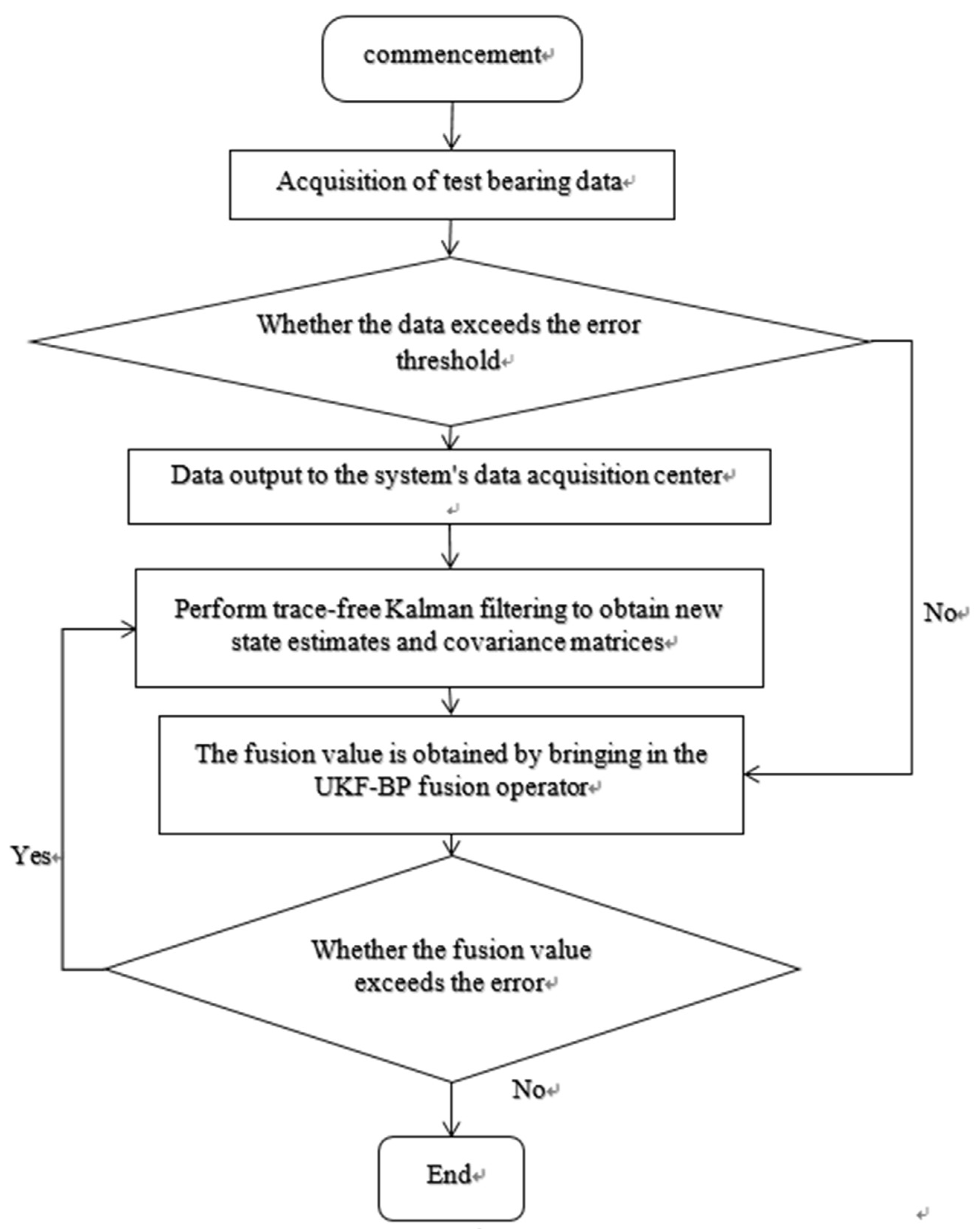
Figure 3.
Comparison of the prediction results of some bearings under different algorithms.
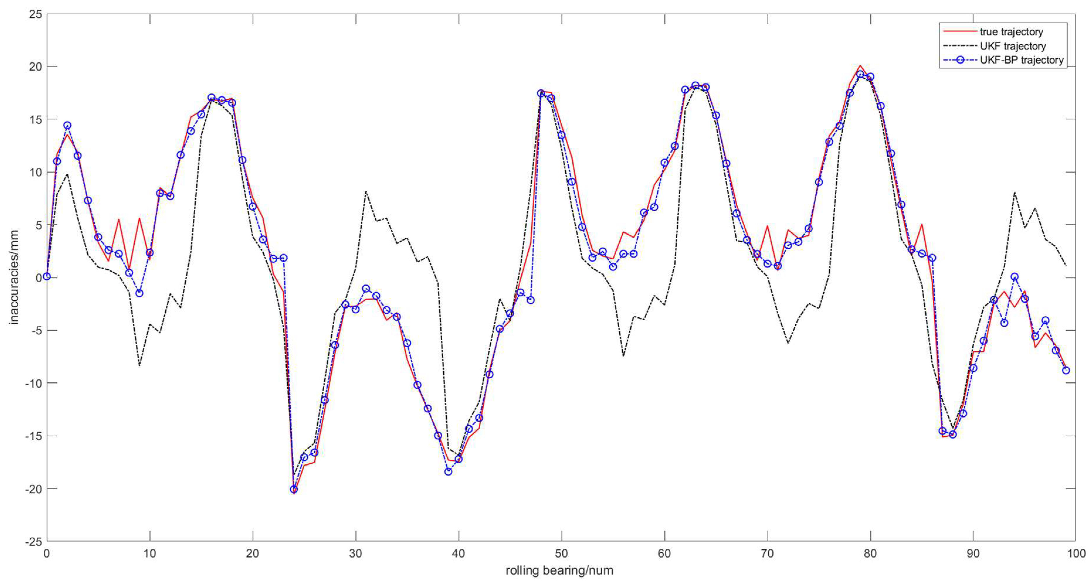
Figure 4.
Comparison of prediction errors of some bearings in different cases.
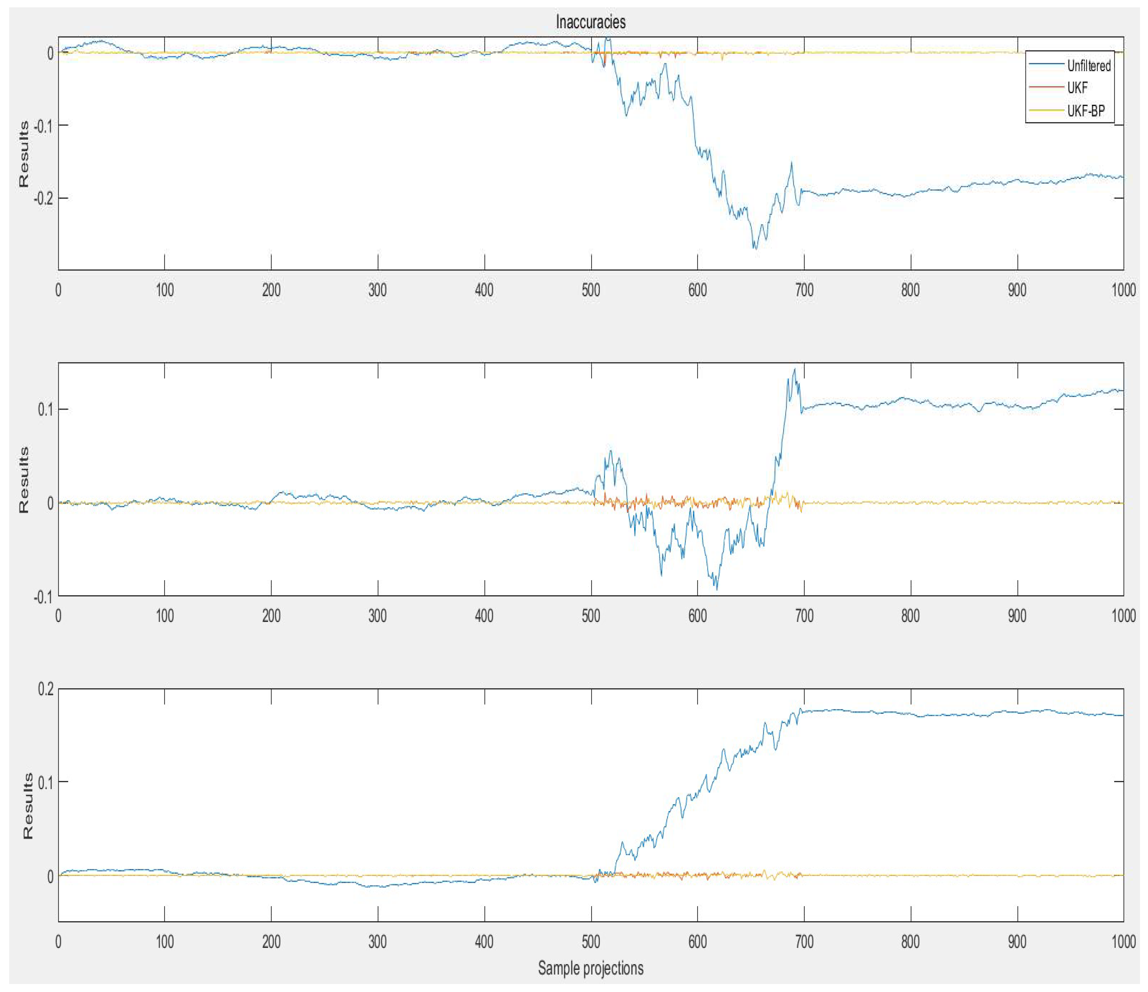
Figure 5.
Mean square error of UKF -BPNN.
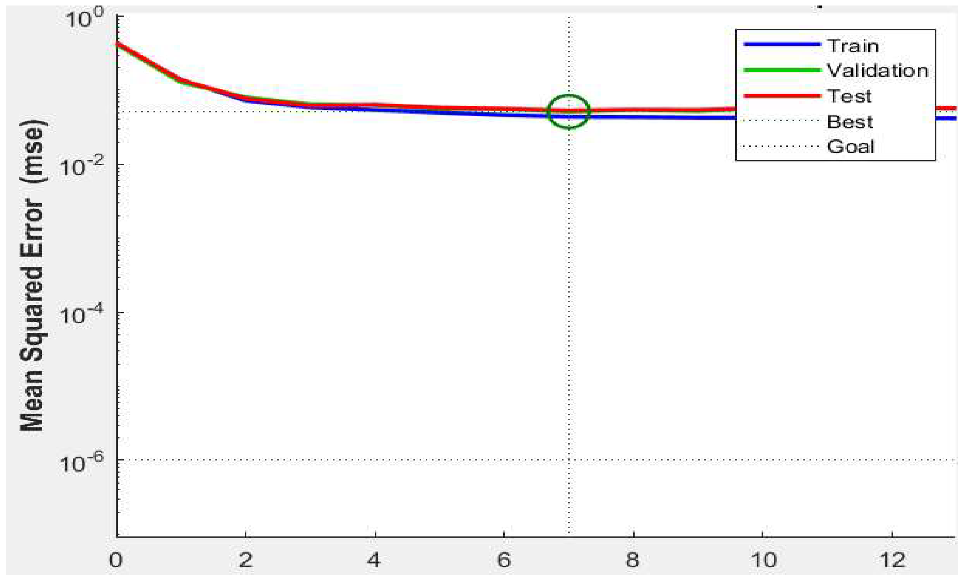
Figure 6.
Confusion Matrix for Train Data.
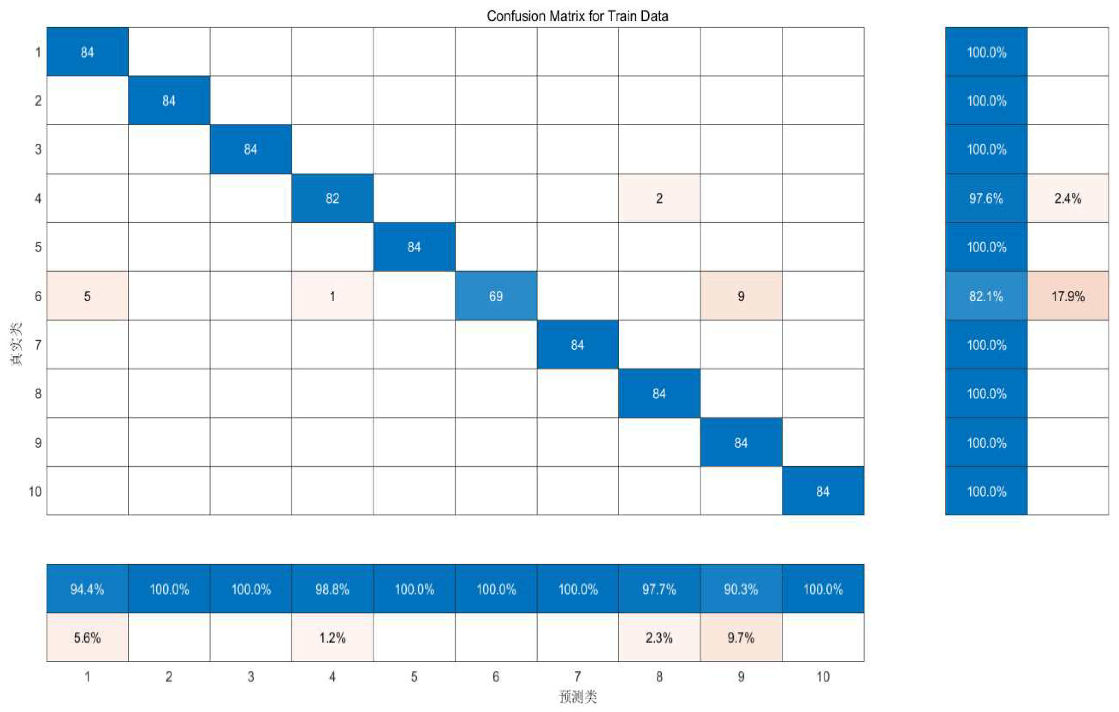
Figure 7.
Confusion Matrix for Test Data.
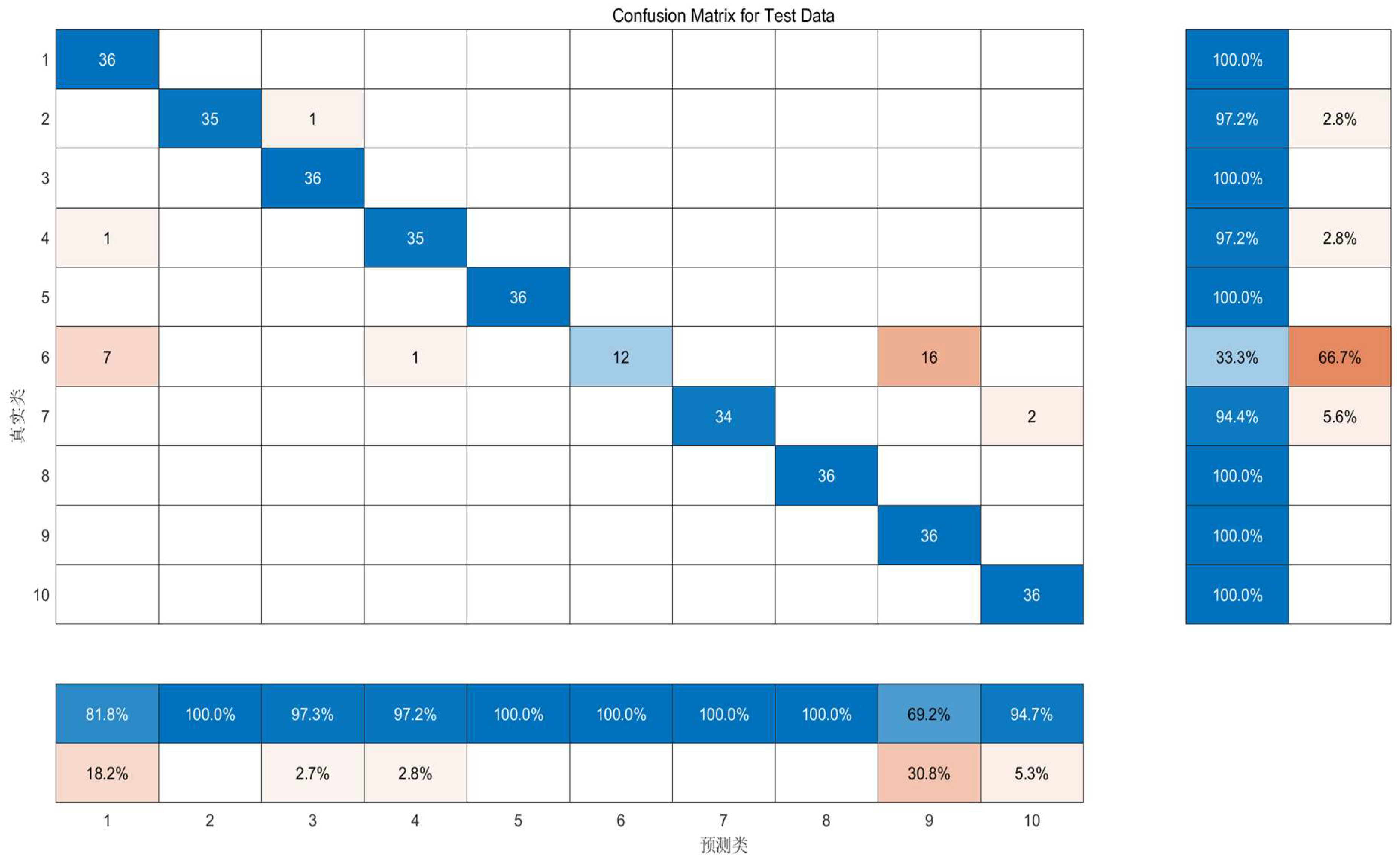

Table 1.
Mean absolute and mean square errors for multiple filters.
| Arithmetic | MAE | MSE |
| UKF | 0.6325 | 0.0693 |
| BPNN | 0.4843 | 0.0773 |
| UKF -BPNN | 0.1132 | 0.0512 |
Disclaimer/Publisher’s Note: The statements, opinions and data contained in all publications are solely those of the individual author(s) and contributor(s) and not of MDPI and/or the editor(s). MDPI and/or the editor(s) disclaim responsibility for any injury to people or property resulting from any ideas, methods, instructions or products referred to in the content. |
© 2024 by the authors. Licensee MDPI, Basel, Switzerland. This article is an open access article distributed under the terms and conditions of the Creative Commons Attribution (CC BY) license (https://creativecommons.org/licenses/by/4.0/).
Copyright: This open access article is published under a Creative Commons CC BY 4.0 license, which permit the free download, distribution, and reuse, provided that the author and preprint are cited in any reuse.


