
Submitted:
29 October 2024
Posted:
30 October 2024
You are already at the latest version
Abstract
Objective:
This study explores the impact of public policies that promote social equity and rights to nature on subjective well-being (SWB). The focus is on how sustainability policies, particularly on environmental protection and poverty reduction, have influenced life satisfaction in Ecuador.
Design/methodology/approach:
The research uses ordinal logistic regression models to analyze data from the National Survey of Employment, Unemployment and Underemployment of Ecuador. Life satisfaction is the dependent variable, while independent variables include income, education, job satisfaction, concern for the environment, and regional differences.
Findings:
The results indicate that the implementation of public social investment policies increases life satisfaction,
particularly in regions such as the Coast. After the implementation of the policy, income, higher education, job satisfaction, and concern for the environment were associated with higher levels of subjective well-being. However, disparities persist, with lower life satisfaction among indigenous groups, women, the elderly, and those living in poverty.
Originality/value:
This study provides valuable insights into the relationship between sustainable policies and subjective well-being, highlighting Ecuador's unique constitutional framework. It offers lessons for other developing nations seeking to balance social equity, economic growth, and environmental sustainability in pursuit of improving overall quality of life.
Keywords:
subjective well-being (I31)
; sustainability (Q56)
; poverty (I32)
; inequality (D63)
; environmental policy (Q58)
1. Introduction
Studies that establish a relationship between sustainability and subjective wellbeing have become increasingly relevant in the study of social policies and how they impact people's quality of life. Ecuador presents a unique case with its 2008 Constitution, which enacts social equity and poverty reduction, but also recognizes the rights of nature, an unprecedented concept in this era. This study aims to explore how these disruptive constitutional principles have influenced the life satisfaction of Ecuadorians, using data from before and after the implementation of the analysed Constitution.
The 2008 Ecuadorian Constitution marked an unprecedented shift towards a more sustainable development model, this mandate is characterized by environmental protection and equitable redistribution of resources. The orientation of this new mandate was to promote benefits mainly for the most vulnerable. Through this study we want to examine life satisfaction from the perspective of sustainability, additionally we intend to identify whether these policies have managed to improve the quality of life in different demographic groups and different regions of Ecuador.
To achieve this, we apply ordinal logistic regression models to data from 2007 and 2014, which represent the period before and after the promulgation of the Constitution. The study employs several factors that affect life satisfaction, among them: income, education, job satisfaction and finally, concern for the environment, at the same time considering the regional disparities between each of the regions of the country (Coast, Center and East).
This comparative analysis not only establishes the effects of the Constitution on subjective wellbeing, but also provides insights into considerations for the design of sustainable policies that seek to improve life satisfaction in other developing nations. The Ecuadorian experience provides valuable lessons for countries seeking to balance economic growth, social equity and environmental sustainability in their quest for a better quality of life for all their citizens.
Subjective wellbeing (SWB) has emerged as an important field of study in the field of psychology and this in turn to other fields of knowledge, the economic sciences being no exception. To process these indicators, the starting point is how people evaluate their own lives. This evaluation is based on cognitive judgments, but also on how they define their affective relationships either as happiness or sadness (Gataūlinas & Banceviča., 2014). The concept of SWB is considered multidimensional as it usually includes components such as life satisfaction, positive affect and negative affect. Research such as Diener's (1984) highlights that SWB includes both reflective cognitive appraisals and affective reactions to life events, making it a comprehensive measure of individuals' overall quality of life.
Within the literature, SWB can be influenced by elements such as socioeconomic status, social networks, and personal competence. For example, Pinquart and Sorensen (2000) established that the aforementioned elements significantly influence subjective well-being in adults. On the other hand, George K., (2010) established that the role of social support is preponderant, that is, people who receive more emotional support tend to report higher levels of life satisfaction This suggests that both social and economic contexts play a vital role in shaping individuals' perceptions of their well-being. (Scorsolini & Santos., 2010).
Additionally, establishing a relationship between income and well-being has been the subject of much debate. The “wealth-happiness paradox” argues that, beyond a certain point, an increase in income does not necessarily lead to a corresponding increase in happiness. Although indicators such as GDP is often a good proxy for SWB, income inequality has been shown to reduce average SWB across societies. These results suggest that economic factors are important, but they are not the sole determinants of well-being in its full context. (George., 2010).
It is not only individual factors that can affect subjective well-being. It is social and political implications that can affect their well-being. That is why states are considering more this field of subjective well-being incorporating it in their agendas when formulating policies, there are several programs such as the “National Wellbeing Measurement Program” in the United Kingdom that employ SWB indicators in structuring social policies (Deeming, C., 2013). This integration of well-being signals the importance and relevance it gains within the political discourse.
Cross-national research has generated relevant information on how social contexts affect social welfare. Among the factors established in such studies we have: economic development, democratization and even social tolerance considered as significant predictors for happiness (Pacheco-Jaramillo, 2023). Although it is necessary to deepen with analyses that consider specific ages, based on older adults to have a better understanding of how these factors interact as a function of age (George, 2010). But it is also necessary to establish their relationship in cultural contexts, because according to (Jun, K., 2015) cultural beliefs and values significantly affect people's perception of well-being.
It is necessary to conceptualize happy life expectancy (HLE) which is based on the measurement of the number of years that people can expect to live happily. Studies in both the United States and the Netherlands show that HLE has increased over time, suggesting improvements in both life expectancy and the quality of those years (George, 2010).
Considering more factors in these analyses provides a broader understanding of SWB where both longevity and happiness converge. To this end, various scales and methodological tools have been established for the measurement and evaluation of vital well-being. Prominent among them are, for example, The Satisfaction with Life Scale (SWLS) and the Positive and Negative Affect Schedule (PANAS) (Gataūlinas & Banceviča., 2014) (Lindert et al., 2015). Although it is necessary to consider cultural and gender contexts in order to ensure its universal applicability (Lindert et al., 2015). This is crucial when making comparisons between countries and diverse populations.
Subjective well-being is a multidimensional concept influenced by various factors, such as social support, economic conditions and even cultural contexts. Although significant progress has been made in understanding these influences, there are still many gaps in knowledge about the interaction of the different variables that shape people's perception of well-being. Considerations for measuring the fullness of life must be informed by the applicability of the tools and their measurement in different cultural contexts.
2. Structure of the Data
In Ecuador, there is a higher concentration of poverty among indigenous people in the Eastern areas. With the econometric models, I will test whether the Eastern people are more satisfied than those in other regions controlling for other variables that affect wellbeing. Thus, this aspect of the study explores the regional disparities further. Consequently, I also want to determine through the econometric models which region has people who are more satisfied. This is crucial to understanding the regional disparities and identifying which region has higher levels of life satisfaction.
Dummy variables and categorical variables are created for the regions (Eastern, Coast, and Central regions and urban/rural areas), age, gender, ethnicity, education, job satisfaction,1 income,2 poverty, extreme poverty, marital status, and environmental concern (see Table 1). The information about poverty and extreme poverty is related to the question in the survey about the head of the household’s living conditions.2
I used the 2014 mean as a reference to classify life satisfaction into three categories. High levels of life satisfaction were classified as greater than the mean of life satisfaction plus one standard deviation (SD) (9–10 points on the Likert scale), moderate life satisfaction was classified as a value falling within one SD above and below the mean of life satisfaction (6–8) and low life satisfaction was classified a value more than one SD below the mean (5)4. Thus, the three classifications of satisfaction are: unsatisfied, satisfied and very satisfied.
Associated with the economic variables, income data is collected in the surveys in both years. The way this data was collected is different for 2007 compared to 2014. For instance, in 2007, the income of the head of the household was represented by monthly wages, and in 2014, income was represented by net earnings per year6 of the head of the household in the last year. Thus, the income variable is not able to be compared across both periods. However, I will analyse how income affects life satisfaction in each year of analysis.
Related to the sample by region, the ENEMDU 2007 and ECV 2014 surveys have a different sample size, but they have the same questions in the perception of life section. For example, the ECV survey collected more information from the population in the Eastern area in 2014 (15.37%) than ENEMDU in 2007 (4.5%). The ECV 2014 survey increased the sample in comparison to ENEMDU 2007. Also, the ECV 2014 survey was created to be more representative at the national, urban, and rural levels, with four natural regions, 24 provinces, nine planning zones and four self-represented cities (Quito, Guayaquil, Cuenca, and Machala) included (ECV 2014). Additionally, the Ecuadorian National Institute of Statistics and Censuses (INEC)7 included topics in the ECV 2014, such as psychosocial wellbeing, perception of the standard of living, social capital, citizen security, use of time and good environmental practices. For instance, in terms of regional characteristics, the ENEMDU survey gathered more information about the condition of people in the Eastern region where there is a greater concentration of poverty (Molina et al. 2016). The increase in the sample size of the Eastern region from 2007 to 2014 was due to the change of the collection methodology to cover more geographic areas. However, as noted previously, the questions in both surveys were the same, and were addressed to the same groups of people (heads of households). Most heads of households in Ecuador are males: the ENEMDU survey had 78.1% of male heads of households in 2007 and the ECV survey had 75.51 in 2014.
The main characteristics of the sample in terms of age groups are that the younger group (13/14–34 years old) was fell more often into the “very satisfied” category than other age groups in 2007, and the older group (65 years and above) was more unsatisfied than the other groups. These results are tested within the econometric models.
In terms of tertiary education, I have created a dummy variable to identify who has a post-school studies, such as university or superior institute studies (non-university post-secondary school), and who does not have such a qualification. According to the literature review, people who have more years of study are more satisfied with life than others. High education was shown to have a positive impact on Ecuadorian wellbeing. However, a high level of education has been found to have a stronger association with wellbeing in low-income countries such as Ecuador (Miranti et al. 2017).
In addition, subjective wellbeing within the categories of marital status is tested through the following categories: married or in a de facto union; divorced, separated, or widowed; and single. According to Nicola, Bravo, and Sarmiento (2018), in Ecuador people who are married or in a de facto union have greater wellbeing than single people, or those who are separated or divorced. These results are also supported by European, American, Asian and Latin American studies (Steptoe, Deaton, and Stone 2015).
Thus, a dummy variable of environmental concern was created, where one (1) represents an excessive, very, or moderate concern and zero (0) represents low or no concerns.
Table 2 shows the characteristics of the variables used in 2007 and 2014 to create the models.
3. The Economic Model
The economic theory on which this research is based hypothesises that the new constitution increased life satisfaction for Ecuadorians, taking all other variables into account. Thus, one expects these explanatory variables to have a positive effect on life satisfaction (used as a measure of subjective wellbeing). (see Table 2).
The econometric model will show the association between subjective wellbeing in Ecuador and the implementation of the 2008 Constitution.
To produce more meaningful results, “unsatisfied” is used as the base in the ordinal logistic model in STATA, to compare with “satisfied” and “very satisfied” responses, ordered from 0 to 2.
The economic model is expressed in this way:
3.1. Equation 1, Economic Model
The explanatory variables –regions, area, age, gender, job and ethnicity – and their correlations will be related to life satisfaction. This specification will allow the model to test whether life satisfaction is associated to the 2008 Constitution.
3.2. Correlations between the Variables
Before conducting a regression, it is important to understand the underlying data. While the distribution of the variables has already been examined, looking at correlations between them will be the first indicator of whether multicollinearity exists in the regression. This section shows the correlation matrix between all variables of the model in 2007 and 2014.
3.3. Correlation between the Variables in 2007
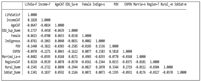
When we look at a correlation matrix of the 2007 data, the relevant results are that living in the Coast and the Central regions, income (above the mean), job satisfaction and education have a positive correlation with life satisfaction. Living in the Eastern region, living in rural areas, age (above 55 years old), poverty and extreme poverty, being a female, being indigenous, and being married have a negative correlation with life satisfaction. There are clear disparities of gender, ethnicity and income in Ecuador. Also, in Latin America more broadly, poverty and inequality among females and indigenous people is higher than for males and non-indigenous people (Pérez 2004).
Looking at the correlations from high to low, female and married have the highest correlation (0.49); then, income and poverty (-0.44) have the next highest (negative) correlation, followed by tertiary education and income (0.43), and poverty and living in rural areas (0.33).
The rest of the variables have weak correlations among each other, suggesting multicollinearity will not be a problem in the model. Although it is difficult to define what represents a high, moderate or weak correlation between two variables, Hayes (2021) suggests that correlations less than 0.30 are weak, those between 0.31 and 0.69 are moderate, and those greater than 0.70 are high. None of the correlations identified in Table 3 are high enough, nor are there enough of them, to cause problems with multicollinearity.
Table 3. Correlation table of the variables in 2007.
Source: Author’s summary STATA.
3.4. Correlation between the Variables in 2014
In the 2014 data, as shown in Table 4, life satisfaction has a positive relationship with the Coast and Central regions relative to the Eastern region, and net income (above the mean), education, and environmental concern. Also, there is a positive relationship between indigenous and rural areas. It was noted that poverty is higher in Ecuadorian rural areas where there is the highest concentration of indigenous people, and that indigenous women are much more vulnerable due to the lack of household income and access to jobs. In the Eastern region there is also a higher proportion of the population living in rural areas in comparison to the other regions.
Living in the Eastern region, being older, living in a rural area, being a female, being a female, being part of an indigenous group, being poor, and being married have a negative correlation with life satisfaction.
As in 2007 data, all the variables mentioned above have a weak correlation in the 2014 model, again suggesting multicollinearity will not be a problem for this year.

Table 4.
Correlation table of the variables in 2014.
| LS | Eastern Dumm | Rural | Mingas | Caring | Disabi | Net Income | Age | Ter EDU | Female | Indigen | Po- verty |
Envi- ronme |
Re- ligion |
Ma- rried |
|
|---|---|---|---|---|---|---|---|---|---|---|---|---|---|---|---|
| LS | 1.00 | ||||||||||||||
| Eastern D | -0.03 | 1.00 | |||||||||||||
| Rural | -0.08 | 0.20 | 1.00 | ||||||||||||
| Mingas | -0.03 | 0.05 | 0.19 | 1.00 | |||||||||||
| Caring | 0.01 | 0.06 | -0.03 | 0.01 | 1.00 | ||||||||||
| Disabi | -0.02 | -0.01 | 0.00 | -0.02 | 0.02 | 1.00 | |||||||||
| Net income | 0.07 | -0.03 | 0.09 | 0.01 | -0.03 | -0.02 | 1.00 | ||||||||
| Age | -0.06 | -0.13 | 0.11 | -0.04 | -0.32 | 0.03 | 0.01 | 1.00 | |||||||
| Ter EDU | 0.09 | -0.05 | -0.23 | -0.06 | 0.04 | -0.01 | 0.06 | -0.09 | 1.00 | ||||||
| Female | -0.09 | -0.06 | -0.06 | -0.05 | 0.10 | 0.05 | -0.15 | 0.03 | -0.05 | 1.00 | |||||
| Indigen | -0.11 | 0.29 | 0.32 | 0.29 | 0.04 | -0.01 | -0.06 | -0.06 | -0.11 | -0.04 | 1.00 | ||||
| Poverty | -0.15 | 0.09 | 0.22 | 0.03 | 0.00 | 0.04 | -0.13 | 0.09 | -0.18 | 0.09 | 0.14 | 1.00 | |||
| Environ | 0.06 | -0.01 | -0.15 | -0.03 | 0.05 | 0.00 | 0.04 | -0.10 | 0.14 | -0.03 | -0.12 | -0.13 | 1.00 | ||
| Religion | -0.02 | -0.02 | 0.03 | -0.06 | 0.03 | 0.01 | 0.02 | -0.04 | -0.01 | 0.01 | -0.06 | 0.02 | -0.01 | 1.00 | |
| Married | -0.08 | -0.05 | -0.07 | -0.06 | 0.00 | 0.04 | -0.14 | 0.07 | -0.01 | 0.61 | -0.08 | 0.08 | -0.03 | 0.03 | 1.00 |
Source: Author’s summary STATA.
All the analysis presented so far has been bivariate, and the other variables may be affecting any of these correlations. A rigorous analysis uses regression to identify the impact of life satisfaction controlling for all other variables.
3.5. Using Ordered Logit Regression
Ordered logit models are used to estimate the relationships between an ordinal dependent variable and a set of independent variables (StataCorp 2019; Lu 1999). An ordinal variable is a variable that is categorical and ordered, for example, “unsatisfied”, “satisfied” and “very satisfied”, which could indicate the current life perception of a head of household. Very satisfied has a higher order than satisfied and satisfied has a higher order than unsatisfied.
The ordered logit regression fits the model since I am comparing the three ordered categories of life satisfaction. Also, ordered logit regression represents the results more clearly. Ordinal logit coefficients represent changes in the log-odds for a one-unit increase in the independent variables. If the x variable is a dummy variable, we can exponentiate its coefficient β to get an “adjusted odds ratio”.
3.6. R-Square and Pseudo R-Square in Regression Models
The use of R-square has been debated recently in the political science literature. Hagquist and Stenbeck (1998) discussed that R-square is only a measure of the degree of agreement between the effect of the model on the result. According to Hu, Shao, and Palta (2006, 848), “there is no clear interpretation of the pseudo-R2s in terms of variance of the outcome in logistic regression... the pseudo-R2s for a given data set are point estimators for the limiting values that are unknown”. Also, the McFadden statistic in logit models points to a low degree of explanation of the control variables; for example, in ordinal or categorial logit, the pseudo-R2 has a limited interpretation9 (Soukiazis and Ramos 2016).
After fitting the logistic regression model, we want to know how well we can predict the dependent variable, which is life satisfaction. A model can fit the data well but do a poor job of predicting, or a model can predict the outcome well but does not fit well (low pseudo R-square).
3.7. The Models
Identifying the determinants of life satisfaction after the implementation of the new constitution is the priority in this research to comparing life satisfaction 2007 and 2014. The models include a set of predictor variables that, according to the literature and the descriptive findings of this study, are the determinants of life satisfaction.
I use statistical software (STATA) to correct multicollinearity and heteroskedasticity problems in all econometric models. Thus, I obtained a better estimate of the results (the goodness of fit).
3.8. The 2007 Model
The full model adds the regional dummy variables to the intermediate model. This will allow us to understand the influence of the regions – the Coast, Central and Eastern – on life satisfaction. In this case, the model is expressed by:
3.9. Equation 2, Full Model
Through this equation or model, I will show the likelihood of being more satisfied, rather than less satisfied, because of a change in all explanatory variables.
3.10. The Econometric Model with the 2007 Dataset: Life Satisfaction, Regions and Control Variables
The full model adds all variables, including regions. Significant variables and then the odds ratios are presented below (see Table 5).
A test for multicollinearity confirmed a variance inflation factor VIF of 1.46 (mean) (see appendices). Thus, no problems of multicollinearity were found in the full model for 2007.
Table 5. Controlled, and demographic variables with regions in 2007 (odds ratios).
Source: Author’s summary STATA. ***statistically significant at the 1% level (<0.001); **statistically significant at the 5% level (<0.05).
The pseudo-R2 in the full model is also low: 0.039. When regions are added to the model, only the Coast region and living in rural areas are significant. The impact of age groups is significant, compared with the youngest group. All income categories, job satisfaction, poverty, gender, ethnicity, tertiary education, and marital status are also significant.
3.11. Interpretation of the Estimates of the Model 2007
The odds ratio of 1.17 for the Coast region means that living in the Coast is associated with 17 per cent greater odds of being in a higher rather than a lower category of LS. However, the odds ratio of 0.743 for rural/urban areas, means that living in rural areas is associated with 25.7 per cent lower odds of being in a higher rather than a lower category of LS.
The odds ratios of 0.89 for those aged between 35 and 44 years means this age group is associated with 11 per cent lower odds of being in a higher rather than a lower category of LS. The odds ratios of 0.813 for the age group of 55–64 years means it is associated with 18.7 per cent lower odds of being in a higher rather than a lower category of LS, and 0.679 for the 65+ age group means it is associated with 32.1 per cent lower odds of LS. Younger people aged between 13 and 34 years old are the basis of the age range analysis.
Life satisfaction decreases as age increases in 2007 for both the “satisfied” and “very satisfied” ranges. Ecuador, a developing country and as a part of Latin America, shows a progressive decrease in wellbeing with age, in contrast with developing countries, where lower levels of wellbeing are evident in the age groups below 65 years (Steptoe, Deaton, and Stone 2015).
The odds ratio of 1.341 for income in the USD 323–747 range means that this category of income is associated with 34.1 per cent greater odds of being in a higher rather than a lower category of LS. The odds ratios of 1.512 for income in the USD 748–1070 range means that this category is associated with 51.2 per cent greater odds of being in a higher rather than a lower category, and the odds ratio of 1.611 for income of more than USD 1070 is associated with 61.1 per cent greater odds of being in a higher rather than a lower category of LS relative to the income base (lower than USD 322).
The odds ratio of 1.517 for job satisfaction means that being satisfied with a job is associated with 51.7 per cent greater odds of being in a higher rather than a lower category of LS. The odds ratio of 1.581 for tertiary education indicates that each additional year of education (after 12 years of formal education) is associated with 58.1 per cent greater odds of being in a higher rather than a lower category of LS.
However, the odds ratios of 0.801 for poverty means that being poor is associated with 19.9 per cent lower odds of being in a higher rather than a lower category of LS and the odds ratios of 0.826 for gender means that being a female is associated with 17.4 per cent lower odds of being in a higher rather than a lower category of LS. For ethnicity, being indigenous is associated with 25.4 per cent lower odds of being in a higher rather than a lower category of LS.
The odds ratio of 0.831 for being divorced or separated means that this marital status is associated with 16.9 per cent lower odds of being in a higher rather than a lower category of LS relative to being married or in a de facto union. Also, an odds ratio of 0.791 for being single means that single status is associated with 20.9 per cent lower odds of being in a higher rather than a lower category of LS relative to being married or in a de facto union.
3.12. The 2014 Model: Determinants of Life Satisfaction in 2014 (Regions, and Control Variables)
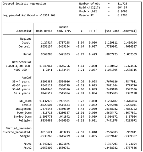
The full model includes all controlled variables; specifically, regions are added into this model. The results from this model are shown in Table 6.
A test for multicollinearity confirmed a variance inflation factor VIF of 1.76 (mean) (see appendices). Thus, we no problems of multicollinearity were found in the full model for 2014.
Table 6. The 2014 model: Determinants of life satisfaction in 2014 (regions, and controlled variables).
Source: Author’s summary STATA. ***statistically significant at the 1% level; **statistically significant at the 5% level.
First, the pseudo-R2 (0.029) is low. As Table 6 shows, net income is significant for both categories (USD 1,090–4608 and USD 4,069+) relative to income less than USD 1,089. The impact of all age ranges between 35 and 64 years old compared to the youngest group (14–34) is also significant. Finally, tertiary education, gender, ethnicity, poverty, environmental concern, religion and marital status are statistically significant, similar to the intermediate model.
3.13. Interpretation of the Estimates of the Full Model 2014
In terms of odds ratios, when regions are added into the model, we observe an odds ratio of 1.275 for the Coast region, meaning living on the Coast is associated with 27.5 per cent greater odds of being in a higher rather than a lower category of LS relative to the Eastern region. For the Central region, the odds ratio of 0.865 means that living in the Central region is associated with 13.5 per cent lower odds of being in a higher rather than a lower category of LS relative to the Eastern region.
The odds ratio of 1.24 for the first category of net income per year (USD 1,090–4,608) means that this category of income is associated with 24 per cent greater odds of being in a higher rather than a lower category of LS. The odds ratio of 1.284 for the second category of income (USD 4,609+) means that this category is associated with 28.4 per cent greater odds of being in a higher rather than a lower category of LS. The net income category of less than USD 1,089 is the basis of the net income range analysis.
The odds ratio of 0.833 for the 35–44 age group means that this category is associated with 16.7 per cent lower odds of being in a higher rather than a lower category of LS. The odds ratio of 0.869 for the 45–54 age group tell us that this category is associated with 13.1 per cent of being in a lower rather than a higher category of LS. The odds ratios of 0.844 for the 55–64 age group indicates that this category is associated with 15.6 per cent lower odds of being in a higher rather than a lower category of LS. Finally, the odds ratio of 0.824 for the 65+ age group tells us that this category is associated with 17.6 per cent lower odds of being in a higher rather than a lower category of LS. The youngest age group of 14–34 years old is the basis of the age range analysis.
The odds ratio of 1.437 for tertiary education means that for having higher education (after 12 years of formal education) is associated with 43.7 per cent greater odds of being in a higher rather than a lower category.
For the environmental concern variable, the odds ratio of 1.093 means that people who are worried about the environment have 9.3 per cent greater odds of being in a higher rather than a lower category of LS.
In contrast, the odds ratio of 0.822 for gender means that being a female is associated with 17.8 per cent lower odds of being in a higher rather than a lower category of LS. For ethnicity, the odds ratio of 0.707 means that being indigenous is associated with 30.3 per cent lower odds of being in a higher rather than a lower category of LS. For poverty, the 0.616 odds ratio means that being poor is associated with 38.4 per cent lower odds of being in a higher rather than a lower category of LS. Finally, for religion, the 0.833 odds ratio means that being a religious person is associated with 16.7 per cent lower odds of being in a higher rather than a lower category of LS.
The odds ratio of 0.851 for being divorced, separated or widowed means that this marital status is associated with 14.9 per cent lower odds of being in a higher rather than a lower category of LS relative to being married or in a de facto union. Also, the odds ratio of 0.793 for being single indicates that this type of marital status is associated with 20.7 per cent lower odds of being in a higher rather than a lower category of LS relative to being married or in a de facto union.
Ecuadorians who live in the Coast and the Eastern regions seem to have higher levels of life satisfaction after seven years of the new Constitution. The Coast region has a higher odds ratio for increased LS in 2014 than in 2007. The Eastern region increased the odds ratio for higher LS in 2014 (the Eastern region was not significantly related to higher LS in 2007). The coefficients of control variables in both years of analysis are similar in terms of their signs and significance.
4. Results and Discussion
The models presented in this study used an ordinal logit regression and cross-section model to estimate the proportional change in three categories of life satisfaction ordered from unsatisfied to satisfied to very satisfied and related to several explanatory variables in 2007 and 2014. Odds ratios, p-values at the 1% and 5% levels and other tests were considered in order to interpret the findings.
The pseudo-R2 values are low in all models. The McFadden statistic (pseudo-R2) in logit models points to a low degree of explanation of the variables. All models have a low pseudo-R2, but in the full model with all variables for both 2007 and 2014 the pseudo-R2 increased.
The regression model in 2007 showed that most of the controlled variables mentioned in the literature review were significant. The odds ratios for living on the Coast, having a higher income, having tertiary education, experiencing job satisfaction and being married are associated with greater odds of being in a higher rather than a lower category of life satisfaction. However, the odds ratios for being older, living in rural areas, being female, being indigenous and being in poverty are associated with lower odds of being in a higher rather than a lower category of LS. The findings about tertiary education align with those of Nicola, Bravo, and Sarmiento (2018) who reported higher levels of wellbeing in Ecuador with increasing years of education.
The variables with the most significant odds ratio values and which were the most influential factors were tertiary education, job satisfaction and income (highest category) in 2007. As the literature mentions, the higher people’s satisfaction with their job, marital, education or financial situation, the higher their level of wellbeing.
In the model for 2014, living in the Coast region rather than the Eastern region, people having a higher income, having tertiary education, being married or in a de facto union, being young, being male, experiencing job satisfaction, and environmental concern (heads of households who are aware that caring for the environment has a positive relationship with wellbeing) have a greater probability of increased life satisfaction.
Having a higher income (2007) and a higher net income (2014) was associated with a greater likelihood of being in a higher rather than a lower category of life satisfaction in all models. Job satisfaction,10 tertiary education and being married or in a de facto relationship were associated with a greater likelihood of being in a higher rather than a lower category of LS relative to not having a tertiary education and being single, separated, or widowed.
Conclusions
The implementation of the 2008 reform could be associated with increased life satisfaction in 2014 in Ecuador. The data presented is in line with the regression model, showing that people were more satisfied in 2014 than in 2007, and that the youngest age group was more satisfied in both periods than the other age groups. Living in the Coast region was associated with greater odds of being in a higher rather than a lower category of LS. Living in the Central region was associated with greater odds of being in a higher rather than a lower category of LS rather than the Eastern region, but only in 2014. In contrast, being in poverty or extreme poverty, being indigenous and being female were associated with a lower likelihood of being in a higher rather than a lower category of LS. The age group of 65+ years was associated with the lowest likelihood of being in a higher rather than a lower category of LS relative to the youngest group. Finally, a better distribution of incomes, redistributive social policies and better care for the environment could have helped Ecuador to improve its social welfare in 2014 and reduce poverty and income inequality in the Eastern region (where is there a higher concentration of poverty and inequality). This study concludes that there is an association between sustainable policies from the 2008 constitution and the increase in subjective wellbeing for 2014.
| 1 | Job satisfaction is a subjective variable. It is not part of the 14 questions about “life satisfaction” but is included in the ENEMDU. |
| 2 | Each year has a different measure of income. Income in 2007 is related to monthly wages, and income in 2014 is related to net earnings by year. Even though income data in 2014 is limited and is only net year earnings, it cannot be omitted since the literature review showed income is highly correlated to wellbeing. |
| 3 | The question about poverty is related to being poor or non-poor, and extreme poverty is related to being extremely poor (indigent) or not. |
| 4 | The mean of overall life satisfaction was 7.64 and the standard deviation was 1.69 in 2014. |
| 5 | Information about environmental concern is available only in ECV 2014. |
| 6 | Net earnings: total income minus total expenses in one year for the head of the household. |
| 7 | INEC is the institution that develops and conducts all national surveys in Ecuador, including ENEMDU and ECV, among others. |
| 8 | Net earnings: total income minus total expenses in one year (2014) for the head of the household. |
| 9 | “In linear regression, the standard R2 converges almost surely to the ratio of the variability due to the covariates over the total variability as the sample size increases to infinity” (Hu, Shao, and Palta 2006, 848). Thus, logistic regression does not have an equivalent to the R-squared in OLS regression. |
| 10 | Job satisfaction information is available only in 2007. |
References
- Allison, Paul D. 2021. Logistic Regression Seminar. Ardmore: Statistical Horizons. Logistic Course.
- Carlson, Kevin, Hanko K Zeitzmann, and Jerry Flynn. 2012. "Add Artifact Control Variables Last in Hierarchical Regression Analyses." Academy of Management Proceedings.
- ECV. 2014. "Life Conditions Survey and Report.
- Deeming, C. (2013). Addressing the Social Determinants of Subjective Wellbeing: The Latest Challenge for Social Policy. Journal Of Social Policy, 42(3), 541-565. [CrossRef]
- Diener, E. (1984). Subjective well-being. Psychological Bulletin, 95(3), 542–575. [CrossRef]
- Gataūlinas, A., & Banceviča, M. (2014). Subjective Health and Subjective Well-Being (The Case of EU Countries). Advances In Applied Sociology, 04(09), 212-223. [CrossRef]
- Gatignon, Hubert. 2014. "Identification of Multicollinearity: VIF and Condition Number." https://www.insead.edu/.
- George, L. K. (2010). Still Happy After All These Years: Research Frontiers on Subjective Well-being in Later Life. The Journals Of Gerontology Series B, 65B, 331–339. [CrossRef]
- Hagquist, Curt, and Magnus Stenbeck. 1998. "Goodness of Fit in Regression Analysis – R 2 and G 2 Reconsidered." Quality & quantity 32 (3):229-245. [CrossRef]
- Hausman, Jerry, and Daniel McFadden. 1984. "Specification Tests for the Multinomial Logit Model." Econometrica 52 (5):1219-1240. [CrossRef]
- Hayes, Adam. 2021. "What Is Considered a Weak Negative Correlation? Investopedia.
- Hu, Bo, Jun Shao, and Mari Palta. 2006. "Pseudo-R 2 in Logistic Regression Model." Statistica Sinica:847-860.
- Jun, K. (2015). Re-exploration of subjective well-being determinants: Full-model approach with extended cross-contextual analysis. International Journal Of Wellbeing, 5(4), 17-59. [CrossRef]
- Lindert, J., Bain, P. A., Kubzansky, L. D., & Stein, C. (2015). Well-being measurement and the WHO health policy Health 2010: systematic review of measurement scales. European Journal Of Public Health, 25(4), 731-740. [CrossRef]
- Pinquart, M. , & Sörensen, S. (2000). Influences of socioeconomic status, social network, and competence on subjective well-being in later life: a meta-analysis. Psychology and aging, 15(2), 187.
- Leon, M. Monetary policy: Effects of the decrease of the interest rates of the federal reserve in dollarized economies (USA, Ecuador, El Salvador and Panama) Revista de Economía Mundial 2022 (61). pp137-157.
- Linda K. George, Still Happy After All These Years: Research Frontiers on Subjective Well-being in Later Life, The Journals of Gerontology: Series B, Volume 65B, Issue 3, May 2010, Pages 331–339. [CrossRef]
- Lu, Max. 1999. "Determinants of Residential Satisfaction: Ordered Logit vs. Regression Models." Growth and change 30 (2):264-287.
- Miranti, Riyana, Robert Tanton, Yogi Vidyattama, Jacki Schirmer, and Pia Rowe. 2017. "Evidence check: Wellbeing indicators across the life cycle.
- Molina, Andrea, José Rosero, Mauricio León, Roberto Castillo, Fausto Jácome, Diego Rojas, José Andrade, Esteban Cabrera, Lorena Moreno, and Diana Zambonino. 2016. "Poverty Report by Consumption Ecuador 2006 - 2014. Translate from Spanish by Alejandro Pacheco. Originally published as Reporte de Pobreza por Consumo Ecuador 2006-2014." Consultado el 20 (06):2016.
- Nicola, Pontarollo, Mercy Orellana Bravo, and Joselin Segovia Sarmiento. 2018. The Determinants of Subjective Wellbeing in a Developing Country: The Ecuadorian Case. JRC Technical Reports: Luxembourg: European Union.
- Pacheco-Jaramillo, W. , (2023). Understanding Subjective Wellbeing, Prosocial Activities and the Sumak-Kawsay" The Good Way of Living": An Ecuadorian Case Study (Doctoral dissertation, University of Canberra).
- Pérez, Edelmira. 2004. "The Latin American Rural World and the New Rurality. Translate from Spanish by Alejandro Pacheco. Originally published as El mundo Rural Latinoamericano y la Nueva Ruralidad." Nómadas (col) (20):180-193.
- Scorsolini-Comin, F., & Santos, M. A. D. (2010). The scientific study of happiness and health promotion: an integrative literature review. Revista Latino-Americana de Enfermagem, 18(3), 472-479. [CrossRef]
- Senaviratna, Namr, and Tmja Cooray. 2019. "Diagnosing Multicollinearity of Logistic Regression Model." Asian Journal of Probability and Statistics:1-9.
- Soukiazis, Elias, and Sara Ramos. 2016. "The Structure of Subjective Well-Being and its Determinants: A Micro-Data Study for Portugal." Social Indicators Research 126 (3):1375-1399.
- StataCorp. 2019. "Stata Base Reference Manual Release 16." Stata Press.
- Steptoe, Andrew, Angus Deaton, and Arthur A. Stone. 2015. "Subjective Wellbeing, Health, and Ageing." The Lancet (British edition) 385 (9968):640-648. [CrossRef]
Table 1.
Variables in the Models.
| Type of variable | Variables | Name of the variable in the regression models | |
|---|---|---|---|
| Dependent variable | Life satisfaction | LifeSatisf | |
| Independent variables | Economic variables | Income / Net income (USD) | IncomeCAT/Netincome |
| Demographic variables | Age | AgeCAT | |
| Tertiary education | Edu_Dumm | ||
| Gender | Female | ||
| Ethnicity | Indigenous | ||
| Poverty | Poor_Dumm | ||
| Extreme poverty | EXPOV | ||
| Religion | Religion | ||
| Marital status | Married_Lawunion | ||
| Regions | RegionsCAT | ||
| Urban/rural areas | Rural_Dumm | ||
| Other variables | Environmental concern5 | Enviro_Dumm | |
| Job satisfaction | JobSat_Dumm | ||
Source: Author’s summary.
Table 2.
Characteristics of the sample.
| YEAR | 2007 | 2014 | 2007 | 2014 | 2007 | 2014 | 2007 | 2014 | |
|---|---|---|---|---|---|---|---|---|---|
| Characteristics of the sample | Mean | Median | Mean | Range | |||||
| Variable | N | % | (SD) | (SD) | |||||
| Total data | 18,933 | 28,970 | |||||||
| Economic variables | 322.5 (747.5) | ||||||||
| Monthly wage 2007 | 15,715 | 100 | 198 | 0 | 50050 | ||||
| 0–322 USD (base) | 11,497 | 73.2 | 143.5 | 140 | |||||
| 323–747 USD | 2,983 | 19.0 | 476.9 | 450 | |||||
| 748–1070 USD | 584 | 3.7 | 882.8 | 880 | |||||
| 1071+ USD | 651 | 4.1 | 2,272.4 | 1580 | |||||
| 1,089 (3,519) | |||||||||
| Net earnings8 2014 | 11,731 | 100 | 327 | 0 | 160638 | ||||
| 0–1,089 USD (base) | 9,308 | 79.4 | 210 | 294 | |||||
| 1,090–4,608 USD | 1,912 | 16.3 | 1183 | 2132 | |||||
| 4609+ USD | 511 | 4.4 | 7630 | 11675 | |||||
| Demographic variables | |||||||||
| Regions* | |||||||||
| Coast + GP | 7,827 | 10,259 | 41.3 | 35.4 | |||||
| Central | 10,186 | 14,259 | 53.8 | 49.2 | |||||
| Eastern (base) | 855 | 4,452 | 4.5 | 15.4 | |||||
| Area | |||||||||
| Urban (base) | 10,684 | 13,908 | 56.4 | 48.0 | |||||
| Rural | 8,249 | 15,062 | 43.6 | 52.0 | |||||
| Age | 49.9 (16.2) | 47.80 (16.5) | 13-99 | 14-98 | |||||
| Age group 13–34 Y (Base) | 3,605 | 7,125 | 19.1 | 24.6 | |||||
| Age group 35–44 Y | 4,192 | 6,665 | 23.0 | 24.2 | |||||
| Age group 45–54 Y | 4,115 | 5,639 | 22.6 | 20.5 | |||||
| Age group 55–64 Y | 3,108 | 4,350 | 17.1 | 15.8 | |||||
| Age group 65 Y + | 3,904 | 5,191 | 21.4 | 18.9 | |||||
| Gender | |||||||||
| Male (base) | 14,789 | 21,874 | 78.1 | 75.5 | |||||
| Female | 4,144 | 7,096 | 21.9 | 24.5 | |||||
| Education level | 4.86 (2.2) | 6.68 (2.2) | 1-10 | 1-11 | |||||
| Non-tertiary education (base) | 16,329 | 17,116 | 86.2 | 86.7 | |||||
| Tertiary education (University & superior institute) | 2,604 | 11,854 | 13.8 | 13.3 | |||||
| Ethnic group | |||||||||
| Indigenous | 1,485 | 4,052 | 7.8 | 14.0 | |||||
| Non-indigenous (base) | 17,448 | 24,918 | 92.2 | 86.0 | |||||
| Marital status | |||||||||
| Married or de facto union (base) | 13,300 | 19,911 | 70.3 | 68.7 | |||||
| Divorced, separated, or widowed | 4,119 | 6,490 | 21.8 | 22.4 | |||||
| Single | 1,514 | 2,569 | 8.0 | 8.9 | |||||
| Other variables | |||||||||
| Environmental concern | N/A | 16,212 | N/A | 56.0 | |||||
| Satisfied with job | 16,053 | N/A | 62.6 | N/A | |||||
| Overall life satisfaction | |||||||||
| Unsatisfied | 8,204 | 3,237 | 43.5 | 11.2 | |||||
| Satisfied | 8,008 | 17,254 | 42.5 | 59.6 | |||||
| Very satisfied | 2,630 | 8,479 | 14.0 | 29.3 | |||||
Source: Author’s summary STATA. Related to environmental concern, the medium, a lot and excessive concern =1, and who is not concerned with the environment is = 0.
Disclaimer/Publisher’s Note: The statements, opinions and data contained in all publications are solely those of the individual author(s) and contributor(s) and not of MDPI and/or the editor(s). MDPI and/or the editor(s) disclaim responsibility for any injury to people or property resulting from any ideas, methods, instructions or products referred to in the content. |
© 2024 by the authors. Licensee MDPI, Basel, Switzerland. This article is an open access article distributed under the terms and conditions of the Creative Commons Attribution (CC BY) license (http://creativecommons.org/licenses/by/4.0/).
Copyright: This open access article is published under a Creative Commons CC BY 4.0 license, which permit the free download, distribution, and reuse, provided that the author and preprint are cited in any reuse.


